Through-the-Wall Microwave Imaging: Forward and Inverse Scattering Modeling

 ,
,  ,
,  and
and 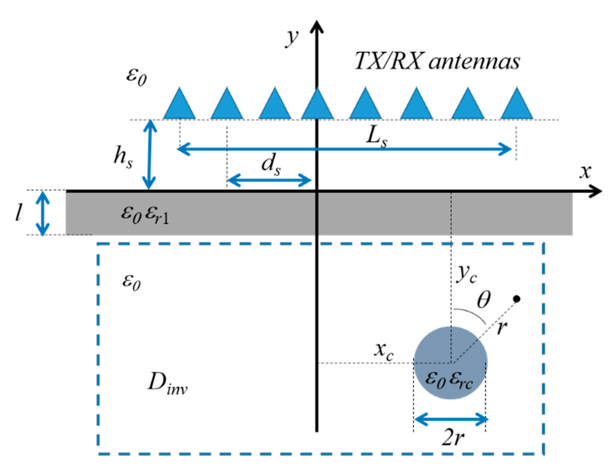
Abstract
1. Introduction
2. Theoretical Approach to the Through-Wall Imaging Problem
2.1. Forward-Scattering Problem Formulation
2.2. Inverse-Scattering Problem Formulation
- Set the outer iteration index to and initialize the contrast function at the first outer step with .
- Linearize the scattering problem by computing the Fréchet derivative of the operator around the current solution . A linear problem is then obtained. It is worth remarking that, similarly to the corresponding procedures in free space [31,33], the computation of the right-hand side of the linear problem and of the Fréchet derivative requires the solution of a set of forward problems. To this end, a forward solver based on the MoM is adopted.
- Solve the obtained linear problem in a regularized sense by means of the Lebesgue-space procedure detailed in [31,33]. Specifically, the solution of the linear problem obtained in step 2, i.e., , is computed by means of the following Landweber-type iterations:where is a relaxation coefficient, is the Hölder conjugate of , and the duality map is defined as , with = (if , otherwise it is equal to zero).
- Update the contrast function by adding the solution of the linear problem found at step 3 to the current value, i.e.,
- Iterate from step 2 until a proper stopping criterion is satisfied.
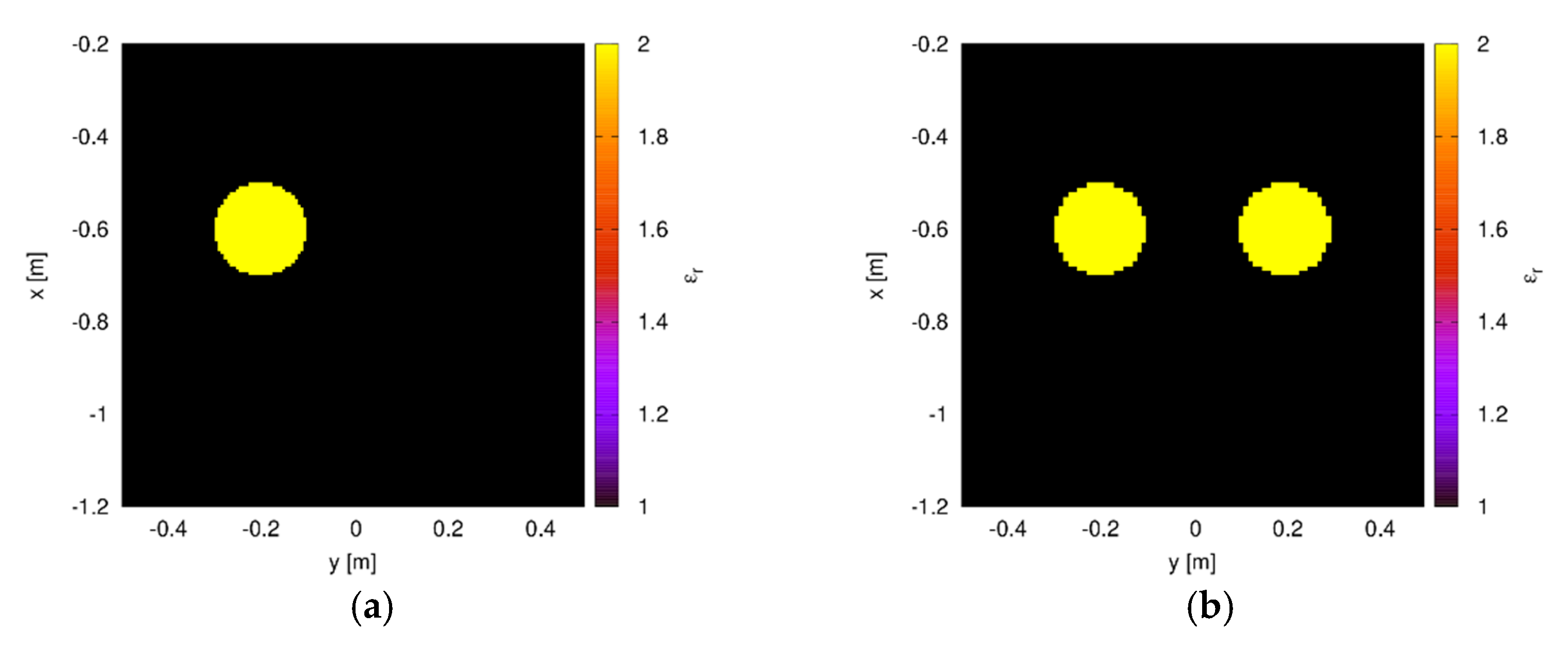
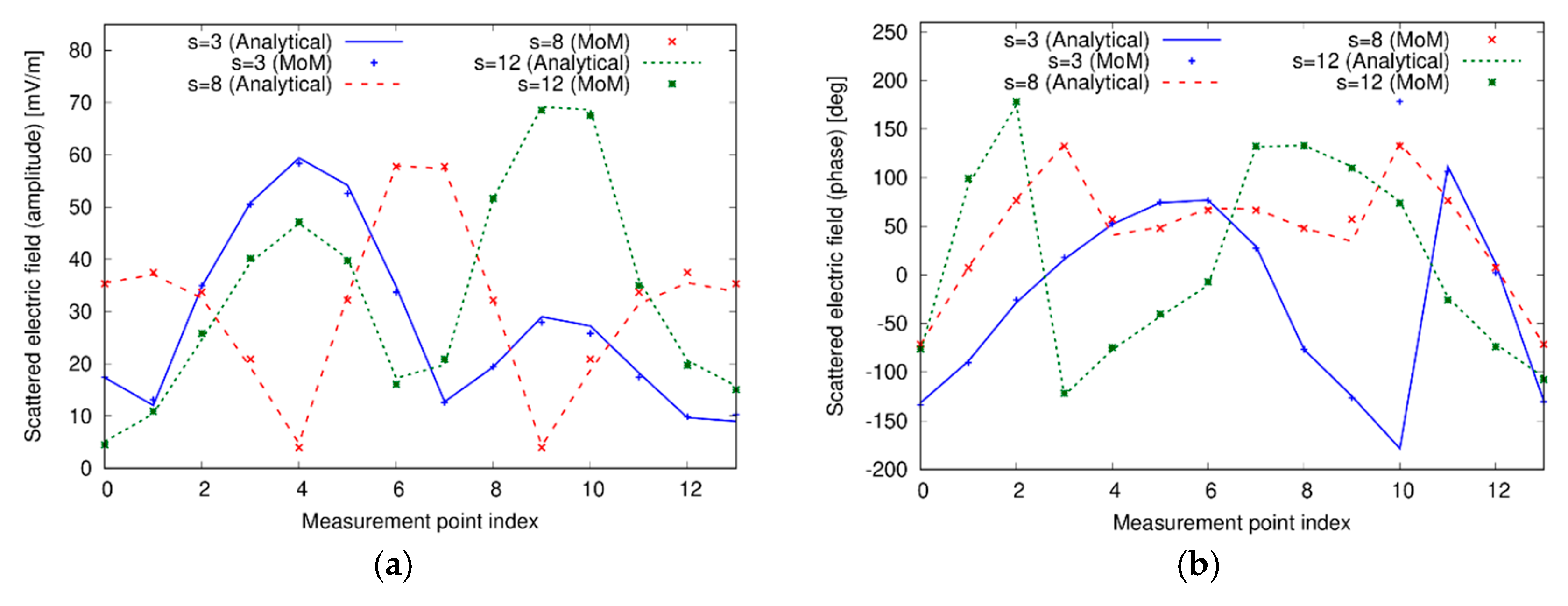
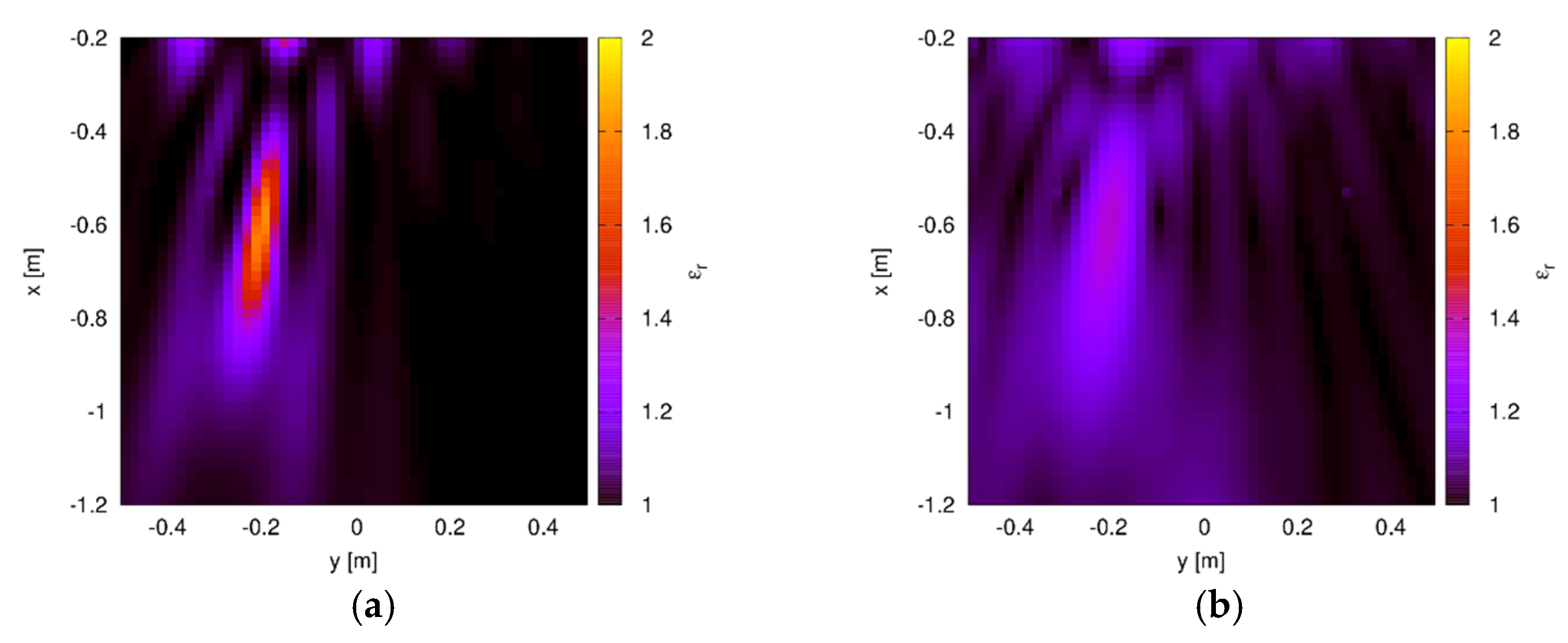
3. Numerical Results
3.1. Validation of the Forward Methods
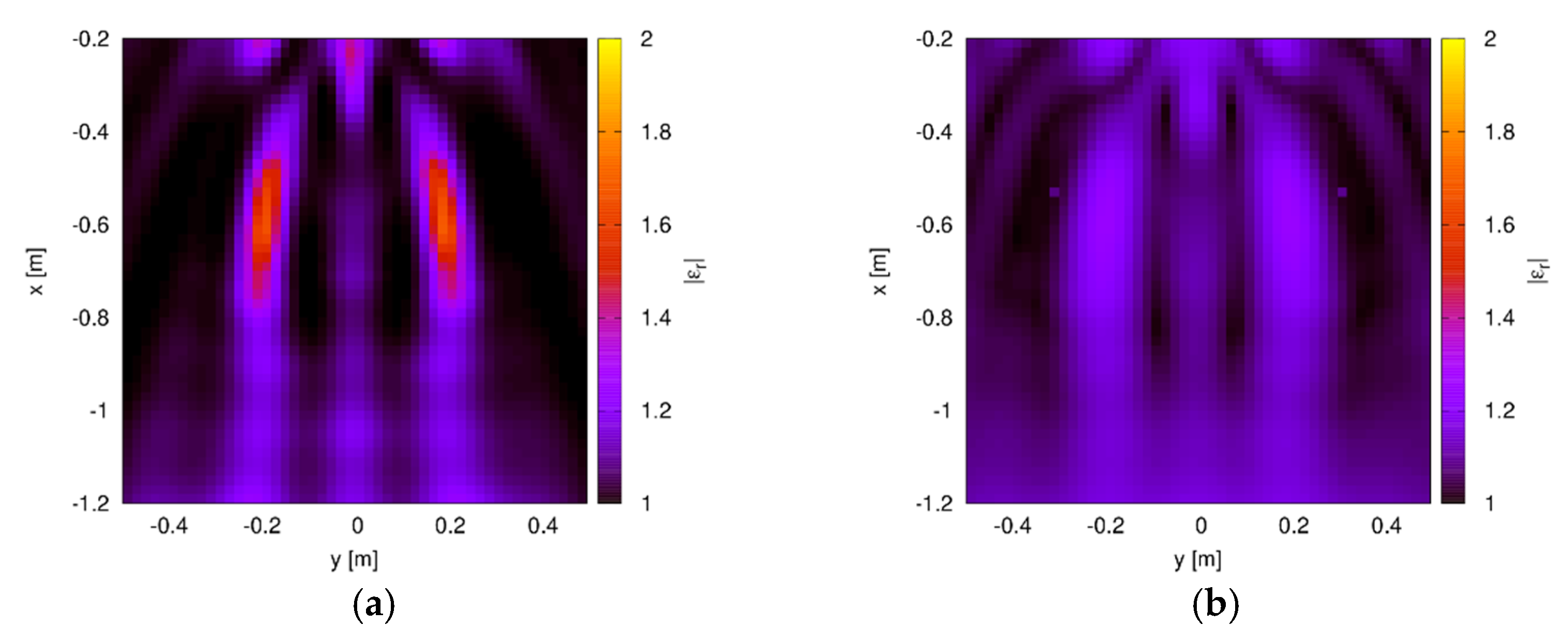
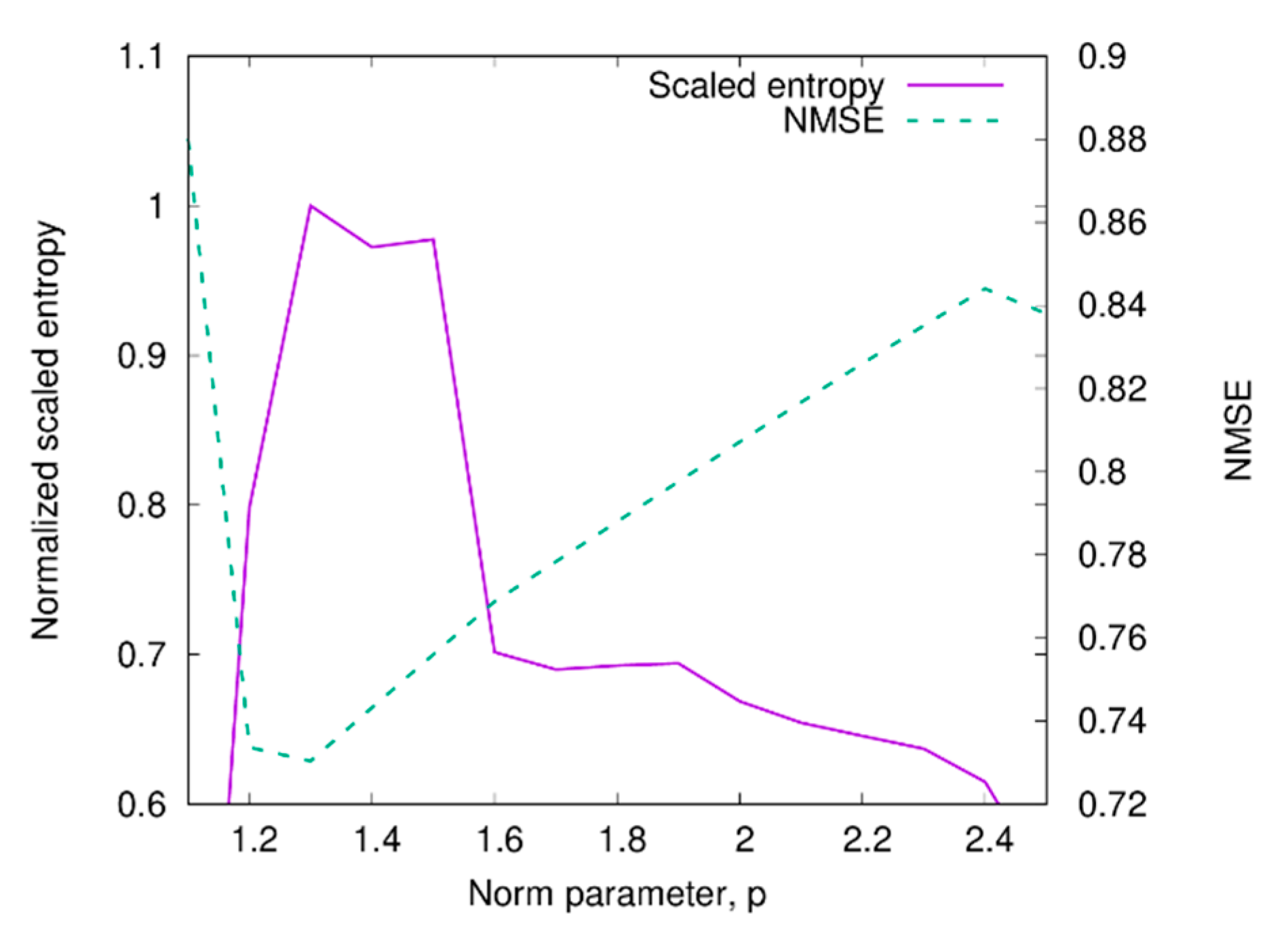
3.2. Inversion Scheme
4. Conclusions
Author Contributions
Funding
Conflicts of Interest
References
- Amin, M.G. Through-The-Wall Radar Imaging; CRC Press: Boca Raton, FL, USA, 2011; ISBN 978-1-4398-1476-5. [Google Scholar]
- Soldovieri, F.; Solimene, R. Through-Wall imaging via a linear inverse scattering algorithm. IEEE Geosci. Remote Sens. Lett. 2007, 4, 513–517. [Google Scholar] [CrossRef]
- Gennarelli, G.; Vivone, G.; Braca, P.; Soldovieri, F.; Amin, M.G. Multiple extended target tracking for through-wall radars. IEEE Trans. Geosci. Remote Sens. 2015, 53, 6482–6494. [Google Scholar] [CrossRef]
- Yektakhah, B.; Sarabandi, K. All-directions through-the-wall radar imaging using a small number of moving transceivers. IEEE Trans. Geosci. Remote Sens. 2016, 54, 6415–6428. [Google Scholar] [CrossRef]
- Yektakhah, B.; Sarabandi, K. All-Directions Through-the-Wall Imaging Using a Small Number of Moving Omnidirectional Bi-Static FMCW Transceivers. IEEE Trans. Geosci. Remote Sens. 2019, 57, 2618–2627. [Google Scholar] [CrossRef]
- Boudamouz, B.; Millot, P.; Pichot, C. Through the Wall Radar Imaging with MIMO beamforming processing - Simulation and Experimental Results. Am. J. Remote Sens. 2013, 1, 7–12. [Google Scholar] [CrossRef][Green Version]
- Chew, W.C. Waves and Fields in Inhomogeneous Media; IEEE Press Series on Electromagnetic Wawes; IEEE Press: Piscataway, NY, USA, 1995; ISBN 978-0-7803-4749-6. [Google Scholar]
- Dehmollaian, M.; Sarabandi, K. Hybrid Fdtd and Ray Optics Approximation for Simulation of Through-Wall Microwave Imaging. In Proceedings of the IEEE Antennas and Propagation Society International Symposium, Albuquerque, NM, USA, 9–14 July 2006; pp. 249–252. [Google Scholar]
- Warren, C.; Giannopoulos, A.; Giannakis, I. gprMax: Open source software to simulate electromagnetic wave propagation for Ground Penetrating Radar. Comput. Phys. Commun. 2016, 209, 163–170. [Google Scholar] [CrossRef]
- Chang, P.C.; Burkholder, R.J.; Volakis, J.L.; Marhefka, R.J.; Bayram, Y. High-Frequency EM Characterization of Through-Wall Building Imaging. IEEE Trans. Geosci. Remote Sens. 2009, 47, 1375–1387. [Google Scholar] [CrossRef]
- Antonopoulos, C.S.; Kantartzis, N.V.; Rekanos, I.T. FDTD Method for Wave Propagation in Havriliak-Negami Media Based on Fractional Derivative Approximation. IEEE Trans. Magn. 2017, 53. [Google Scholar] [CrossRef]
- Guo, Q.; Li, Y.; Liang, X.; Dong, J.; Cheng, R. Through-the-Wall Image Reconstruction via Reweighted Total Variation and Prior Information in Radio Tomographic Imaging. IEEE Access 2020, 8, 40057–40066. [Google Scholar] [CrossRef]
- Doğu, S.; Akıncı, M.N.; Çayören, M.; Akduman, İ. Truncated Singular Value Decomposition for Through-the-Wall Microwave Imaging Application. IET Microw. Antennas Propag. 2020, 14, 260–267. [Google Scholar] [CrossRef]
- Charnley, M.; Wood, A. A Linear Sampling Method for Through-the-Wall Radar Detection. J. Comput. Phys. 2017, 347, 147–159. [Google Scholar] [CrossRef]
- Aamna, M.; Ammar, S.; Rameez, T.; Shabeeb, S.; Naveed, I.R.; Safwat, I. 2D Beamforming for Through-the-Wall Microwave Imaging applications. In Proceedings of the 2010 International Conference on Information and Emerging Technologies, Karachi, Pakistan, 14–16 June 2010; pp. 1–6. [Google Scholar]
- Mizrahi, M.; Holdengreber, E.; Schacham, S.E.; Farber, E.; Zalevsky, Z. Improving Radar’s Spatial Recognition: A Radar Scanning Method Based on Microwave Spatial Spectral Illumination. IEEE Microw. Mag. 2016, 17, 28–34. [Google Scholar] [CrossRef]
- Mizrahi, M.; Holdengreber, E.; Farber, E.; Zalevsky, Z. Frequency Multiplexing Spatial Super-Resolved Sensing for RADAR Applications. Microw. Opt. Technol. Lett. 2016, 58, 831–835. [Google Scholar] [CrossRef]
- Zhao, M.; Li, T.; Alsheikh, M.A.; Tian, Y.; Zhao, H.; Torralba, A.; Katabi, D. Through-Wall Human Pose Estimation Using Radio Signals. In Proceedings of the 2018 IEEE/CVF Conference on Computer Vision and Pattern Recognition, Salt Lake City, UT, USA, 18–22 June 2018; pp. 7356–7365. [Google Scholar]
- Keith, S.R. Discrimination Between Child and Adult Forms Using Radar Frequency Signature Analysis; AFIT-ENP-13-M-20; Air Force Institute of Technology: Wright-Patterson Air Force Base, OH, USA, 2013. [Google Scholar]
- Nikolova, N.D. Introduction to Microwave Imaging; Cambridge University Press: Cambridge, UK, 2017; ISBN 978-1-316-08426-7. [Google Scholar]
- Pastorino, M.; Randazzo, A. Microwave Imaging Methods and Applications; Artech House: Boston, MA, USA, 2018; ISBN 978-1-63081-348-2. [Google Scholar]
- Crocco, L.; Catapano, I.; Di Donato, L.; Isernia, T. The linear sampling method as a way to quantitative inverse scattering. IEEE Trans. Antennas Propag. 2012, 60, 1844–1853. [Google Scholar] [CrossRef]
- Bozza, G.; Pastorino, M. An inexact Newton-based approach to microwave imaging within the contrast source formulation. IEEE Trans. Antennas Propag. 2009, 57, 1122–1132. [Google Scholar] [CrossRef]
- De Zaeytijd, J.; Franchois, A.; Eyraud, C.; Geffrin, J.-M. Full-wave three-dimensional microwave imaging with a regularized Gauss-Newton method - Theory and experiment. IEEE Trans. Antennas Propag. 2007, 55, 3279–3292. [Google Scholar] [CrossRef]
- Oliveri, G.; Lizzi, L.; Pastorino, M.; Massa, A. A nested multi-scaling inexact-Newton iterative approach for microwave imaging. IEEE Trans. Antennas Propag. 2012, 60, 971–983. [Google Scholar] [CrossRef]
- Li, M.; Semerci, O.; Abubakar, A. A contrast source inversion method in the wavelet domain. Inverse Probl. 2013, 29, 025015. [Google Scholar] [CrossRef]
- Semnani, A.; Rekanos, I.T.; Kamyab, M.; Moghaddam, M. Solving Inverse Scattering Problems Based on Truncated Cosine Fourier and Cubic B-Spline Expansions. IEEE Trans. Antennas Propag. 2012, 60, 5914–5923. [Google Scholar] [CrossRef]
- Monleone, R.D.; Pastorino, M.; Fortuny-Guasch, J.; Salvade, A.; Bartesaghi, T.; Bozza, G.; Maffongelli, M.; Massimini, A.; Carbonetti, A.; Randazzo, A. Impact of background noise on dielectric reconstructions obtained by a prototype of microwave axial tomograph. IEEE Trans. Instrum. Meas. 2012, 61, 140–148. [Google Scholar] [CrossRef]
- Zeitler, A.; Migliaccio, C.; Moynot, A.; Aliferis, I.; Brochier, L.; Dauvignac, J.-Y.; Pichot, C. Amplitude and phase measurements of scattered fields for quantitative imaging in the W-band. IEEE Trans. Antennas Propag. 2013, 61, 3927–3931. [Google Scholar] [CrossRef]
- Ye, X.; Chen, X. Subspace-Based Distorted-Born Iterative Method for Solving Inverse Scattering Problems. IEEE Trans. Antennas Propag. 2017, 65, 7224–7232. [Google Scholar] [CrossRef]
- Estatico, C.; Pastorino, M.; Randazzo, A. A novel microwave imaging approach based on regularization in Lp Banach spaces. IEEE Trans. Antennas Propag. 2012, 60, 3373–3381. [Google Scholar] [CrossRef]
- Estatico, C.; Fedeli, A.; Pastorino, M.; Randazzo, A. Microwave imaging of elliptically shaped dielectric cylinders by means of an Lp Banach-space inversion algorithm. Meas. Sci. Technol. 2013, 24, 074017. [Google Scholar] [CrossRef]
- Estatico, C.; Pastorino, M.; Randazzo, A.; Tavanti, E. Three-dimensional microwave imaging in Lp Banach spaces: Numerical and experimental results. IEEE Trans. Comput. Imaging 2018, 4, 609–623. [Google Scholar] [CrossRef]
- Estatico, C.; Fedeli, A.; Pastorino, M.; Randazzo, A. Quantitative microwave imaging method in Lebesgue spaces with nonconstant exponents. IEEE Trans. Antennas Propag. 2018, 66, 7282–7294. [Google Scholar] [CrossRef]
- Estatico, C.; Fedeli, A.; Pastorino, M.; Randazzo, A. Microwave imaging by means of Lebesgue-space inversion: An overview. Electronics 2019, 8, 945. [Google Scholar] [CrossRef]
- Estatico, C.; Fedeli, A.; Pastorino, M.; Randazzo, A. A multifrequency inexact-Newton method in Lp Banach spaces for buried objects detection. IEEE Trans. Antennas Propag. 2015, 63, 4198–4204. [Google Scholar] [CrossRef]
- Ponti, C.; Santarsiero, M.; Schettini, G. Electromagnetic scattering of a pulsed signal by conducting cylindrical targets embedded in a half-space medium. IEEE Trans. Antennas Propag. 2017, 65, 3073–3083. [Google Scholar] [CrossRef]
- Frezza, F.; Pajewski, L.; Ponti, C.; Schettini, G. Through-wall electromagnetic scattering by N conducting cylinders. J. Opt. Soc. Am. A Opt. Image Sci. Vis. 2013, 30, 1632–1639. [Google Scholar] [CrossRef]
- Ponti, C.; Vellucci, S. Scattering by conducting cylinders below a dielectric layer with a fast noniterative approach. IEEE Trans. Microw. Theory Tech. 2015, 63, 30–39. [Google Scholar] [CrossRef]
- Ponti, C.; Schettini, G. Direct scattering methods in presence of interfaces with different media. In Proceedings of the 11th European Conference on Antennas and Propagation, Paris, France, 19–24 March 2017; pp. 1707–1710. [Google Scholar]
- Ponti, C.; Schettini, G. The cylindrical wave approach for the electromagnetic scattering by targets behind a wall. Electronics 2019, 8, 1262. [Google Scholar] [CrossRef]
- Balanis, C.A. Advanced Engineering Electromagnetics, 2nd ed.; John Wiley & Sons: Hoboken, NJ, USA, 2012; ISBN 978-0-470-58948-9. [Google Scholar]
- Orfanidis, S.J. Electromagnetic Waves and Antennas. 2016. Available online: http://www.ece.rutgers.edu/~orfanidi/ewa/ (accessed on 18 May 2020).
- Wei, X.; Zhang, Y. Autofocusing Techniques for GPR Data from RC Bridge Decks. IEEE J. Sel. Top. Appl. Earth Obs. Remote Sens. 2014, 7, 4860–4868. [Google Scholar] [CrossRef]
- Giannakis, I.; Tosti, F.; Lantini, L.; Alani, A.M. Diagnosing Emerging Infectious Diseases of Trees Using Ground Penetrating Radar. IEEE Trans. Geosci. Remote Sens. 2020, 58, 1146–1155. [Google Scholar] [CrossRef]


© 2020 by the authors. Licensee MDPI, Basel, Switzerland. This article is an open access article distributed under the terms and conditions of the Creative Commons Attribution (CC BY) license (http://creativecommons.org/licenses/by/4.0/).
Share and Cite
Fedeli, A.; Pastorino, M.; Ponti, C.; Randazzo, A.; Schettini, G. Through-the-Wall Microwave Imaging: Forward and Inverse Scattering Modeling. Sensors 2020, 20, 2865. https://doi.org/10.3390/s20102865
Fedeli A, Pastorino M, Ponti C, Randazzo A, Schettini G. Through-the-Wall Microwave Imaging: Forward and Inverse Scattering Modeling. Sensors. 2020; 20(10):2865. https://doi.org/10.3390/s20102865
Chicago/Turabian StyleFedeli, Alessandro, Matteo Pastorino, Cristina Ponti, Andrea Randazzo, and Giuseppe Schettini. 2020. "Through-the-Wall Microwave Imaging: Forward and Inverse Scattering Modeling" Sensors 20, no. 10: 2865. https://doi.org/10.3390/s20102865
APA StyleFedeli, A., Pastorino, M., Ponti, C., Randazzo, A., & Schettini, G. (2020). Through-the-Wall Microwave Imaging: Forward and Inverse Scattering Modeling. Sensors, 20(10), 2865. https://doi.org/10.3390/s20102865