A Prototype Microwave System for 3D Brain Stroke Imaging

 ,
,  ,
,  ,
,  , , ,
, , ,  , and
, and 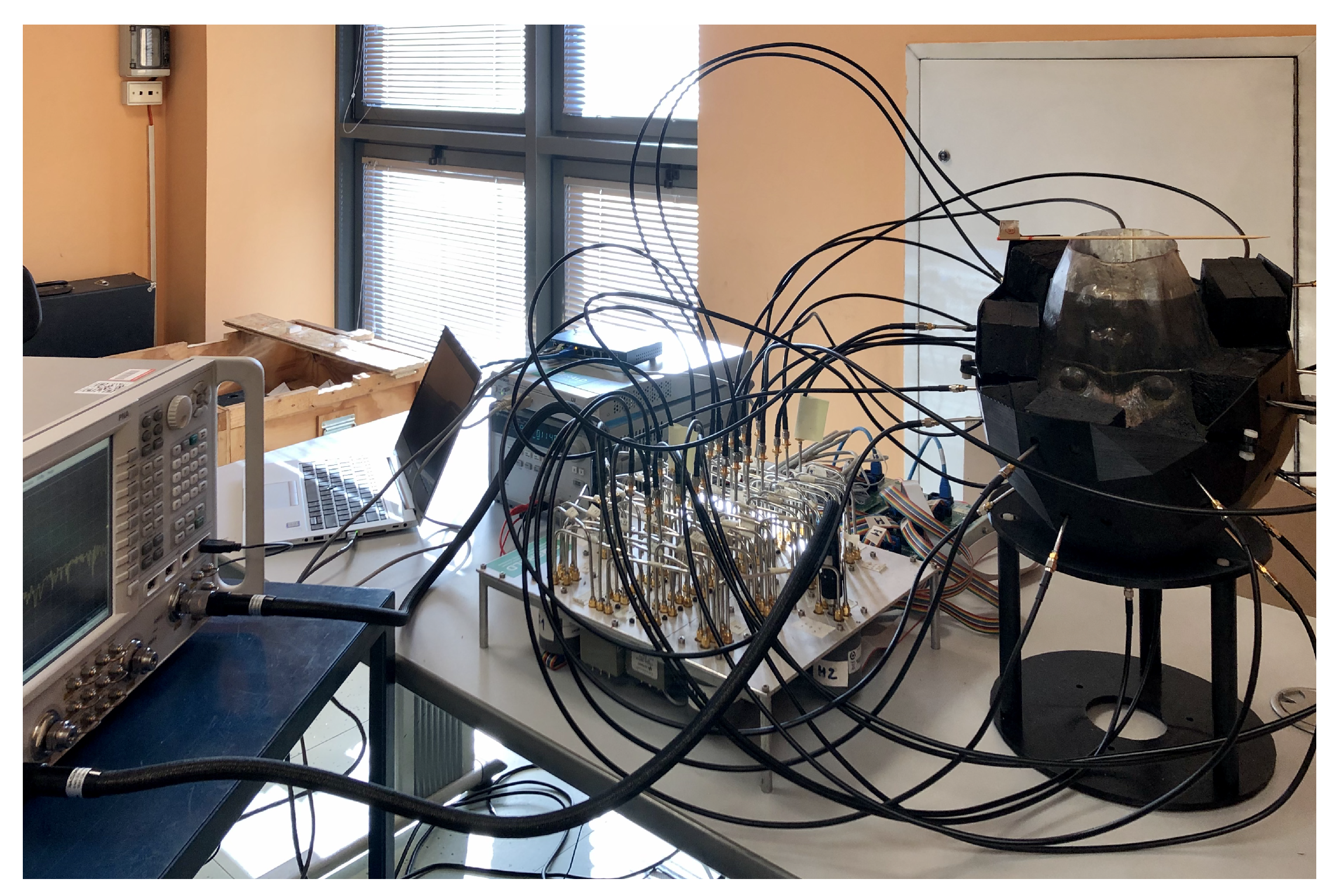
Abstract
1. Introduction
2. Material and Methods
2.1. Three-Dimensional Microwave Imaging System Design
2.2. Three-Dimensional Microwave Imaging System Realization
2.2.1. Vector Network Analyzer and Switching Matrix
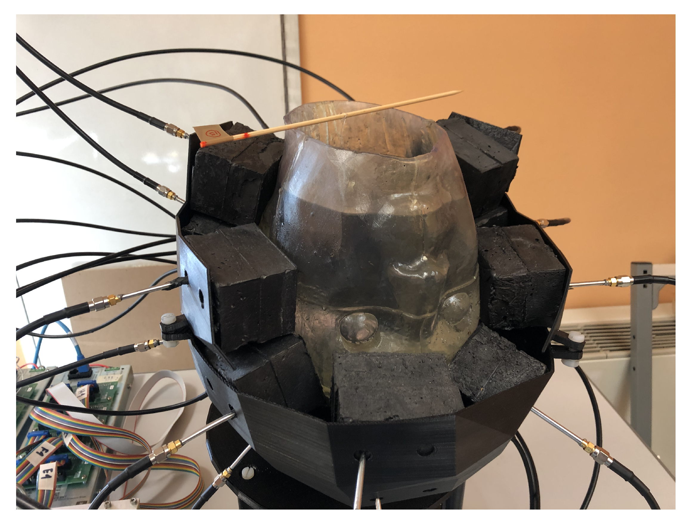
2.2.2. Brick Antenna Array
2.2.3. Anthropomorphic Head Phantom
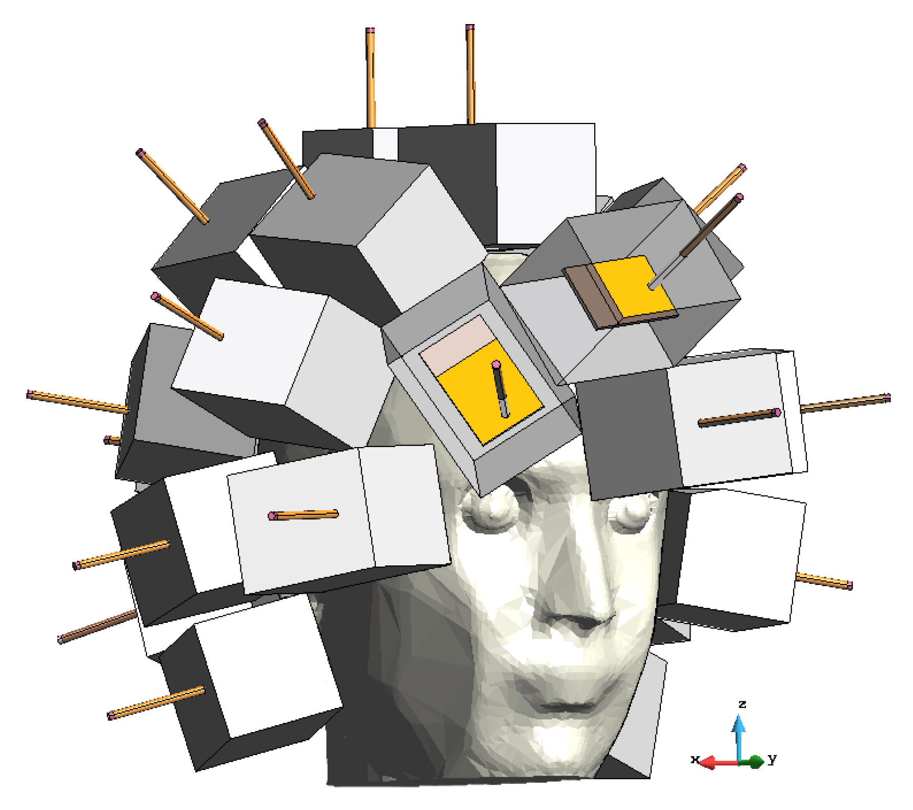
2.2.4. Digital Twin of the Device
2.2.5. Experiment Set-Up
3. Results
3.1. Numerical Assessment
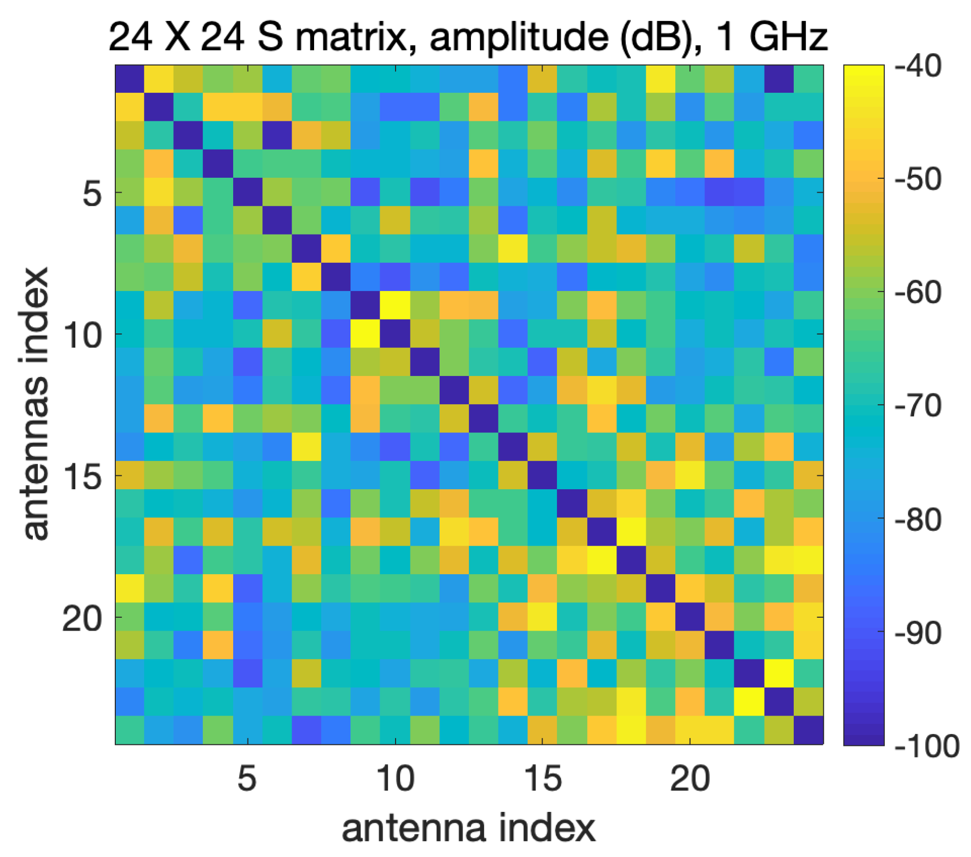
3.2. Experimental Validation
4. Discussion
5. Conclusions and Future Work
Author Contributions
Funding
Acknowledgments
Conflicts of Interest
Abbreviations
| MRI | Magnetic resonance imaging |
| CT | Computerized tomography |
| MWI | Microwave imaging |
| VNA | Vector network analyzer |
| EM | Electromagnetic |
| SNR | Signal-to-noise ratio |
| TSVD | Truncated singular value decomposition |
| SP4T | Single-pole-four-throw |
| SPDT | Single-pole-double-throw |
| IF | Intermediate frequency |
| TX | Transmitter |
| RX | Receiver |
| ABS | Acrylonitrile butadiene styrene |
| STL | Stereo-lithography |
| FEM | Finite element method |
| PEC | Perfect electric conductor |
| ABC | Absorbing boundary conditions |
| CAD | Proper computer-aided design |
| RMSE | Root mean square error |
References
- Benjamin, E.J.; Muntner, P.; Bittencourt, M.S. Heart Disease and Stroke Statistics—2019 Update: A Report from the American Heart Association. Circulation 2019, 139, e56–e528. [Google Scholar] [CrossRef] [PubMed]
- Eurostat. Healthcare Resource Statistics—Technical Resources and Medical Technology; Eurostat: Luxembourg, 2019. [Google Scholar]
- Walsh, K.B. Non-invasive Sensor Technology for Prehospital Stroke Diagnosis: Current Status and Future Directions. Int. J. Stroke 2019, 14, 592–602. [Google Scholar] [CrossRef] [PubMed]
- Crocco, L.; Karanasiou, I.; James, M.; Conceicao, R.C. Emerging Electromagnetic Technologies for Brain Diseases Diagnostics, Monitoring and Therapy; Crocco, L., Karanasiou, I., James, M., Eds.; Springer International Publishing: Cham, Switzerland, 2018. [Google Scholar]
- Casu, M.R.; Vacca, M.; Tobon Vasquez, J.A.; Pulimeno, A.; Sarwar, I.; Solimene, R.; Vipiana, F. A COTS-Based Microwave Imaging System for Breast-Cancer Detection. IEEE Trans. Biomed. Circuits Syst. 2017, 11, 804–814. [Google Scholar] [CrossRef] [PubMed]
- Sarwar, I.; Turvani, G.; Casu, M.R.; Tobon Vasquez, J.A.; Vipiana, F.; Scapaticci, R.; Crocco, L. Low-Cost Low-Power Acceleration of a Microwave Imaging Algorithm for Brain Stroke Monitoring. J. Low Power Electron. Appl. 2018, 8, 43. [Google Scholar] [CrossRef]
- Persson, M.; Fhager, A.; Trefnà, H.D.; Yu, Y.; McKelvey, T.; Pegenius, G.; Karlsson, J.E.; Elam, M. Microwave-Based Stroke Diagnosis Making Global Prehospital Thrombolytic Treatment Possible. IEEE Trans. Biomed. Eng. 2014, 61, 2806–2817. [Google Scholar] [CrossRef]
- Candefjord, S.; Winges, J.; Malik, A.; Yu, Y.; Rylander, T.; McKelvey, T.; Fhager, A.; Elam, M.; Persson, M. Microwave Technology for Detecting Traumatic Intracranial Bleedings: Tests on Phantom of Subdural Hematoma and Numerical Simulations. Med. Biol. Eng. Comput. 2017, 55, 1177–1188. [Google Scholar] [CrossRef]
- Fhager, A.; Candefjord, S.; Elam, M.; Persson, M. Microwave Diagnostics Ahead: Saving Time and the Lives of Trauma and Stroke Patients. IEEE Microw. Mag. 2018, 19, 78–90. [Google Scholar] [CrossRef]
- Hopfer, M.; Planas, R.; Hamidipour, A.; Henriksson, T.; Semenov, S. Electromagnetic Tomography for Detection, Differentiation, and Monitoring of Brain Stroke: A Virtual Data and Human Head Phantom Study. IEEE Antennas Propag. Mag. 2017, 59, 86–97. [Google Scholar] [CrossRef]
- Afsari, A.; Abbosh, A.M.; Rahmat-Samii, Y. Modified Born Iterative Method in Medical Electromagnetic Tomography Using Magnetic Field Fluctuation Contrast Source Operator. IEEE Trans. Microw. Theory Tech. 2019, 67, 454–463. [Google Scholar] [CrossRef]
- Mobashsher, A.T.; Abbosh, A.M. On-site Rapid Diagnosis of Intracranial Hematoma using Portable Multi-slice Microwave Imaging System. Sci. Rep. 2016, 6, 37620. [Google Scholar] [CrossRef]
- Alqadami, A.S.M.; Bialkowski, K.S.; Mobashsher, A.T.; Abbosh, A.M. Wearable Electromagnetic Head Imaging System Using Flexible Wideband Antenna Array Based on Polymer Technology for Brain Stroke Diagnosis. IEEE Trans. Biomed. Circuits Syst. 2019, 13, 124–134. [Google Scholar] [CrossRef] [PubMed]
- Maffongelli, M.; Poretti, S.; Salvade, A.; Monleone, R.; Pagnamenta, C.; Fedeli, A.; Pastorino, M.; Randazzo, A. Design and Experimental Test of a Microwave System for Quantitative Biomedical Imaging. In Proceedings of the IEEE International Symposium on Medical Measurements and Applications (MeMeA), Rome, Italy, 11–13 June 2018. [Google Scholar]
- Merunka, I.; Massa, A.; Vrba, D.; Fiser, O.; Salucci, M.; Vrba, J. Microwave Tomography System for Methodical Testing of Human Brain Stroke Detection Approaches. Int. J. Antennas Propag. 2019, 2019, 9. [Google Scholar] [CrossRef]
- Karadima, O.; Rahman, M.; Sotiriou, I.; Ghavami, N.; Lu, P.; Ahsan, S.; Kosmas, P. Experimental Validation of Microwave Tomography with the DBIM-TwIST Algorithm for Brain Stroke Detection and Classification. Sensors 2020, 20, 840. [Google Scholar] [CrossRef] [PubMed]
- Bisio, I.; Fedeli, A.; Lavagetto, F.; Pastorino, M.; Sciarrone, A.R.A.; Tavanti, E. A Numerical Study Concerning Brain Stroke Detection by Microwave Imaging Systems. Multimed. Tools Appl. 2017, 77, 9341–9363. [Google Scholar] [CrossRef]
- Scapaticci, R.; Tobon Vasquez, J.A.; Bellizzi, G.; Vipiana, F.; Crocco, L. Design and Numerical Characterization of a Low-Complexity Microwave Device for Brain Stroke Monitoring. IEEE Trans. Antennas Propag. 2018, 66, 7328–7338. [Google Scholar] [CrossRef]
- Scapaticci, R.; Bucci, O.; Catapano, I.; Crocco, L. Differential Microwave Imaging for Brain Stroke Follow up. Int. J. Antennas Propag. 2014, 2014, 11. [Google Scholar] [CrossRef]
- Scapaticci, R.; Donato, L.D.; Catapano, I.; Crocco, L. A feasibility study on Microwave Imaging for Brain Stroke Monitoring. Prog. Electromagn. Res. B 2012, 40, 305–324. [Google Scholar] [CrossRef]
- Bucci, O.M.; Crocco, L.; Scapaticci, R.; Bellizzi, G. On the Design of Phased Arrays for Medical Applications. Proc. IEEE 2016, 104, 633–648. [Google Scholar] [CrossRef]
- Bertero, M.; Boccacci, P. Introduction to Inverse Problems in Imaging; CRC Press: Boca Raton, FL, USA, 1998. [Google Scholar]
- Tobon Vasquez, J.A.; Scapaticci, R.; Turvani, G.; Bellizzi, G.; Joachimowicz, N.; Duchêne, B.; Tedeschi, E.; Casu, M.R.; Crocco, L.; Vipiana, F. Design and Experimental Assessment of a 2D Microwave Imaging System for Brain Stroke Monitoring. Int. J. Antennas Propag. 2019, 2019, 12. [Google Scholar] [CrossRef]
- Meaney, P.M.; Shubitidze, F.; Fanning, M.W.; Kmiec, M.; Epstein, N.R.; Paulsen, K.D. Surface Wave Multipath Signals in Near-Field Microwave Imaging. Int. J. Biomed. Imag. 2012, 2012, 11. [Google Scholar] [CrossRef]
- Keysight Technologies. Keysight Technologies. Keysight 2-Port and 4-Port PNA Network Analyzer, N5227A 10 MHz to 67 GHz. In Data Sheet and Technical Specifications; Keysight Technologies: Santa Rosa, CA, USA, 2019. [Google Scholar]
- Graedel, N.N.; Polimeni, J.R.; Guerin, B.; Gagoski, B.; Wald, L.L. An Anatomically Realistic Temperature Phantom for Radio Frequency Heating Measurements. Magn. Reson. Med. 2015, 73, 442–450. [Google Scholar] [CrossRef] [PubMed]
- Joachimowicz, N.; Duchêne, B.; Conessa, C.; Meyer, O. Anthropomorphic Breast and Head Phantoms for Microwave Imaging. Diagnostics 2018, 8, 85. [Google Scholar] [CrossRef] [PubMed]
- Attardo, E.A.; Borsic, A.; Vecchi, G.; Meaney, P.M. Whole-System Electromagnetic Modeling for Microwave Tomography. IEEE Antennas Wirel. Propag. Lett. 2012, 11, 1618–1621. [Google Scholar] [CrossRef]
- Abedi, S.; Joachimowicz, N.; Duchêne, B.; Roussel, H.; Tobon Vasquez, J.A.; Rodriguez-Duarte, D.; Scapaticci, R.; Crocco, L.; Vipiana, F. Benchmark Head Phantoms for Microwave Imaging of Brain Strokes. In Proceedings of the 42nd Photonics & Electromagnetics Research Symposium (PIERS), Xiamen, China, 17–20 December 2019. [Google Scholar]


© 2020 by the authors. Licensee MDPI, Basel, Switzerland. This article is an open access article distributed under the terms and conditions of the Creative Commons Attribution (CC BY) license (http://creativecommons.org/licenses/by/4.0/).
Share and Cite
Tobon Vasquez, J.A.; Scapaticci, R.; Turvani, G.; Bellizzi, G.; Rodriguez-Duarte, D.O.; Joachimowicz, N.; Duchêne, B.; Tedeschi, E.; Casu, M.R.; Crocco, L.; et al. A Prototype Microwave System for 3D Brain Stroke Imaging. Sensors 2020, 20, 2607. https://doi.org/10.3390/s20092607
Tobon Vasquez JA, Scapaticci R, Turvani G, Bellizzi G, Rodriguez-Duarte DO, Joachimowicz N, Duchêne B, Tedeschi E, Casu MR, Crocco L, et al. A Prototype Microwave System for 3D Brain Stroke Imaging. Sensors. 2020; 20(9):2607. https://doi.org/10.3390/s20092607
Chicago/Turabian StyleTobon Vasquez, Jorge A., Rosa Scapaticci, Giovanna Turvani, Gennaro Bellizzi, David O. Rodriguez-Duarte, Nadine Joachimowicz, Bernard Duchêne, Enrico Tedeschi, Mario R. Casu, Lorenzo Crocco, and et al. 2020. "A Prototype Microwave System for 3D Brain Stroke Imaging" Sensors 20, no. 9: 2607. https://doi.org/10.3390/s20092607
APA StyleTobon Vasquez, J. A., Scapaticci, R., Turvani, G., Bellizzi, G., Rodriguez-Duarte, D. O., Joachimowicz, N., Duchêne, B., Tedeschi, E., Casu, M. R., Crocco, L., & Vipiana, F. (2020). A Prototype Microwave System for 3D Brain Stroke Imaging. Sensors, 20(9), 2607. https://doi.org/10.3390/s20092607