Performance Analysis of Ionospheric Scintillation Effect on P-Band Sliding Spotlight SAR System


Abstract
:1. Introduction
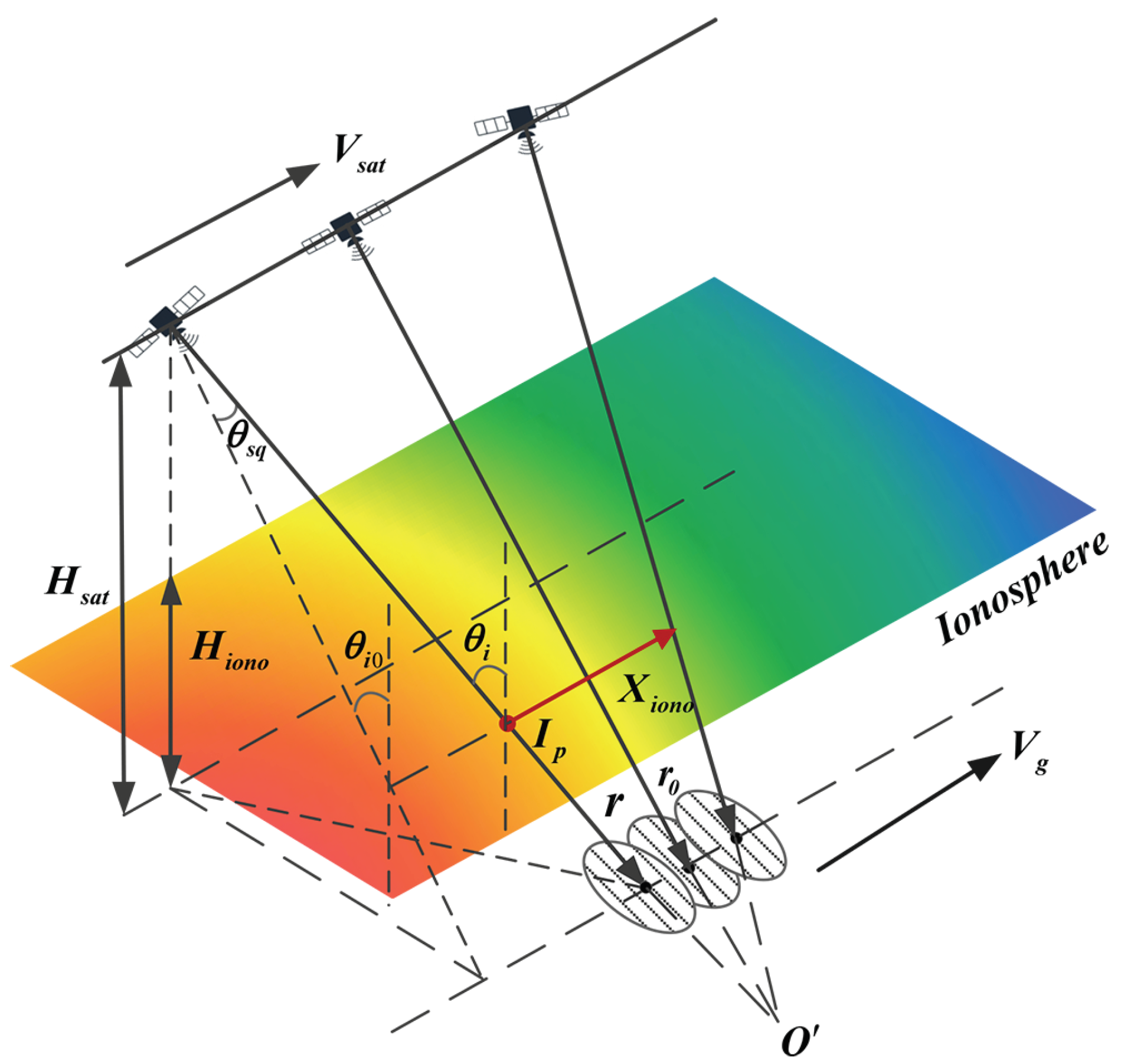
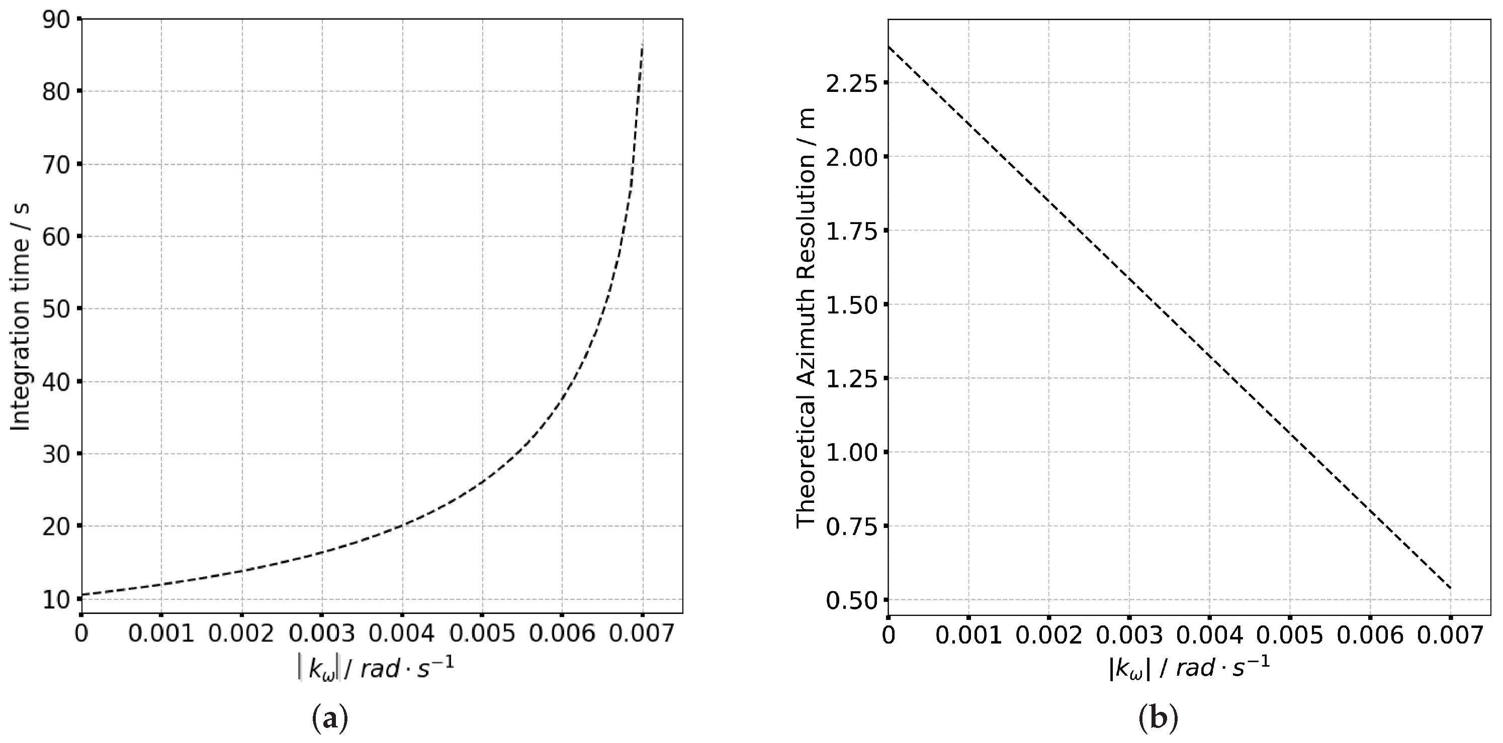
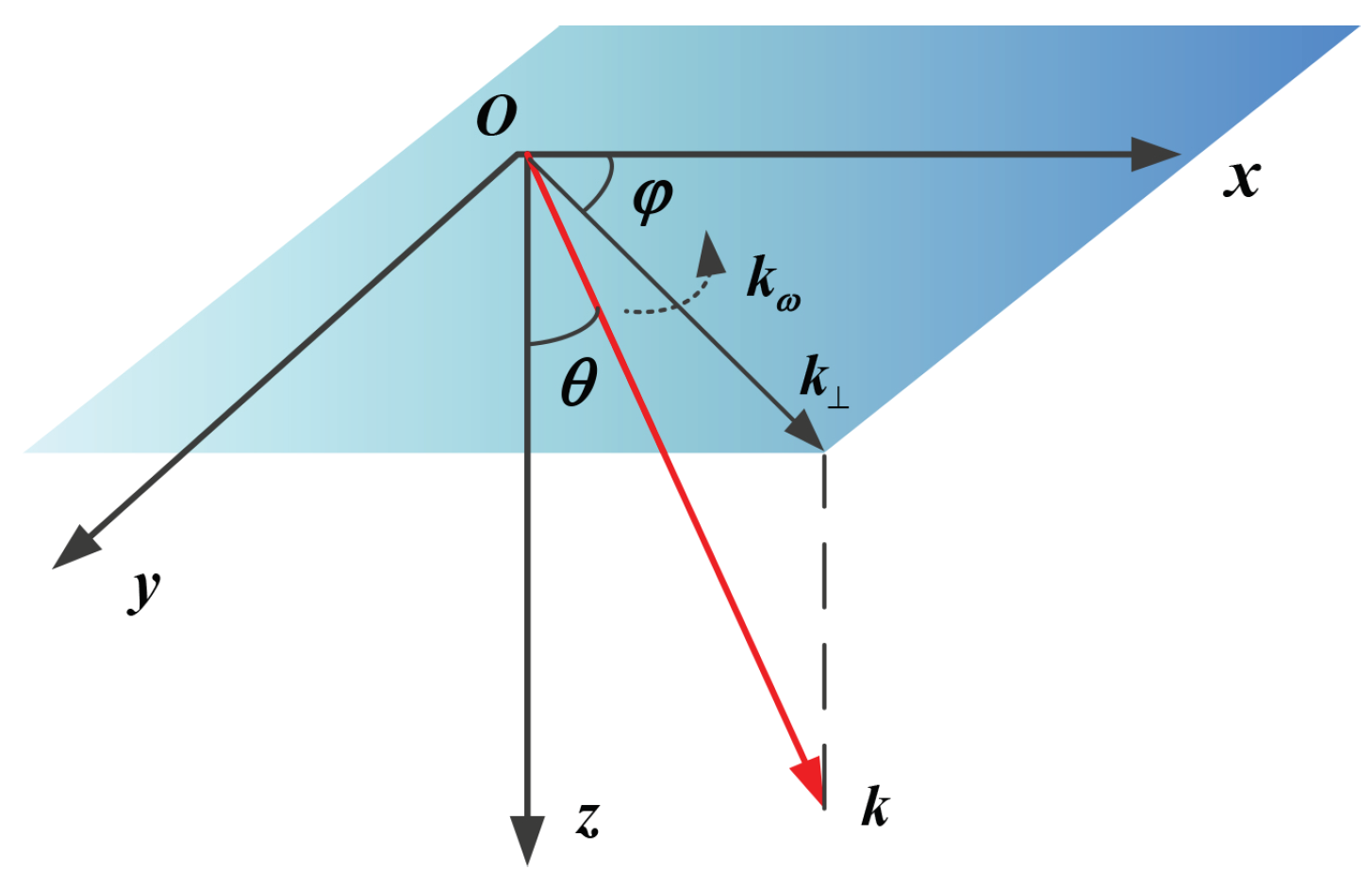
2. The Observation Geometry of Sliding Spotlight SAR System
3. Theoretical Analysis Based on TFTPCF Model
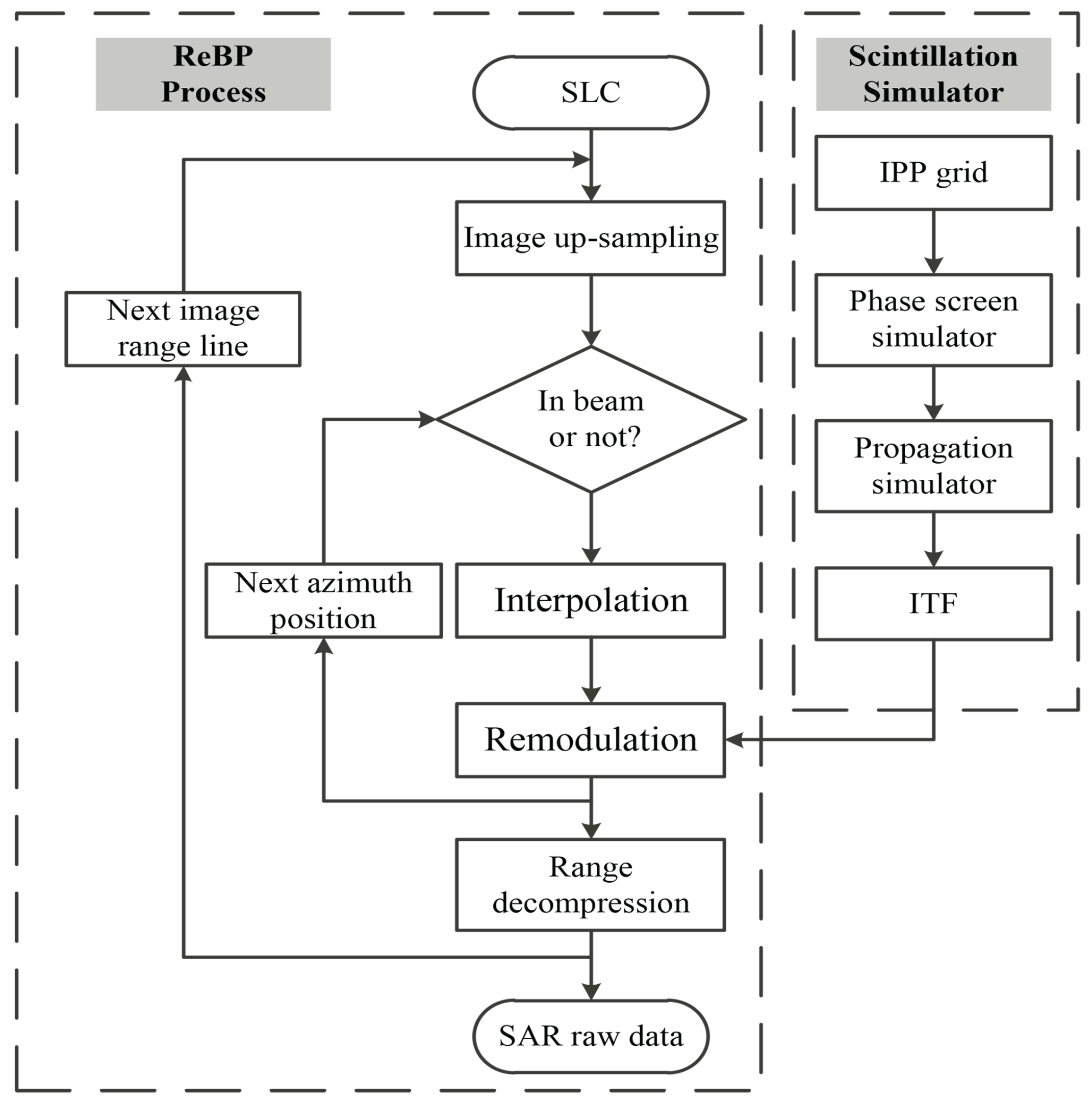
4. The ReBP-Based Scintillation Simulator for Sliding Spotlight Mode
4.1. Basic of Scintillation Simulator
4.2. The Modified Propagation Simulator for Sliding Spotlight Mode
4.3. The Modified Phase Screen Simulator for Sliding Spotlight Mode
4.4. The Structure of ReBP-Based Scintillation Simulator
5. Simulation
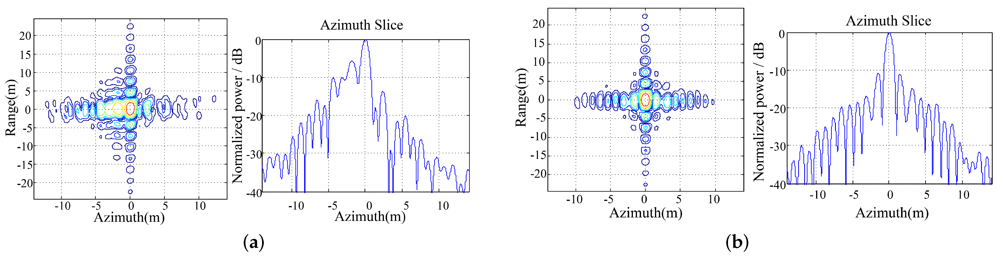
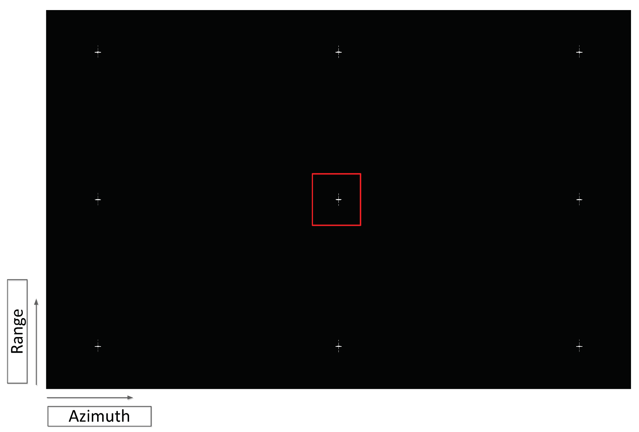
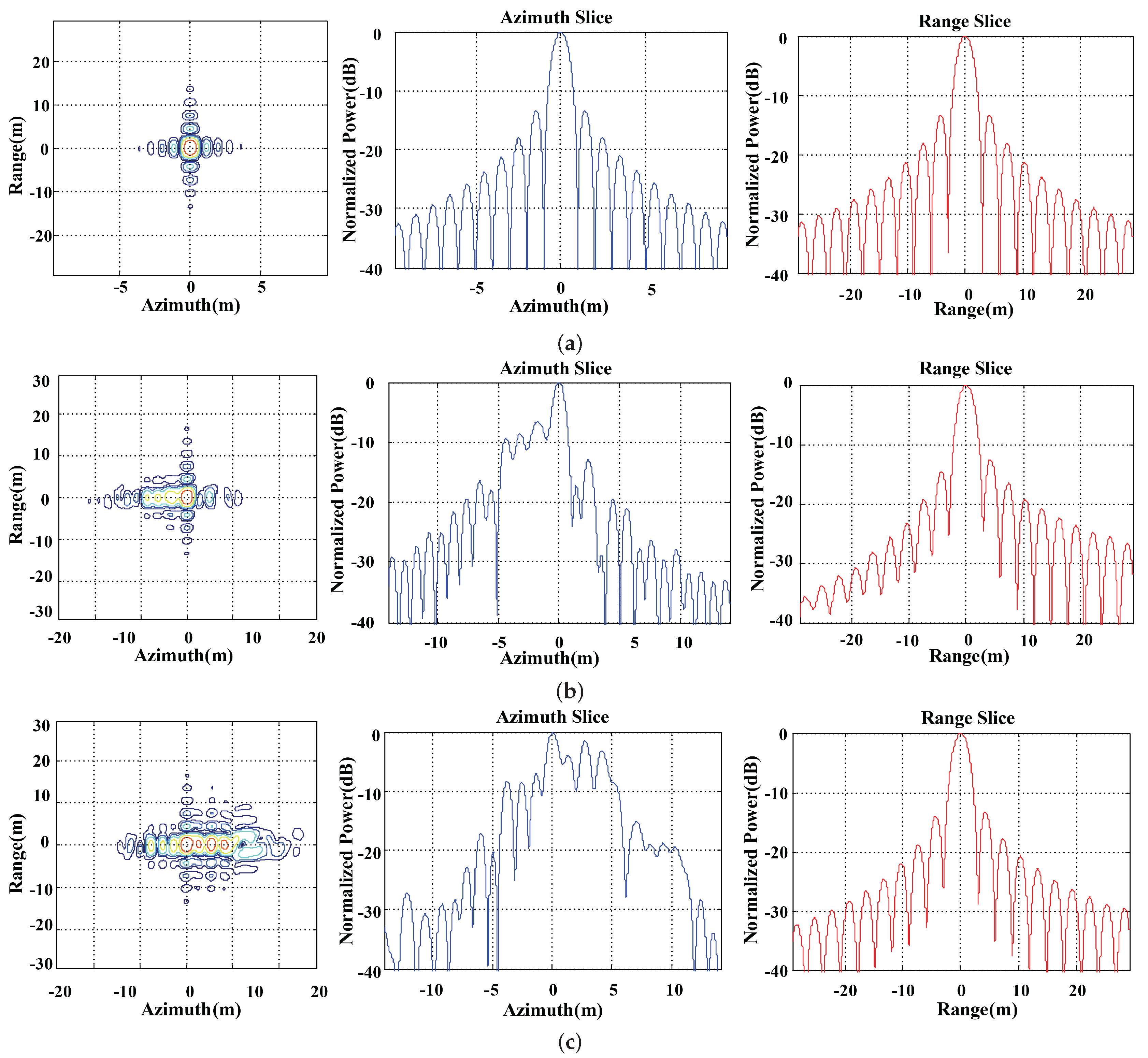
5.1. Point Target Simulation
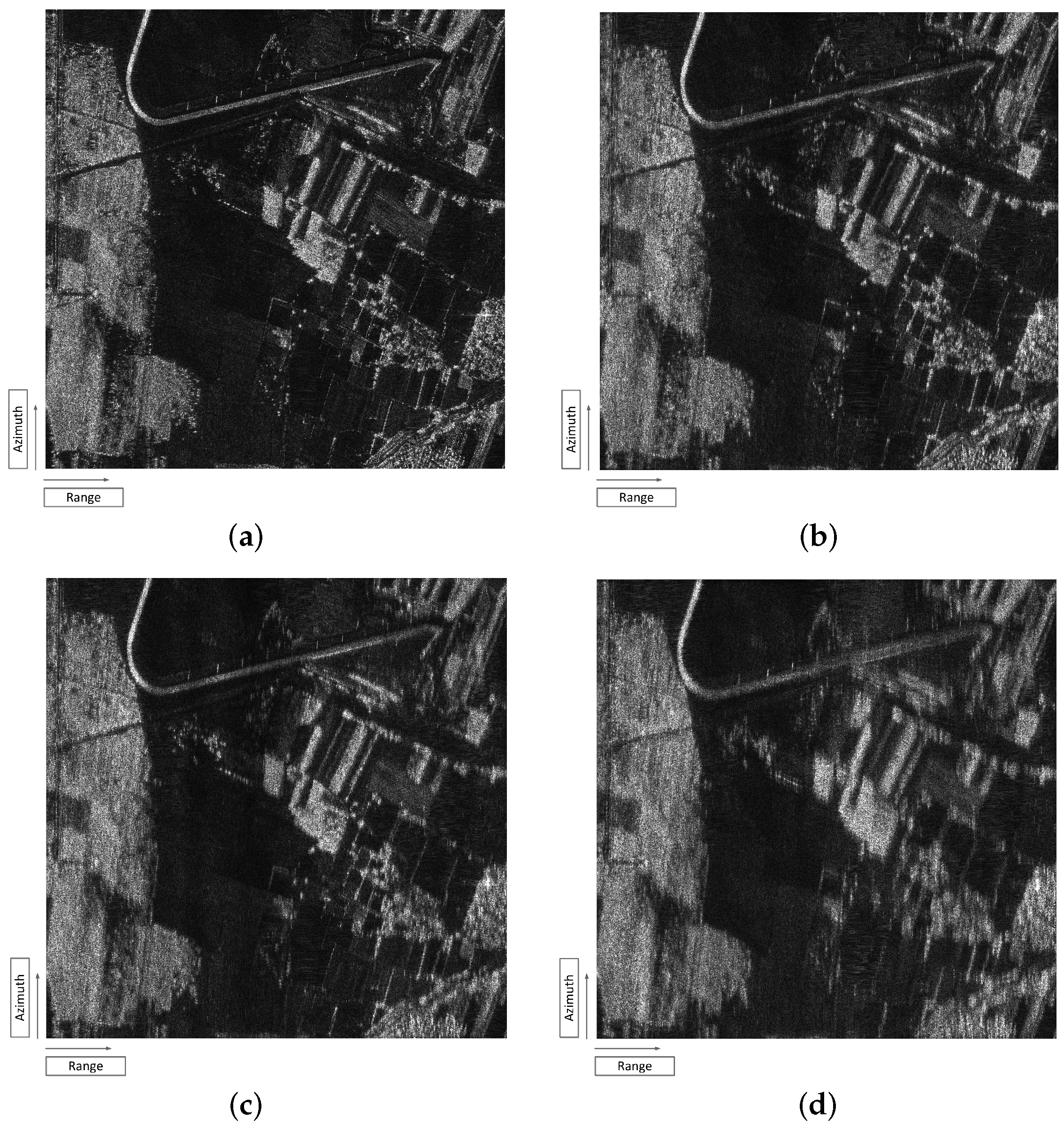
5.2. Extended Target Simulation
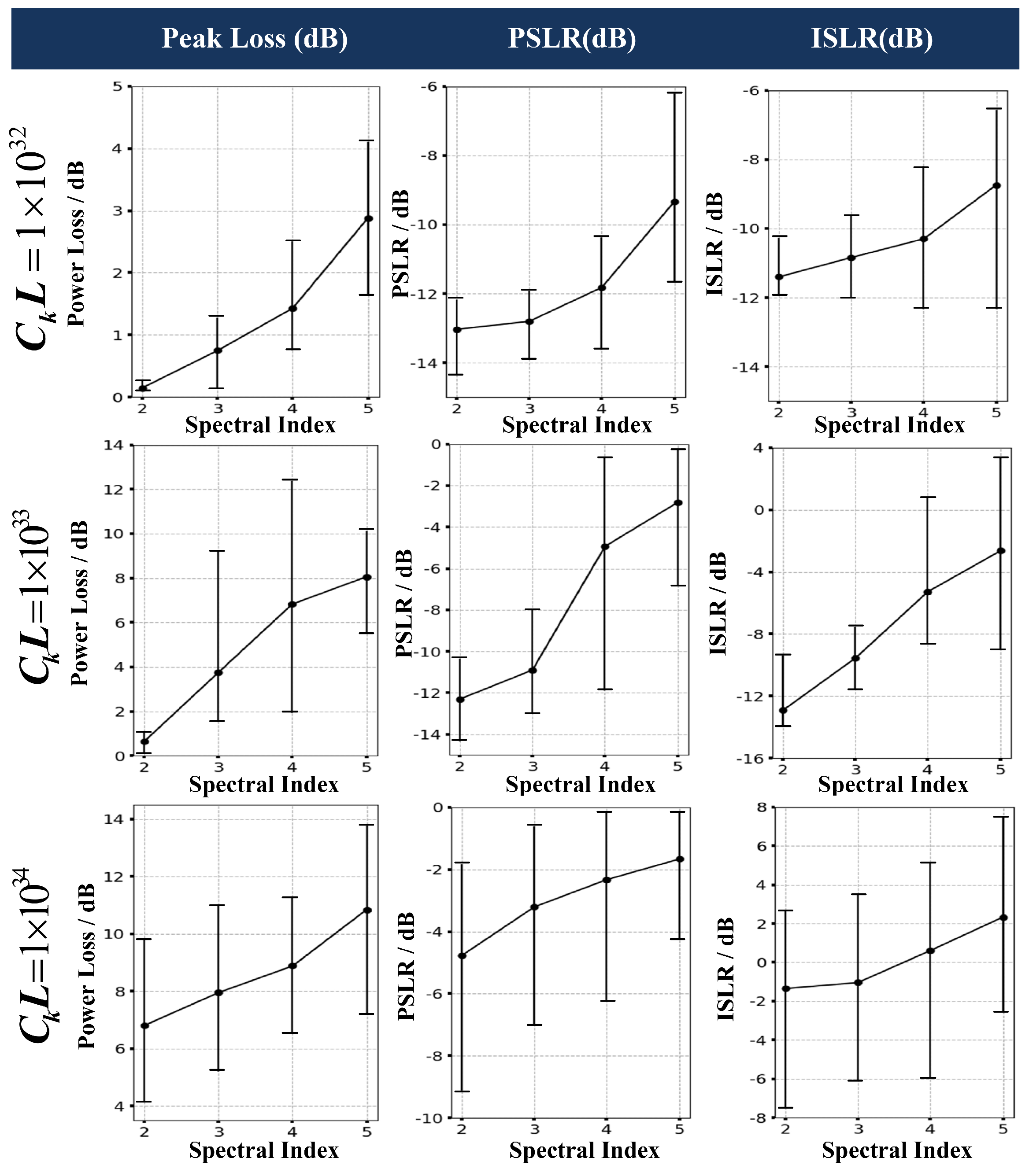
5.3. Monte-Carlo Simulation
6. Conclusions
Author Contributions
Funding
Conflicts of Interest
References
- Rignot, E.; Zimmermann, J.R.; Vanzyl, J.J. Spaceborne applications of P-band imaging radars for measuring forest biomass. IEEE Trans. Geosci. Remote Sens. 1995, 33, 1162–1169. [Google Scholar] [CrossRef]
- Toan, T.L.; Beaudoin, A.; Riom, J.; Guyon, D. Relating forest biomass to SAR data. IEEE Trans. Geosci. Remote Sens. 1992, 30, 403–411. [Google Scholar] [CrossRef]
- Dobson, M.C.; Ulaby, F.T.; Toan, T.L.; Beaudoin, A. Dependence of radar backscatter on coniferous forest biomass. IEEE Trans. Geosci. Remote Sens. 1992, 30, 412–415. [Google Scholar] [CrossRef]
- Arcioni, M.; Bensi, P.; Davidson, M.W.; Drinkwater, M.; Fois, F.; Lin, C.C.; Meynart, R.; Scipal, K.; Silvestrin, P. ESA’S BIOMASS mission candidate system and payload overview. In Proceedings of the IEEE International Geoscience and Remote Sensing Symposium, Munich, Germany, 22–27 July 2012; pp. 5530–5533. [Google Scholar]
- Mancon, S.; Giudici, D.; Tebaldini, S. The ionospheric effects mitigation in the BIOMASS mission exploiting multi-squint coherence. In Proceedings of the 12th European Conference on Synthetic Aperture Radar, Aachen, Germany, 4–7 June 2018; pp. 1–6. [Google Scholar]
- Meyer, F.; Bamler, R.; Jakowski, N.; Fritz, T. The Potential of Low-Frequency SAR Systems for Mapping Ionospheric TEC Distributions. IEEE Geosci. Remote Sens. Lett. 2006, 3, 560–564. [Google Scholar] [CrossRef]
- Rogers, N.C.; Quegan, S.; Kim, J.S.; Papathanassiou, K.P. Impacts of ionospheric scintillation on the BIOMASS P-band satellite SAR. IEEE Trans. Geosci. Remote Sens. 2014, 52, 1856–1868. [Google Scholar] [CrossRef]
- Liu, J.; Kuga, Y.; Ishimaru, A.; Pi, X.; Freeman, A. Ionospheric effects on SAR imaging: A numerical study. IEEE Trans. Geosci. Remote Sens. 2003, 41, 939–947. [Google Scholar]
- Xu, Z.W.; Wu, J.; Wu, Z.S. Potential effects of the ionosphere on space-based SAR imaging. IEEE Trans. Geosci. Remote Sens. 2008, 56, 1968–1975. [Google Scholar]
- Mittermayer, J.; Moreira, A.; Loffeld, O. Spotlight SAR data processing using the frequency scaling algorithm. IEEE Trans. Geosci. Remote Sens. 1999, 37, 2198–2214. [Google Scholar] [CrossRef]
- Eldhuset, K. Ultra high resolution spaceborne SAR processing. IEEE Trans. Aerosp. Electron. Syst. 2004, 40, 370–378. [Google Scholar] [CrossRef]
- Wang, P.; Liu, W.; Chen, J.; Niu, M.; Yang, W. A high-order imaging algorithm for high-resolution spaceborne SAR based on a modified equivalent squint range model. IEEE Trans. Geosci. Remote Sens. 2015, 53, 1225–1235. [Google Scholar] [CrossRef]
- He, F.; Chen, Q.; Dong, Z.; Sun, Z. Processing of Ultrahigh-Resolution Spaceborne Sliding Spotlight SAR Data on Curved Orbit. IEEE Trans. Aerosp. Electron. Syst. 2013, 49, 819–839. [Google Scholar] [CrossRef]
- Xu, Z.W.; Wu, J.; Wu, Z.S. A survey of ionospheric effects on space-based radar. Waves Random Media 2004, 14, S189–S273. [Google Scholar] [CrossRef]
- Meyer, F.J. Performance Requirements for Ionospheric Correction of Low-Frequency SAR Data. IEEE Trans. Geosci. Remote Sens. 2011, 49, 3694–3702. [Google Scholar] [CrossRef]
- Mannix, C.R.; Belcher, D.P.; Cannon, P.S.; Angling, M.J. Using GNSS signals as a proxy for SAR signals: Correcting ionospheric defocusing. Radio Sci. 2016, 51, 60–70. [Google Scholar] [CrossRef]
- Xiao, W.; Liu, W.; Sun, G. Modernization milestone: BeiDou M2-S initial signal analysis. GPS Solut. 2015, 20, 125–133. [Google Scholar] [CrossRef]
- Azcueta, M.; Tebaldini, S. Non-Cooperative Bistatic SAR Clock Drift Compensation for Tomographic Acquisitions. Remote Sens. 2017, 9, 1087. [Google Scholar] [CrossRef]
- Ishimaru, A.; Kuga, Y.; Liu, J.; Kim, Y.; Freeman, T. Ionospheric effects on synthetic aperture radar imaging at 100 MHz to 2 GHz. Radio Sci. 1999, 34, 257–268. [Google Scholar] [CrossRef]
- Li, L.L.; Li, F. SAR imaging degradation by ionospheric irregularities based on TFTPCF analysis. IEEE Trans. Geosci. Remote Sens. 2007, 45, 1123–1130. [Google Scholar] [CrossRef]
- Belcher, D.; Cannon, P. Amplitude scintillation effects on SAR. IET Radar Sonar Navig. 2014, 8, 658–666. [Google Scholar] [CrossRef]
- Meyer, F.J. A review of ionospheric effects in low-frequency SAR–Signals, correction methods, and performance requirements. In Proceedings of the 2010 IEEE International Geoscience and Remote Sensing Symposium, Honolulu, HI, USA, 25–30 July 2010; pp. 29–32. [Google Scholar]
- Wang, C.; Zhang, M.; Xu, Z.W.; Chen, C.; Sheng, D.S. Effects of anisotropic ionospheric irregularities on space-Borne SAR imaging. IEEE Trans. Geosci. Remote Sens. 2014, 62, 4664–4673. [Google Scholar] [CrossRef]
- Meyer, F.; Chotoo, K.; Chotoo, S.; Huxtable, B.; Carrano, C. The influence of equatorial scintillation on L-band SAR image quality and phase. IEEE Trans. Geosci. Remote Sens. 2016, 54, 869–880. [Google Scholar] [CrossRef]
- Hu, C.; Li, Y.; Dong, X.; Wang, R.; Ao, D. Performance Analysis of L-Band Geosynchronous SAR Imaging in the Presence of Ionospheric Scintillation. IEEE Trans. Geosci. Remote Sens. 2017, 55, 159–172. [Google Scholar] [CrossRef]
- Ji, Y.F.; Zhang, Q.L.; Zhang, Y.S.; Dong, Z. L-band geosynchronous SAR imaging degradations imposed by ionospheric irregularities. China Sci. Inf. Sci. 2017, 60, 060308. [Google Scholar] [CrossRef]
- Carrano, C.S.; Groves, K.M.; Caton, R.G. Simulating the impacts of ionospheric scintillation on L band SAR image formation. Radio Sci. 2012, 47, RS0L20. [Google Scholar] [CrossRef]
- Li, D.; Rodriguez-Cassola, M.; Prats-Iraola, P.; Wu, M.; Moreira, A. Reverse Backprojection Algorithm for the Accurate Generation of SAR Raw Data of Natural Scenes. IEEE Geosci. Remote Sens. Lett. 2017, 14, 2072–2076. [Google Scholar] [CrossRef]
- Rino, C.L. A power law phase screen model for ionospheric scintillation 2. Strong scatter. Radio Sci. 1979, 14, 1147–1155. [Google Scholar] [CrossRef]


| Parameters | Symbol | Value |
|---|---|---|
| Scintillation strength | ||
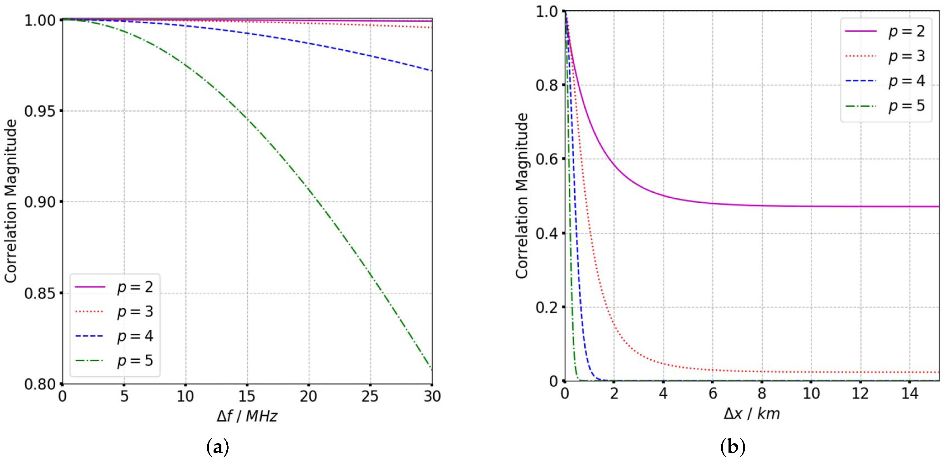
| Spectral index | p | 3 |
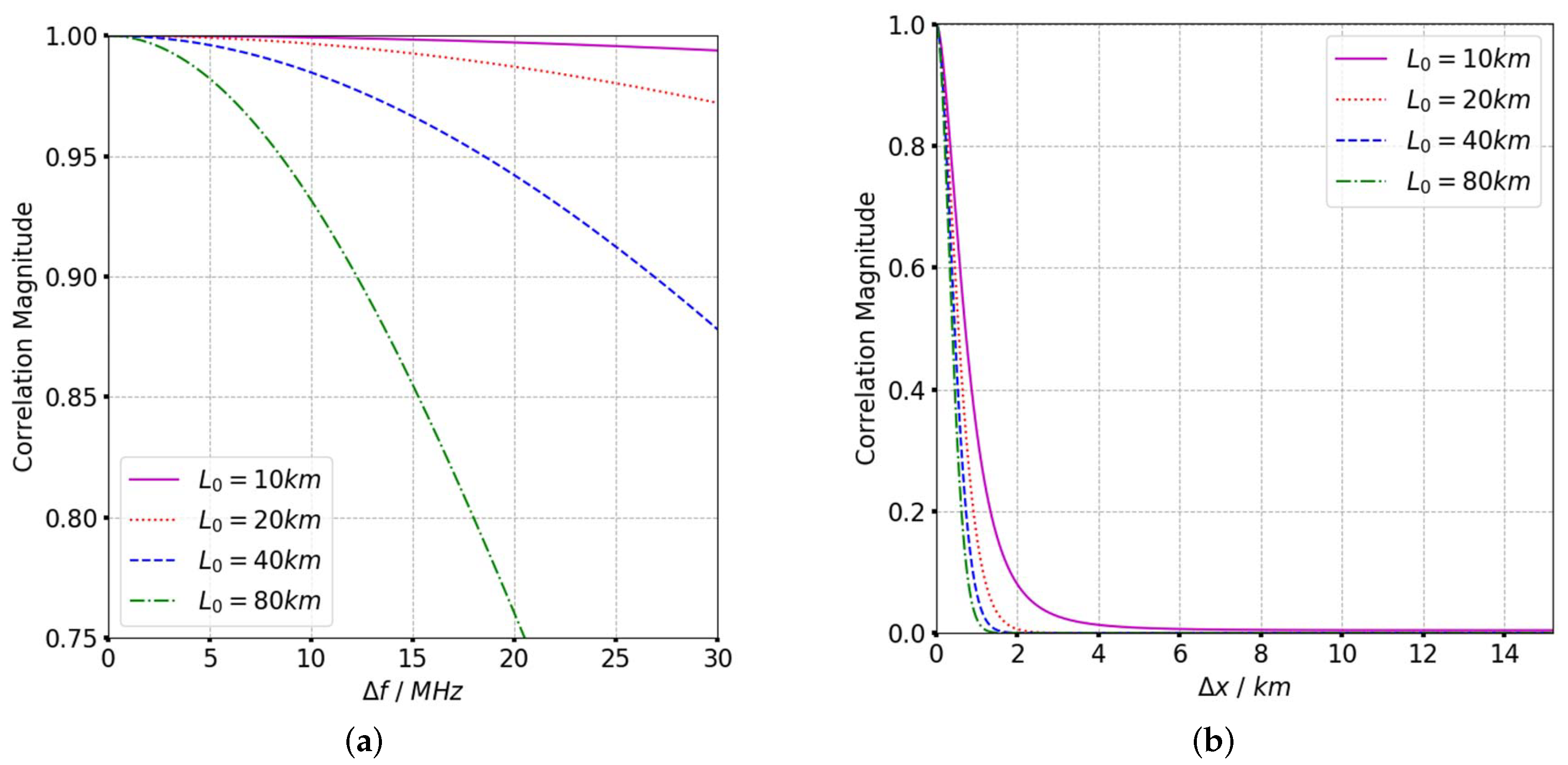
| Outer scale | 10 km | |
| Irregularity structure scale | a/b | 10/1 |
| Parameters | Value | Unit |
|---|---|---|
| Carrier frequency | 0.6 | GHz |
| Bandwidth | 60 | MHz |
| Altitude of radar | 700 | km |
| Scanning angular velocity() | −0.0055 | rad/s |
| Semi-major Axis | 7071 | km |
| Inclination | 98.6 | deg |
| The Argument of Latitude | 40 | deg |
| Peak Loss/dB | PSLR/dB | ISLR/dB | ||||||||||
|---|---|---|---|---|---|---|---|---|---|---|---|---|
| Spectral Index | 2 | 3 | 4 | 5 | 2 | 3 | 4 | 5 | 2 | 3 | 4 | 5 |
| Sliding spotlight | 6.81 | 7.95 | 8.88 | 10.84 | −4.77 | −3.21 | −2.33 | −1.67 | −1.35 | −1.04 | 0.61 | 2.33 |
| Stripmap | 2.08 | 4.41 | 6.20 | 7.87 | −6.57 | −4.39 | −2.76 | −1.99 | −3.96 | −2.73 | −0.45 | 0.36 |
© 2019 by the authors. Licensee MDPI, Basel, Switzerland. This article is an open access article distributed under the terms and conditions of the Creative Commons Attribution (CC BY) license (http://creativecommons.org/licenses/by/4.0/).
Share and Cite
Yu, L.; Zhang, Y.; Zhang, Q.; Ji, Y.; Dong, Z. Performance Analysis of Ionospheric Scintillation Effect on P-Band Sliding Spotlight SAR System. Sensors 2019, 19, 2161. https://doi.org/10.3390/s19092161
Yu L, Zhang Y, Zhang Q, Ji Y, Dong Z. Performance Analysis of Ionospheric Scintillation Effect on P-Band Sliding Spotlight SAR System. Sensors. 2019; 19(9):2161. https://doi.org/10.3390/s19092161
Chicago/Turabian StyleYu, Lei, Yongsheng Zhang, Qilei Zhang, Yifei Ji, and Zhen Dong. 2019. "Performance Analysis of Ionospheric Scintillation Effect on P-Band Sliding Spotlight SAR System" Sensors 19, no. 9: 2161. https://doi.org/10.3390/s19092161
APA StyleYu, L., Zhang, Y., Zhang, Q., Ji, Y., & Dong, Z. (2019). Performance Analysis of Ionospheric Scintillation Effect on P-Band Sliding Spotlight SAR System. Sensors, 19(9), 2161. https://doi.org/10.3390/s19092161