A Rubber-Tapping Robot Forest Navigation and Information Collection System Based on 2D LiDAR and a Gyroscope


Abstract
:1. Introduction
2. Materials and Methods
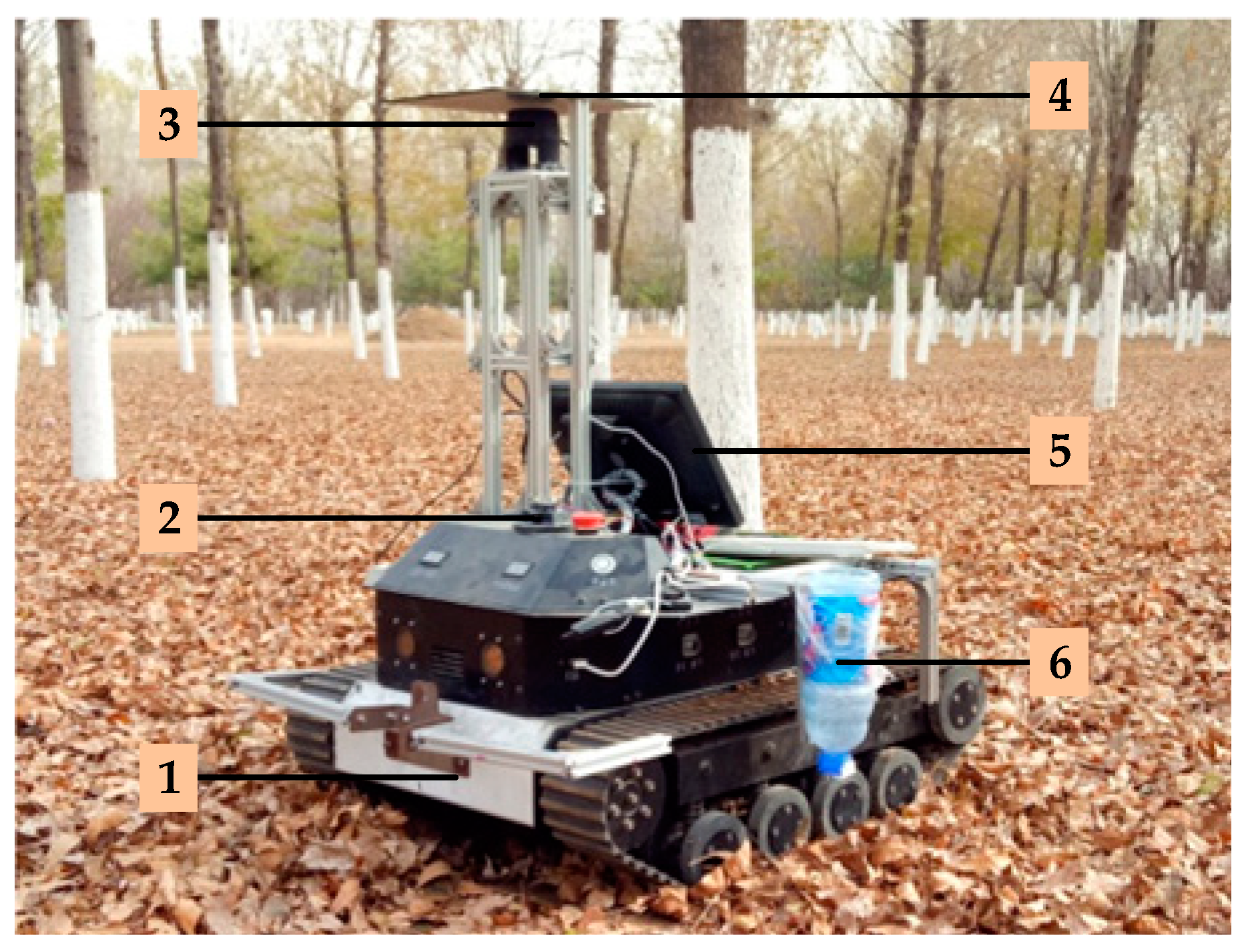
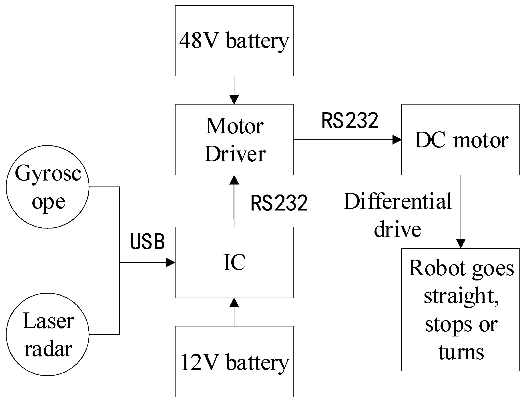
2.1. System Composition
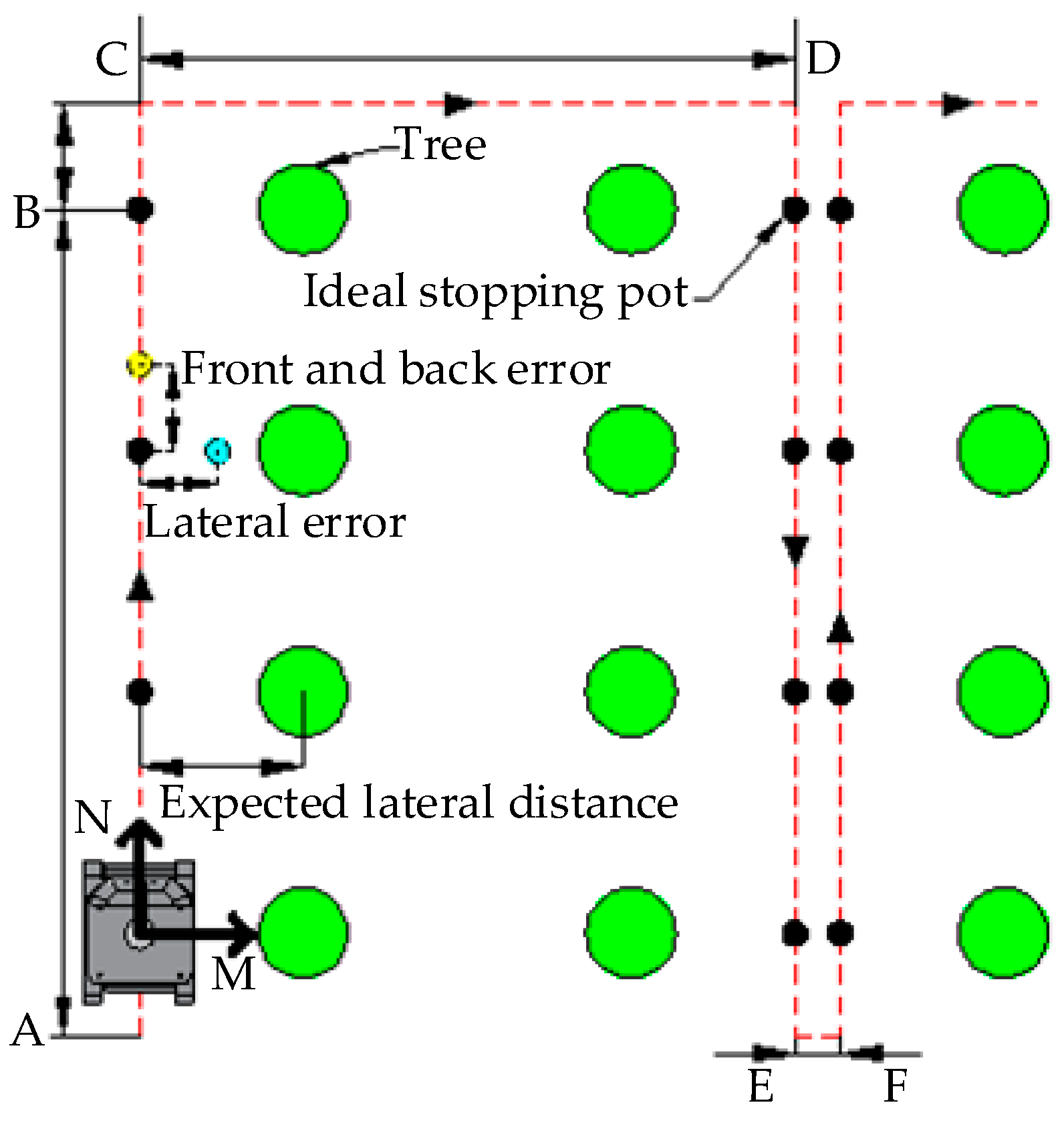
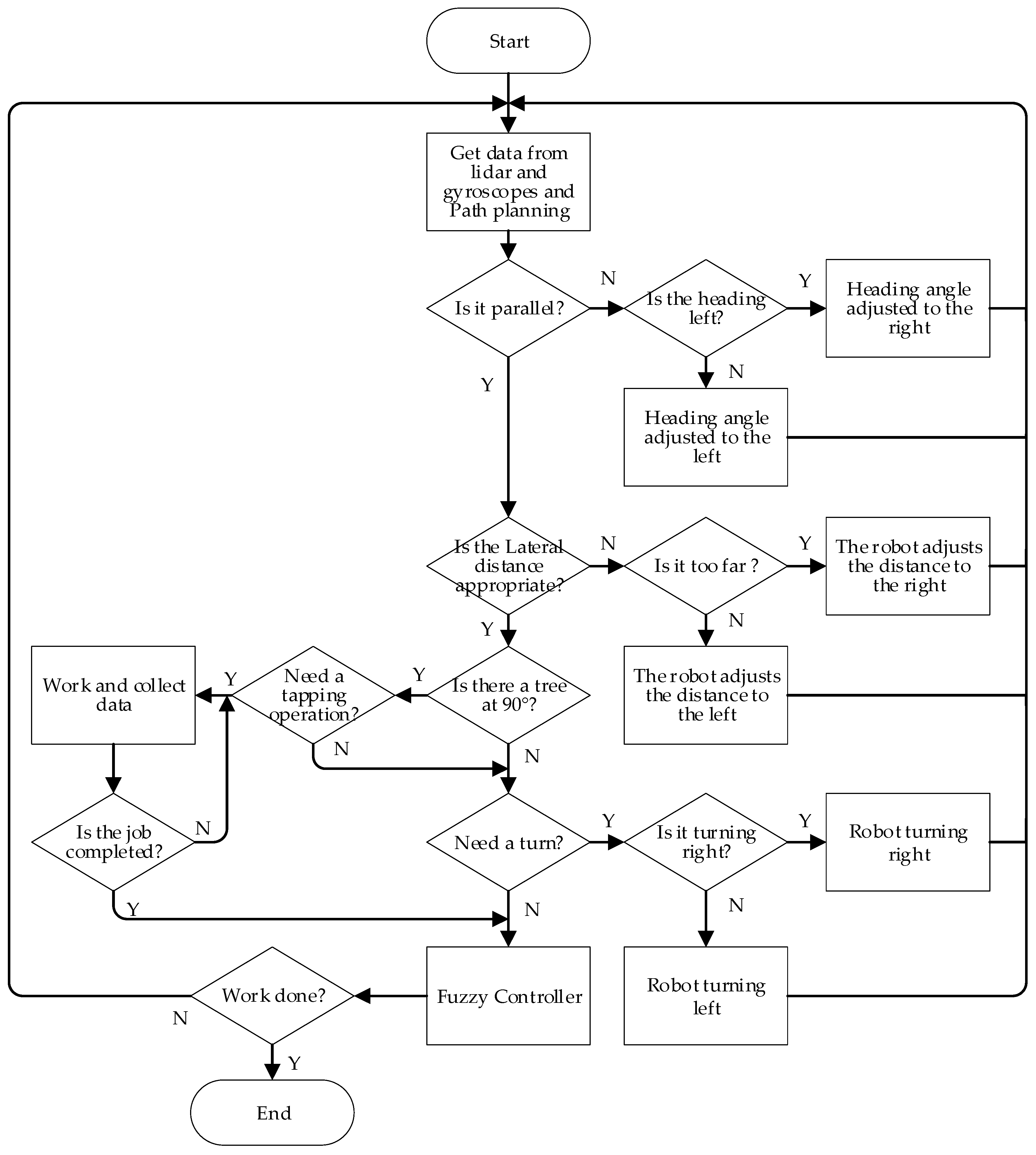
2.2. Navigation Strategy
- Autonomously navigate along one row with a fixed lateral distance;
- Stop at the designed spot in front of trees;
- Turn from one row into another;
- Information collection.
2.3. Navigation Phases
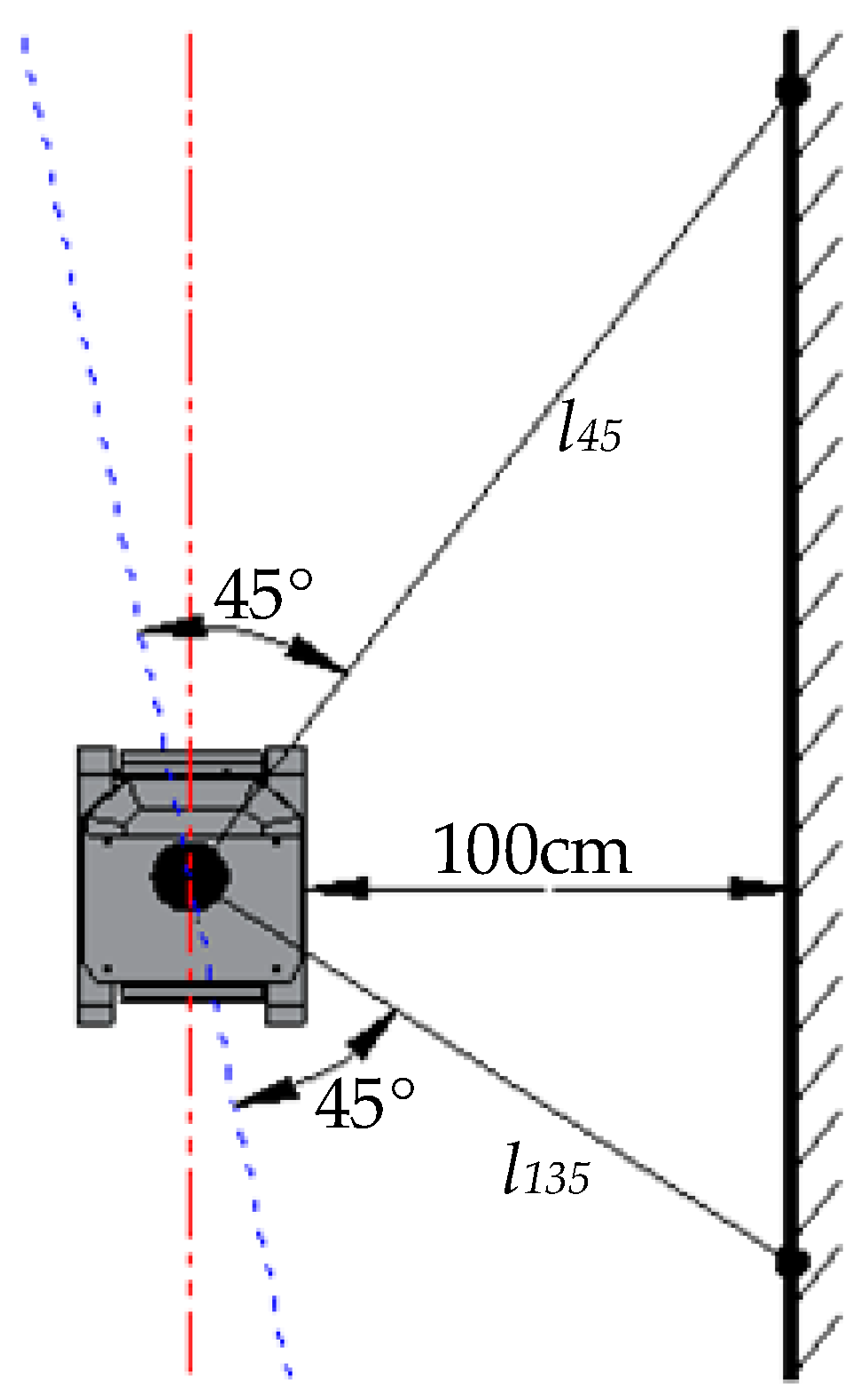
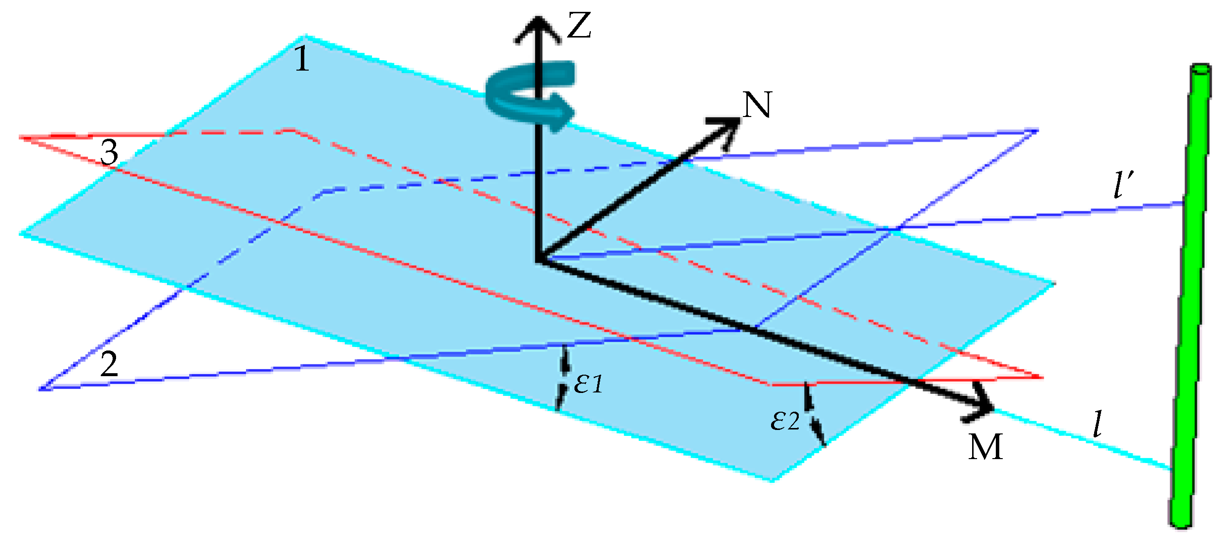
2.4. Calibration of the Installed Location of LiDAR
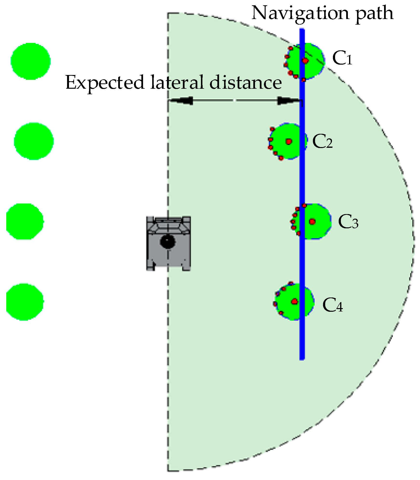
2.5. Navigation Path Generation
- (1)
- The distance difference between two points and the LiDAR is less than the threshold δ1 (δ1 is determined by the diameter), i.e.,
- (2)
- The angle difference between two points and the LiDAR is less than the threshold δ2 (δ2 is determined by the diameter and the distance between the robot and the tree row), i.e.,
- (3)
- The distance difference between two points and the center line of the robot is less than the threshold δ3 (δ3 is determined by the row spacing), i.e.,
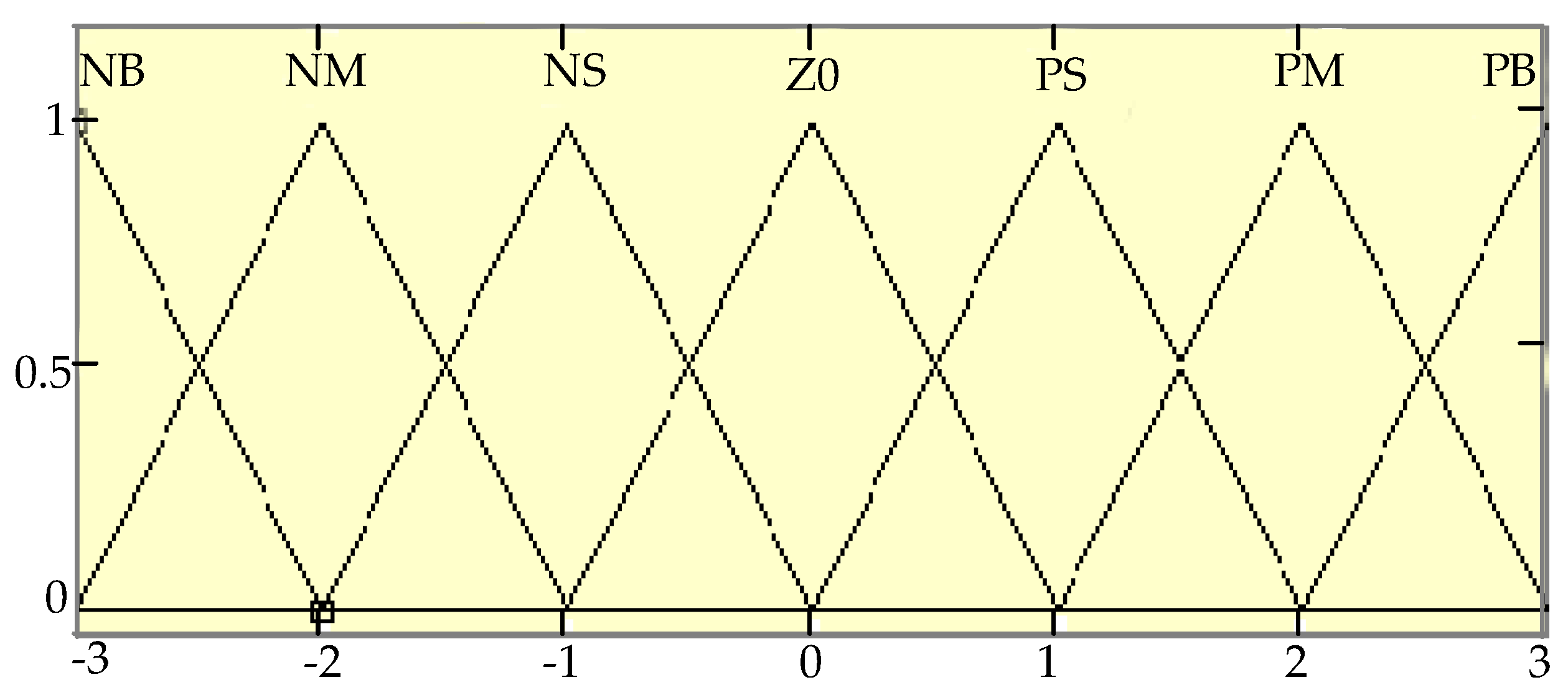
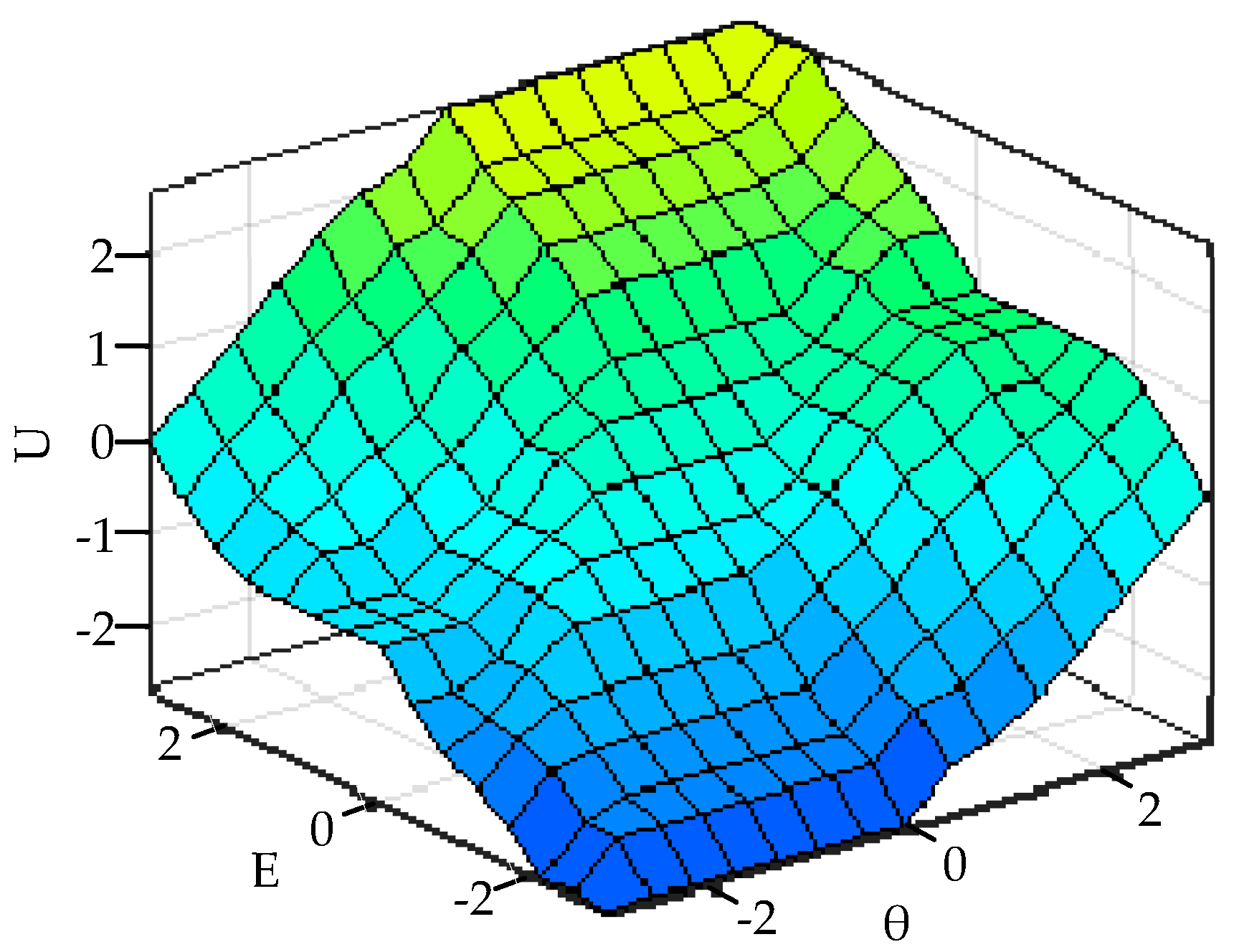
2.6. Design of the Fuzzy Controller
2.7. Location of the Robot
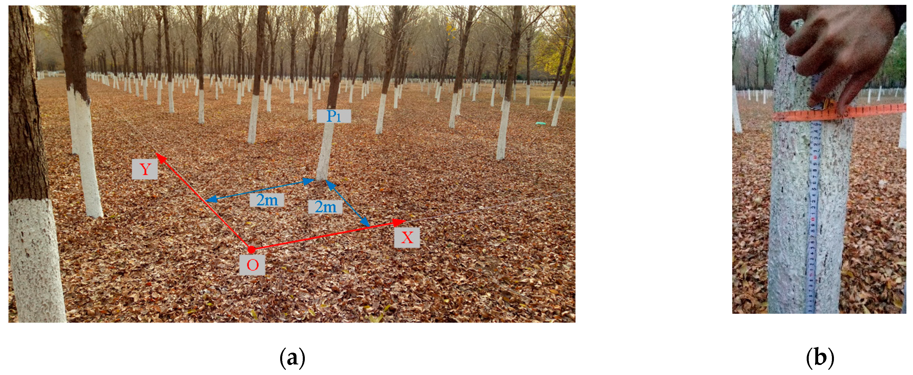
2.8. Information Collection
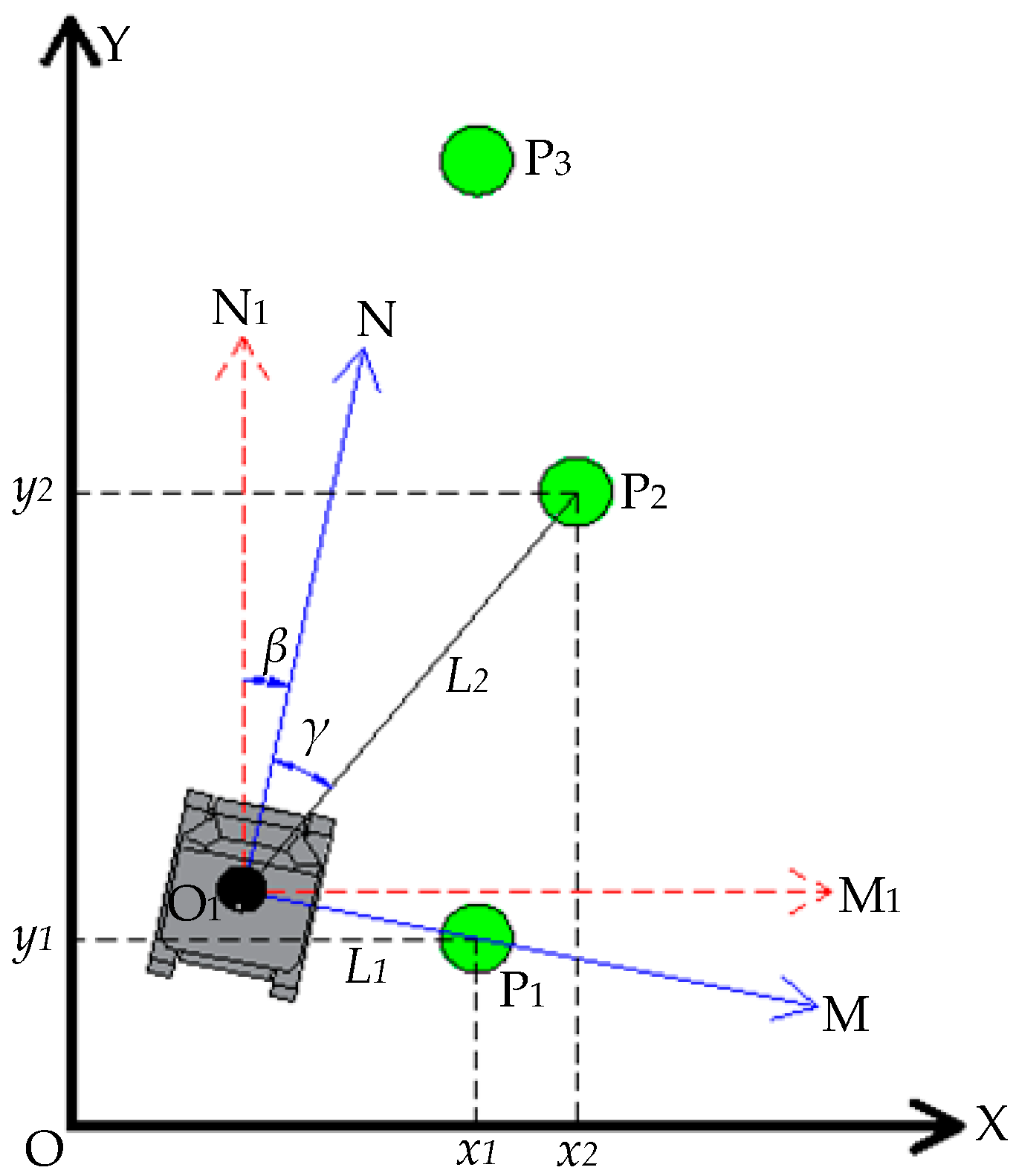
2.8.1. Calculation of Tree Position
2.8.2. Calculation of Tree Radius
3. Results
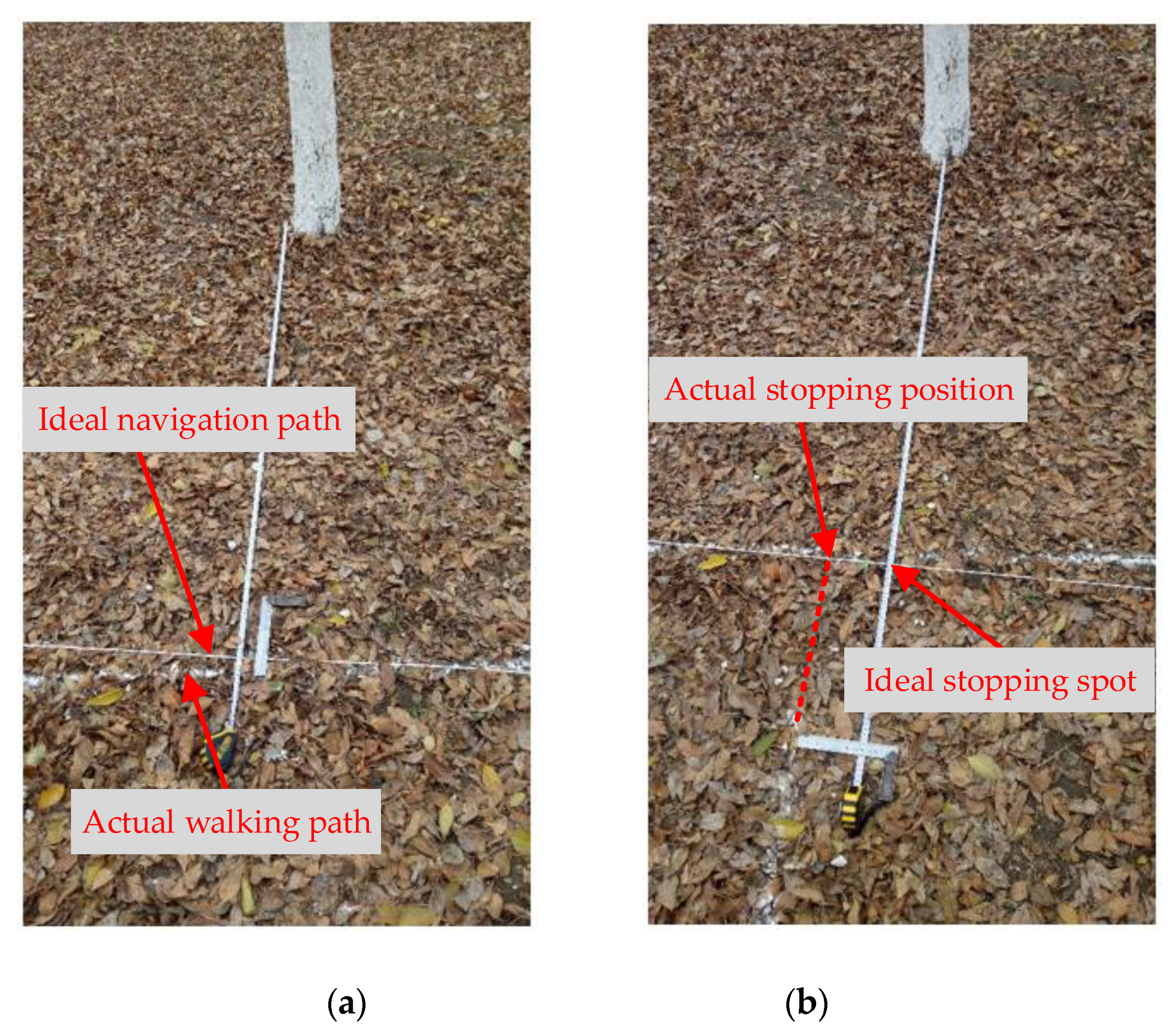
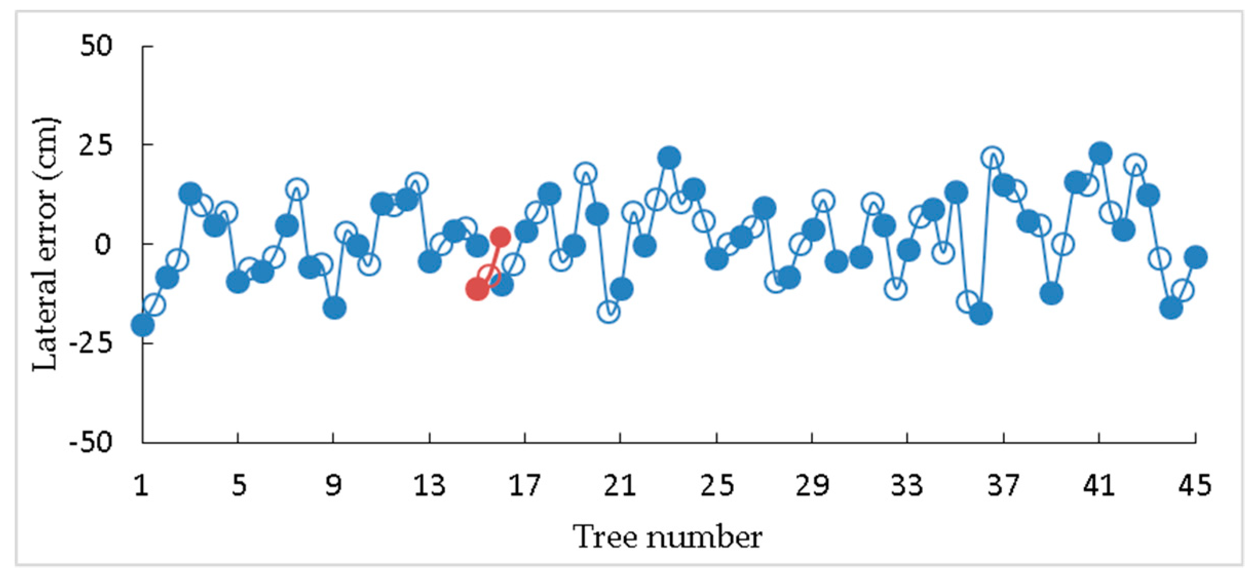
3.1. Navigation Results Analysis
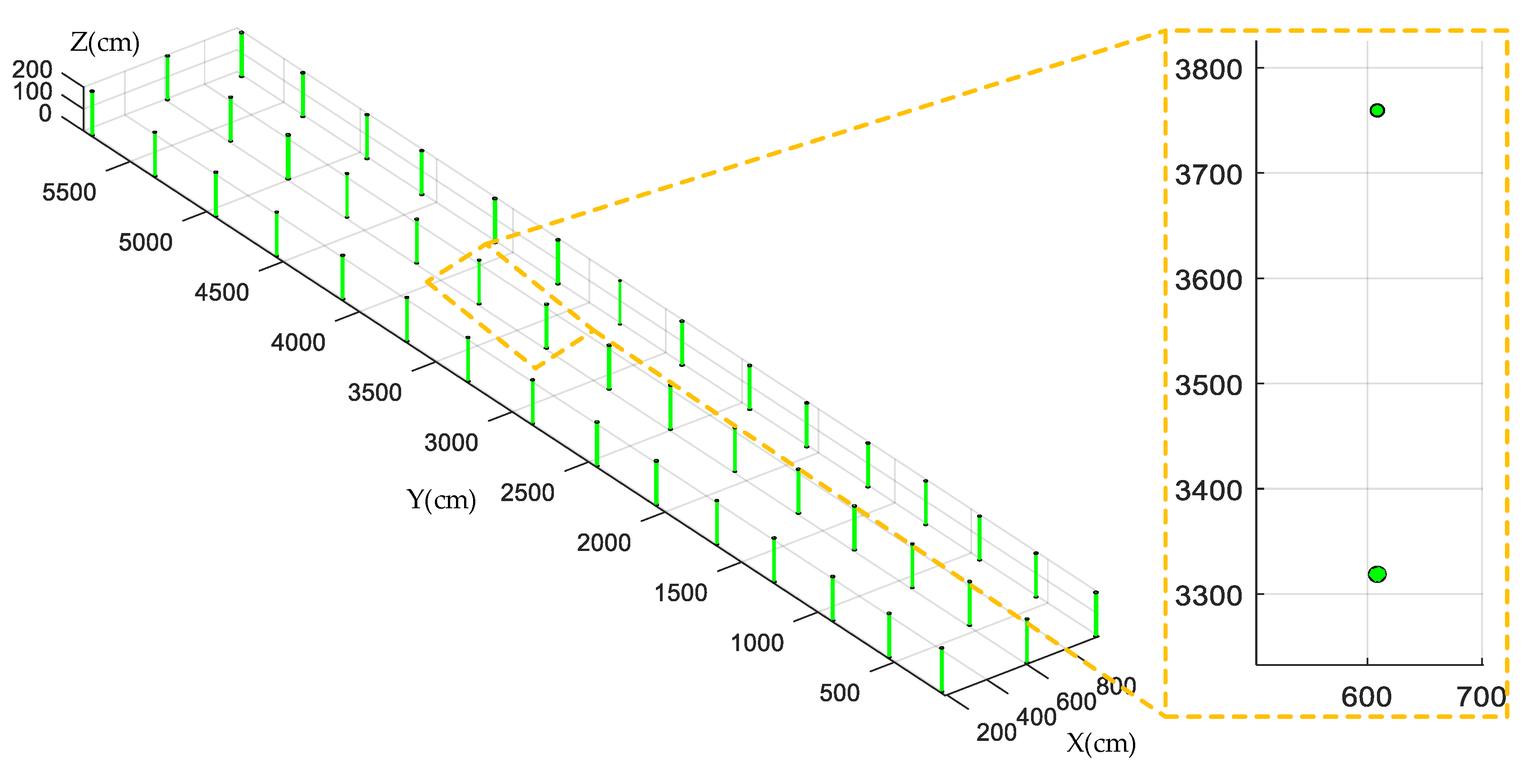
3.2. Mapping Results Analysis
4. Conclusions
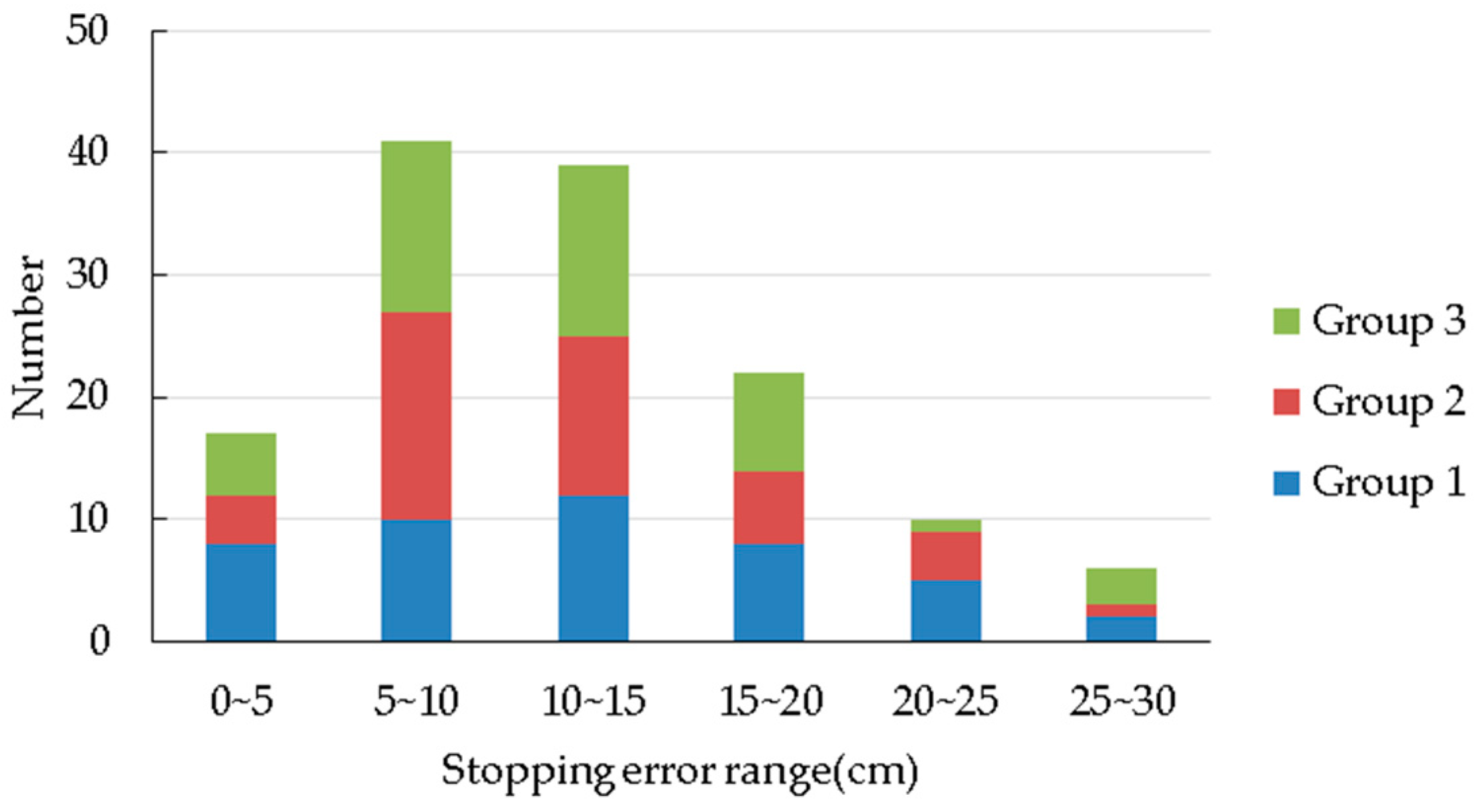
- A method for forest navigation for an automatic rubber tapping platform was proposed in this paper. Instead of relying on GPS and prior maps, the method makes the robot walk along one row at a fixed lateral distance, stop at a fixed point, and turn from one row into another, only using low-cost two-dimensional (2D) LiDAR and a gyroscope. The root mean square (RMS) lateral errors with three repeated tests are 10.31 cm, 10.32 cm, and 9.37 cm, respectively, which shows that the method has great path tracking performance. The method provides better fixed-point stopping with average stopping errors of 12.62 cm, 11.98 cm, and 11.64 cm, respectively, which meets the requirements of forest navigation for a rubber-tapping robot.
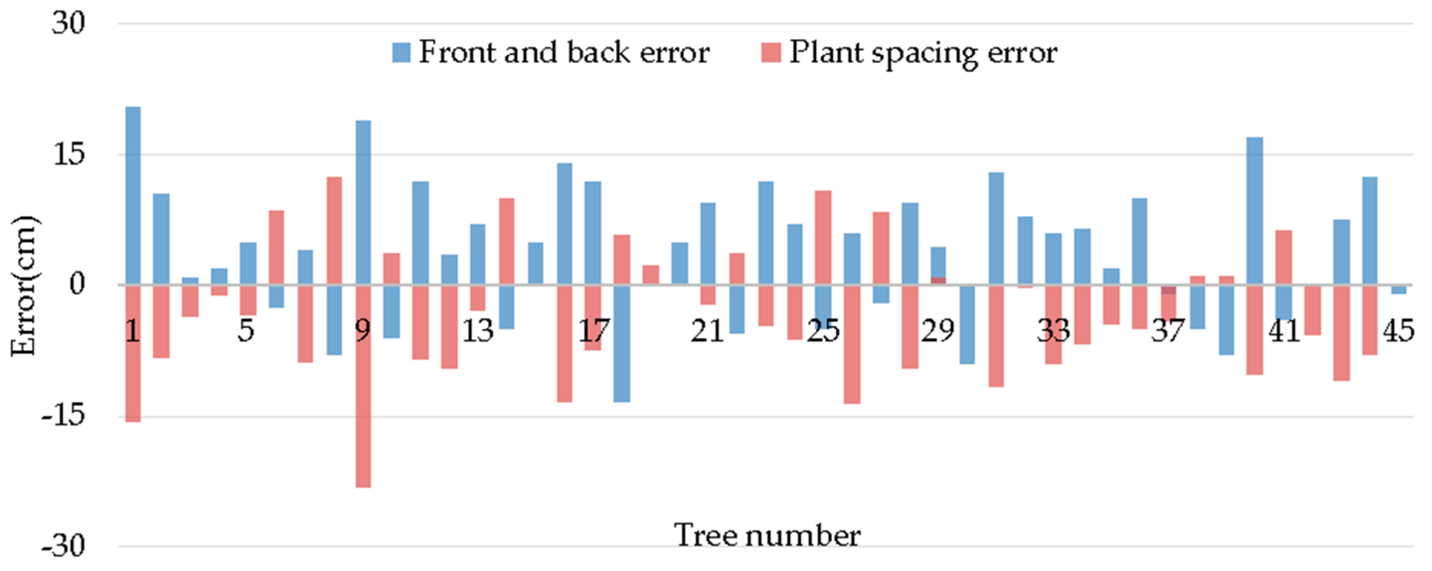
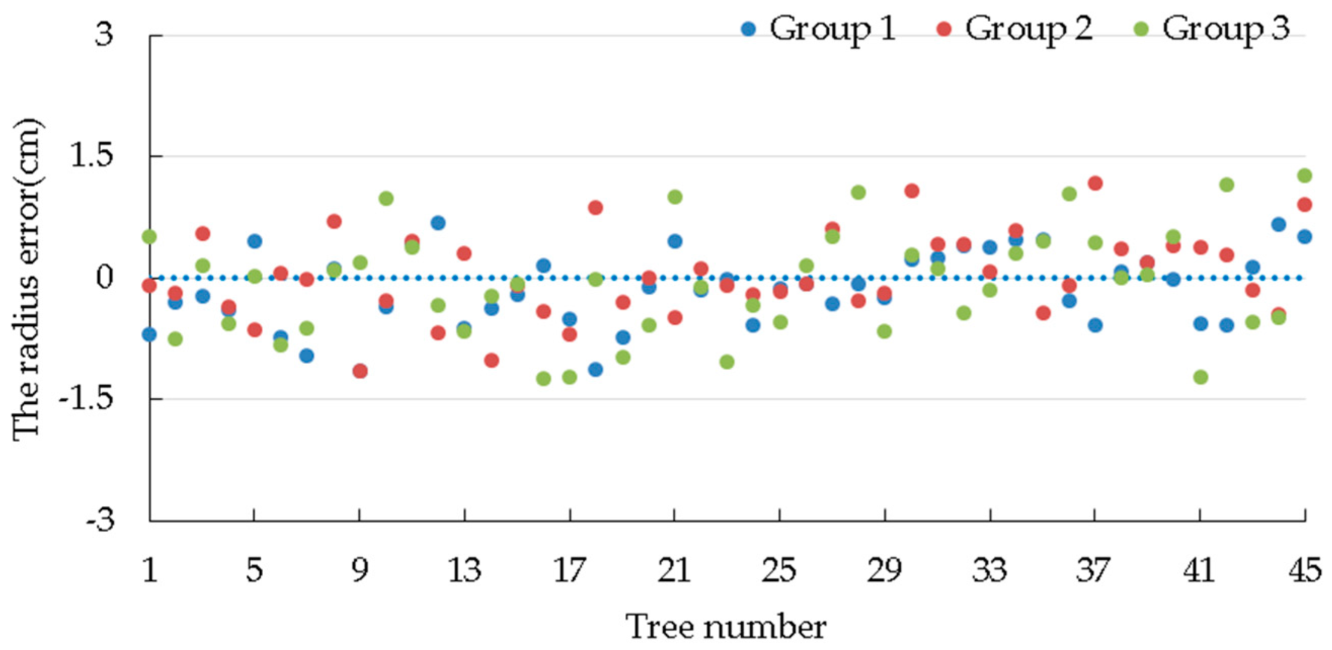
- A method of collecting forest information in real time during navigation was developed. Among the information collected on the forest during the tests, the RMS radius errors are less than 0.66 cm, and the RMS plant spacing errors less than 11.31 cm. The results show that the collected data could reflect the true parameters of the forest well.
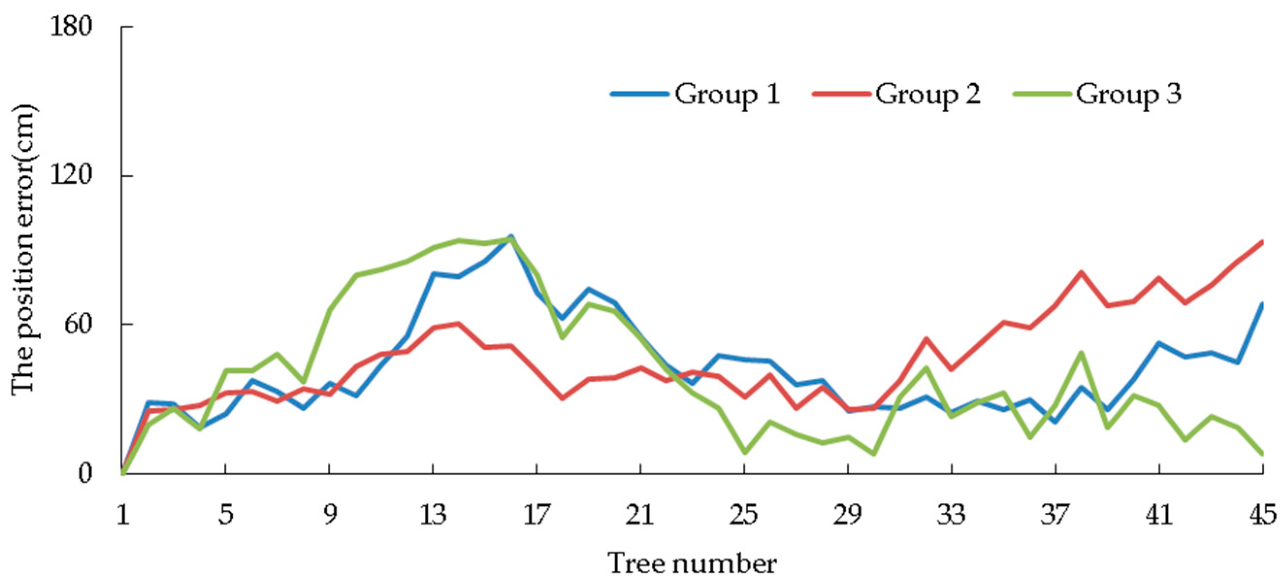
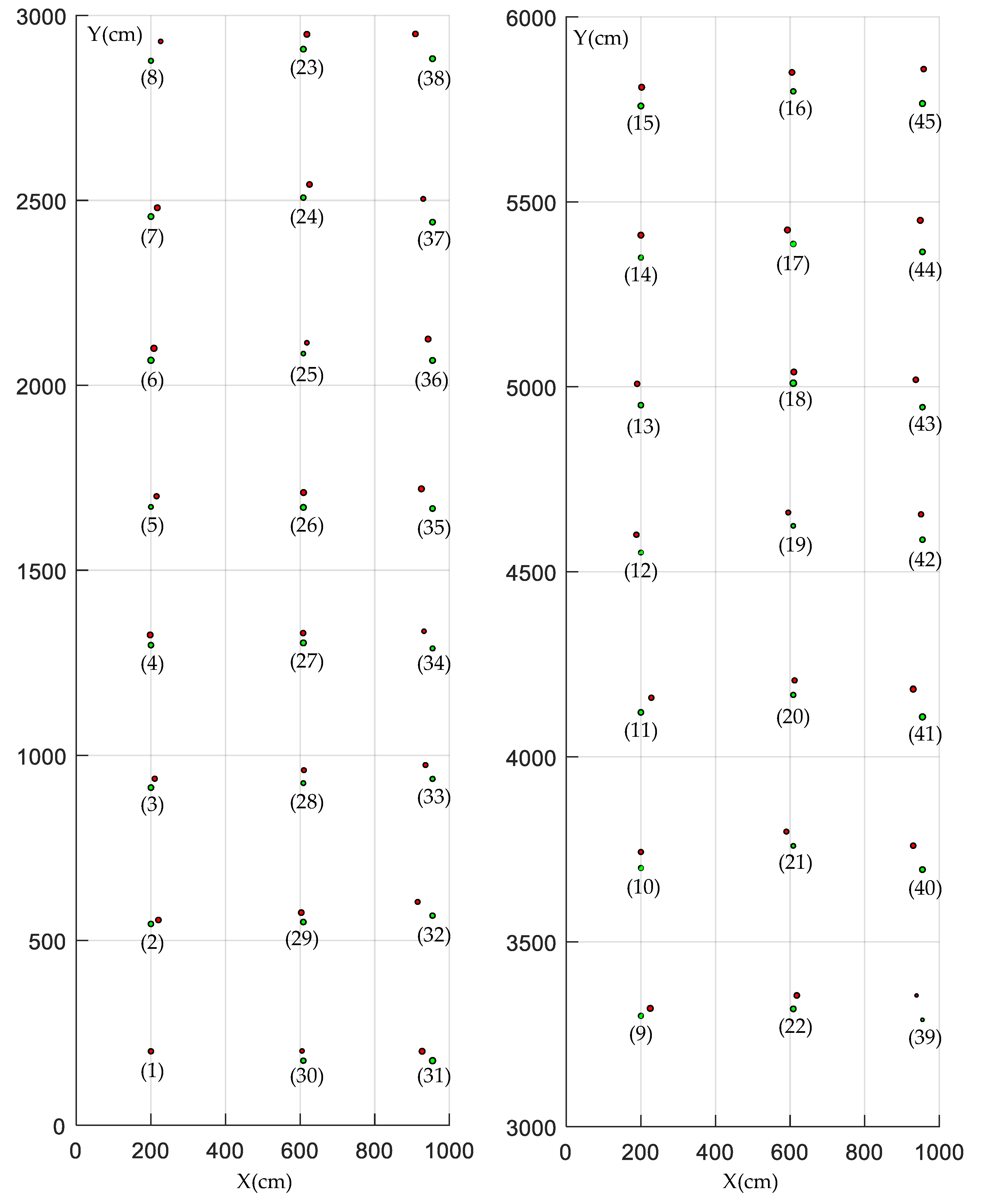
- A method for constructing a geometric feature map based on the collected information was introduced. In the constructed geometric feature map, the average position errors are 43.00 cm, 46.48 cm, and 40.40 cm respectively, indicating that the map containing information on the forest not only benefits the informatization and precision management of trees, but also provides references for navigating a robot based on prior maps.
Author Contributions
Funding
Conflicts of Interest
References
- Wu, C.; Ban, S.; Gao, X.; Li, W. Correlation between DNA methylation status and rubber yield and related characteristics in Hevea brasiliensis tapped at different heights. Ind. Crop Prod. 2018, 111, 563–572. [Google Scholar] [CrossRef]
- Ahrends, A.; Hollingsworth, P.M.; Ziegler, A.D.; Fox, J.M.; Chen, H.; Su, Y.; Xu, J. Current trends of rubber plantation expansion may threaten biodiversity and livelihoods. Glob. Environ. Change 2015, 34, 48–58. [Google Scholar] [CrossRef]
- Tang, C.; Yang, M.; Fang, Y.; Luo, Y.; Gao, S.; Xiao, X.; An, Z.; Zhou, B.; Zhang, B.; Tan, X.; et al. The rubber tree genome reveals new insights into rubber production and species adaptation. Nat. Plants 2016, 2, 16073. [Google Scholar] [CrossRef]
- Li, D.; Wang, X.; Deng, Z.; Liu, H.; Yang, H.; He, G. Transcriptome analyses reveal molecular mechanism underlying tapping panel dryness of rubber tree (Hevea brasiliensis). Sci. Rep. 2016, 6, 23540. [Google Scholar] [CrossRef]
- Kou, W.; Xiao, X.; Dong, J.; Gan, S.; Zhai, D.; Zhang, G.; Qin, Y.; Li, L. Mapping Deciduous Rubber Plantation Areas and Stand Ages with PALSAR and Landsat Images. Remote Sens. 2015, 7, 1048–1073. [Google Scholar] [CrossRef]
- Yan, X.; Liao, Y. Exploration of Rubber Tree Tapping Technology. In Proceedings of the 3rd National Association of Local Mechanical Engineering Academic Annual Meeting and Cross-Strait Machinery Technology Forum, Sanya, China, 11–14 October 2013; pp. 129–132. [Google Scholar]
- An, F.; Zou, Z.; Cai, X.; Wang, J.; Rookes, J.; Lin, W.; Cahill, D.; Kong, L. Regulation of HbPIP2;3, a Latex-Abundant Water Transporter, Is Associated with Latex Dilution and Yield in the Rubber Tree (Hevea brasiliensis Muell. Arg.). PLoS ONE 2015, 10, e125595. [Google Scholar] [CrossRef]
- Wei, F.; Luo, S.; Zheng, Q.; Qiu, J.; Yang, W.; Wu, M.; Xiao, X. Transcriptome sequencing and comparative analysis reveal long-term flowing mechanisms in Hevea brasiliensis latex. Gene 2015, 556, 153–162. [Google Scholar] [CrossRef] [PubMed]
- Tang, J.; Chen, Y.; Kukko, A.; Kaartinen, H.; Jaakkola, A.; Khoramshahi, E.; Hakala, T.; Hyyppä, J.; Holopainen, M.; Hyyppä, H. SLAM-Aided Stem Mapping for Forest Inventory with Small-Footprint Mobile LiDAR. Forests 2015, 6, 4588–4606. [Google Scholar] [CrossRef]
- Fan, H.; Fu, X.; Zhang, Z.; Wu, Q. Phenology-Based Vegetation Index Differencing for Mapping of Rubber Plantations Using Landsat OLI Data. Remote Sens. 2015, 7, 6041–6058. [Google Scholar] [CrossRef]
- Keicher, R.; Seufert, H. Automatic guidance for agricultural vehicles in Europe. Comput. Electron. Agric. 2000, 25, 169–194. [Google Scholar] [CrossRef]
- Wu, J.; Yang, Q.; Bao, G.; Gao, F. Algorithm of Path Navigation Line for Robot in Forestry Environment Based on Machine Vision. Trans. Chin. Soc. Agric. Mach. 2009, 40, 176–179. [Google Scholar]
- Juman, M.A.; Wong, Y.W.; Rajkumar, R.K.; Goh, L.J. A novel tree trunk detection method for oil-palm plantation navigation. Comput. Electron. Agric. 2016, 128, 172–180. [Google Scholar] [CrossRef]
- Radcliffe, J.; Cox, J.; Bulanon, D.M. Machine vision for orchard navigation. Comput. Ind. 2018, 98, 165–171. [Google Scholar] [CrossRef]
- Bengochea-Guevara, J.; Conesa-Muñoz, J.; Andújar, D.; Ribeiro, A. Merge Fuzzy Visual Servoing and GPS-Based Planning to Obtain a Proper Navigation Behavior for a Small Crop-Inspection Robot. Sensors 2016, 16, 276. [Google Scholar] [CrossRef] [PubMed]
- Liu, L.; Mei, T.; Niu, R.; Wang, J.; Liu, Y.; Chu, S. RBF-Based Monocular Vision Navigation for Small Vehicles in Narrow Space below Maize Canopy. Appl. Sci. 2016, 6, 182. [Google Scholar] [CrossRef]
- Reid, J.F.; Zhang, Q.; Noguchi, N.; Dickson, M. Agricultural automatic guidance research in North America. Comput. Electron. Agric. 2000, 25, 155–167. [Google Scholar] [CrossRef]
- Benet, B.; Lenain, R. Multi-sensor fusion method for crop row tracking and traversability operations. In Proceedings of the Conférence Axema-Eurageng 2017, Paris, France, 25 February 2017. [Google Scholar]
- Liu, S.; Atia, M.M.; Karamat, T.B.; Noureldin, A. A LiDAR-Aided Indoor Navigation System for UGVs. J. Navig. 2015, 68, 253–273. [Google Scholar] [CrossRef]
- Emter, T.; Petereit, J. Stochastic Cloning and Smoothing for Fusion of Multiple Relative and Absolute Measurements for Localization and Mapping. In Proceedings of the 2018 15th International Conference on Control, Automation, Robotics and Vision (ICARCV), Singapore, 18–21 November 2018; pp. 1508–1513. [Google Scholar]
- Oliveira, F.G.; Santos, E.R.S.; Alves Neto, A.; Campos, M.F.M.; Macharet, D.G. Speed-invariant terrain roughness classification and control based on inertial sensors. In Proceedings of the 2017 Latin American Robotics Symposium (LARS) and 2017 Brazilian Symposium on Robotics (SBR), Curitiba, Brazil, 8–11 November 2017; pp. 1–6. [Google Scholar]
- Zhang, X.; Shi, H.; Pan, J.; Zhang, C. Integrated navigation method based on inertial navigation system and Lidar. Opt. Eng. 2016, 55, 44102. [Google Scholar] [CrossRef]
- Zhou, B.; Tang, Z.; Qian, K.; Fang, F.; Ma, X. A LiDAR Odometry for Outdoor Mobile Robots Using NDT Based Scan Matching in GPS-denied environments. In Proceedings of the 2017 IEEE 7th Annual International Conference on CYBER Technology in Automation, Control, and Intelligent Systems (CYBER), Honolulu, HI, USA, 31 July–4 August 2017; pp. 1230–1235. [Google Scholar]
- Shalal, N.; Low, T.; McCarthy, C.; Hancock, N. Orchard mapping and mobile robot localisation using on-board camera and laser scanner data fusion—Part B: Mapping and localisation. Comput. Electron. Agric. 2015, 119, 267–278. [Google Scholar] [CrossRef]
- Astolfi, P.; Gabrielli, A.; Bascetta, L.; Matteucci, M. Vineyard Autonomous Navigation in the Echord++ GRAPE Experiment. IFAC-PapersOnLine 2018, 51, 704–709. [Google Scholar] [CrossRef]
- Shalal, N.; Low, T.; McCarthy, C.; Hancock, N. A preliminary evaluation of vision and laser sensing for tree trunk detection and orchard mapping. In Proceedings of the Australasian Conference on Robotics and Automation (ACRA 2013), Sydney, Australia, 2–4 December 2013. [Google Scholar]
- Barawid, O.C., Jr.; Akira, M.; Kazunobu, I.; Noboru, N. Development of an Autonomous Navigation System using a Two-dimensional Laser Scanner in an Orchard Application. Biosyst. Eng. 2007, 96, 139–149. [Google Scholar] [CrossRef]
- Xue, J.; Zhang, S. Navigation of an Agricultural Robot Based on Laser Radar. Trans. Chin. Soc. Agric. Mach. 2014, 45, 55–60. [Google Scholar]
- Niu, X.; Yu, T.; Tang, J.; Chang, L. An Online Solution of LiDAR Scan Matching Aided Inertial Navigation System for Indoor Mobile Mapping. Mob. Inf. Syst. 2017, 2017, 1–11. [Google Scholar] [CrossRef]
- Bayar, G.; Bergerman, M.; Koku, A.B.; Konukseven, E.I. Localization and control of an autonomous orchard vehicle. Comput. Electron. Agric. 2015, 115, 118–128. [Google Scholar] [CrossRef]
- Freitas, G.; Hamner, B.; Bergerman, M.; Singh, S. A Practical Obstacle Detection System for Autonomous Orchard Vehicles. In Proceedings of the International Conference on Intelligent Robots and Systems, Vilamoura, Algarve, Portugal, 7–12 October 2012; pp. 3391–3398. [Google Scholar]
- Lee, K.H.; Ehsani, R. A laser scanner based measurement system for quantification of citrus tree geometric characteristics. Appl. Eng. Agric. 2009, 25, 777–788. [Google Scholar] [CrossRef]
- Khot, L.R.; Tang, L.; Blackmore, S.B.; Norremark, M. Navigational context recognition for an autonomous robot in a simulated tree plantation. Trans. ASABE 2006, 49, 1579–1588. [Google Scholar] [CrossRef]
- Zadeh, L.A. Fuzzy Sets. Inf. Control 1965, 8, 338–353. [Google Scholar] [CrossRef]
- Canning, J.R.; Edwards, D.B.; Anderson, M.J. Development of a fuzzy logic controller for autonomous forest path navigation. Trans. ASAE 2004, 47, 301–310. [Google Scholar] [CrossRef]
- Kalman, R.E.; Bucy, R.S. New Results in Linear Filtering and Prediction Theory. J. Basic Eng. 1961, 83, 95–108. [Google Scholar] [CrossRef]
- Hartley, H.O. The Modified Gauss-Newton Method for the Fitting of Non-Linear Regression Functions by Least Squares. Technometrics 1961, 3, 269–280. [Google Scholar] [CrossRef]
- Whyte, H.F.D. Uncertain Geometry in Robotics. IEEE J. Robot. Autom. 1988, 4, 23–31. [Google Scholar] [CrossRef]


| U | E | |||||||
|---|---|---|---|---|---|---|---|---|
| NB | NM | NS | Z0 | PS | PM | PB | ||
| θ | NB | NB | NB | NM | NS | NS | NS | Z0 |
| NM | NB | NM | NS | NS | NS | Z0 | PS | |
| NS | NB | NM | NS | Z0 | Z0 | PS | PM | |
| Z0 | NB | NM | NS | Z0 | PS | PM | PB | |
| PS | NM | NS | Z0 | Z0 | PS | PM | PB | |
| PM | NS | Z0 | PS | PS | PS | PM | PB | |
| PB | Z0 | PS | PS | PS | PM | PB | PB | |
| Category | Parameter | Average | Standard Deviation |
|---|---|---|---|
| Plant Spacing Range /cm | 348.5~490.7 | 402.8 | 26.6 |
| Diameter Range /cm | 8.4~15.9 | 13.8 | 1.4 |
| 1, 2 row spacing /cm | 405.0 | / | / |
| 2, 3 row spacing /cm | 322.0 | / | / |
| 1st row length /cm | 5810 | / | / |
| 2nd row length /cm | 5850 | / | / |
| 3rd row length /cm | 5859 | / | / |
| Test Number | 1 | 2 | 3 | |
|---|---|---|---|---|
| Walking along one row (cm) | Maximum | 29.0 | 23.0 | 27.0 |
| Average | 2.25 | 2.29 | −0.78 | |
| Standard Deviation | 10.07 | 10.06 | 9.34 | |
| RMS | 10.31 | 10.32 | 9.37 | |
| Turning (cm) | Maximum | 14.0 | −11.0 | 9.0 |
| Average | 4.33 | −5.67 | 2.67 | |
| Standard Deviation | 10.34 | 5.56 | 8.26 | |
| RMS | 11.21 | 7.94 | 8.68 | |
| Test Number | 1 | 2 | 3 |
|---|---|---|---|
| Maximum /cm | 25.0 | 20.5 | 27.0 |
| Average /cm | 4.10 | 3.91 | 3.74 |
| Standard Deviation /cm | 9.53 | 7.82 | 9.13 |
| RMS/cm | 10.37 | 8.74 | 9.87 |
| Test Number | 1 | 2 | 3 |
|---|---|---|---|
| Maximum /cm | 27.73 | 28.64 | 28.79 |
| Average /cm | 12.62 | 11.98 | 11.64 |
| Standard Deviation /cm | 6.51 | 6.45 | 6.30 |
| Test Number | 1 | 2 | 3 | |
|---|---|---|---|---|
| Position error (cm) | Maximum | 95.61 | 93.19 | 94.64 |
| Average | 43.00 | 46.48 | 40.40 | |
| Standard Deviation | 20.02 | 19.06 | 26.96 | |
| Radius error (cm) | Maximum | −1.15 | 1.16 | 1.26 |
| Average | −0.13 | 0.03 | −0.06 | |
| Standard Deviation | 0.47 | 0.51 | 0.66 | |
| RMS | 0.49 | 0.51 | 0.66 | |
| Plant spacing error (cm) | Maximum | −26.19 | −23.16 | −25.89 |
| Average | −4.47 | −3.41 | −4.23 | |
| Standard Deviation | 10.51 | 7.80 | 10.28 | |
| RMS | 11.31 | 8.43 | 11.00 | |
© 2019 by the authors. Licensee MDPI, Basel, Switzerland. This article is an open access article distributed under the terms and conditions of the Creative Commons Attribution (CC BY) license (http://creativecommons.org/licenses/by/4.0/).
Share and Cite
Zhang, C.; Yong, L.; Chen, Y.; Zhang, S.; Ge, L.; Wang, S.; Li, W. A Rubber-Tapping Robot Forest Navigation and Information Collection System Based on 2D LiDAR and a Gyroscope. Sensors 2019, 19, 2136. https://doi.org/10.3390/s19092136
Zhang C, Yong L, Chen Y, Zhang S, Ge L, Wang S, Li W. A Rubber-Tapping Robot Forest Navigation and Information Collection System Based on 2D LiDAR and a Gyroscope. Sensors. 2019; 19(9):2136. https://doi.org/10.3390/s19092136
Chicago/Turabian StyleZhang, Chunlong, Liyun Yong, Ying Chen, Shunlu Zhang, Luzhen Ge, Song Wang, and Wei Li. 2019. "A Rubber-Tapping Robot Forest Navigation and Information Collection System Based on 2D LiDAR and a Gyroscope" Sensors 19, no. 9: 2136. https://doi.org/10.3390/s19092136
APA StyleZhang, C., Yong, L., Chen, Y., Zhang, S., Ge, L., Wang, S., & Li, W. (2019). A Rubber-Tapping Robot Forest Navigation and Information Collection System Based on 2D LiDAR and a Gyroscope. Sensors, 19(9), 2136. https://doi.org/10.3390/s19092136