A Two-Stage Localization Scheme with Partition Handling for Data Tagging in Underwater Acoustic Sensor Networks

Abstract
1. Introduction
2. Related Work
- Nature of the computational algorithm: Underwater location estimation algorithms may be categorized as centralized or distributed [21] depending on whether the localization is carried at a centralized location or whether every node finds its coordinate itself based on absolute coordinates of localized nodes. Each of these two types offers its own advantages and disadvantages [22]. For instance, the centralized technique relieves ordinary nodes of the computational burden. Therefore, it may save energy wastage due to computation. On the other hand, the centralized technique requires sensor nodes to communicate with anchor nodes. This results in higher communication overhead which translates to higher energy consumption.In a previous study [23], reverse localization scheme (RLS) has been proposed. RLS is an example of a centralized localization algorithm as the main localization algorithm is run at a centralized station. RLS carries out its operation in two stages: (1) transmission stage and (2) the geometric positioning stage that is run in a centralized node. In the transmission stage, messages are exchanged based on event-driven reporting. During the geometric positioning stage, the sink node runs a centralized location estimation algorithm to estimate locations of sensor nodes based on the information that it collects from anchor nodes.Area-based localization (ALS) [24] is another example of a centralized localization technique. In this scheme, anchor nodes transmit beacons periodically using different levels. Based on the ranges of anchor nodes, the network is divided into non-overlapping sub-regions. In this scheme, sensor nodes passively hear beacons transmitted by anchor nodes. On reception of beacons, sensor nodes pass on the information (which also includes power level used by the anchor node) to the sink node. As the sink node already knows the position of the anchor node, it can estimate coordinates of sensor nodes. This scheme does not require time synchronization. However, its drawback is high energy consumption due to high communication overheads.Multihop fitting localization approach (MFLA) [25] is an example of a distributed location estimation technique. This algorithm takes isolated unlocalized nodes into account. The authors consider a mobile UWSN in which nodes move with water currents. They may be isolated if they move too far to receive beacons. This method works by setting an intermediate node between the beacon node and the unlocalized node as a routing node to establish a path by a greedy algorithm. The multi-hop path is then fit into a straight line and the position of the node is estimated by trilateration.
- Mobility: Mobility may affect the localization of sensor nodes. Therefore, localization algorithms can be classified based on whether they are designed for a mobile underwater sensor network or a static underwater sensor network.Silent positioning scheme [26] proposed in the UPS model is an example of a localization scheme that is designed for stationary underwater sensor networks. This scheme works for one-hop underwater networks. Location estimation is carried out with the help of four anchor nodes that can transmit beacons sequentially. Underwater ordinary sensor nodes do not send any localization messages. Thus, UPS is silent. The communication cost of UPS is low, making it more energy efficient. Silent Position scheme is a range-based scheme. It uses TDOA for range estimation. Therefore, it does not require time synchronization. A drawback of UPS is that it can localize only those nodes that are located inside the area enclosed by anchor nodes [21]. Moreover, positions of anchor nodes should be fixed and known to sensor nodes in advance [21].Localization with a directional beacon or LDB [27] is an example of a localization scheme which includes the notion of mobility. This technique employs an AUV as a mobile beacon. The AUV uses a directional transceiver. LDB is a range-free method. It is an improved version of UDB [28] as it assumes node deployment in 3D space, unlike UDB which assumes node deployment in 2D space. Sensor nodes passively listen to beacons from AUV and estimate their coordinates based on coordinates of the Autonomous vehicle at the time of entry and exit from the communication range of sensor nodes. As in LDB, nodes are localized based on beacons from the AUV. Thus, the accuracy of location estimates depends on the frequency of beacons from AUV. The accuracy of location estimation also suffers from both vertical and horizontal errors.A cluster-based localization scheme with partition handling for mobile underwater sensor networks [29] is another example of a localization scheme for mobile UWSN. This scheme works in two phases. In the first phase, a GPS-enabled node transmits a beacon which is received and forwarded by all nodes that receive the beacon. In stage 2, all nodes that could not receive beacon during stage 1 can send localization requests proactively. On reception of localization request, the GPS-enabled node sends a beacon. The main contributions of this technique are a clustering-based mechanism which minimizes energy consumption in stage 2 and a retransmission control mechanism which prevents unnecessary transmission.
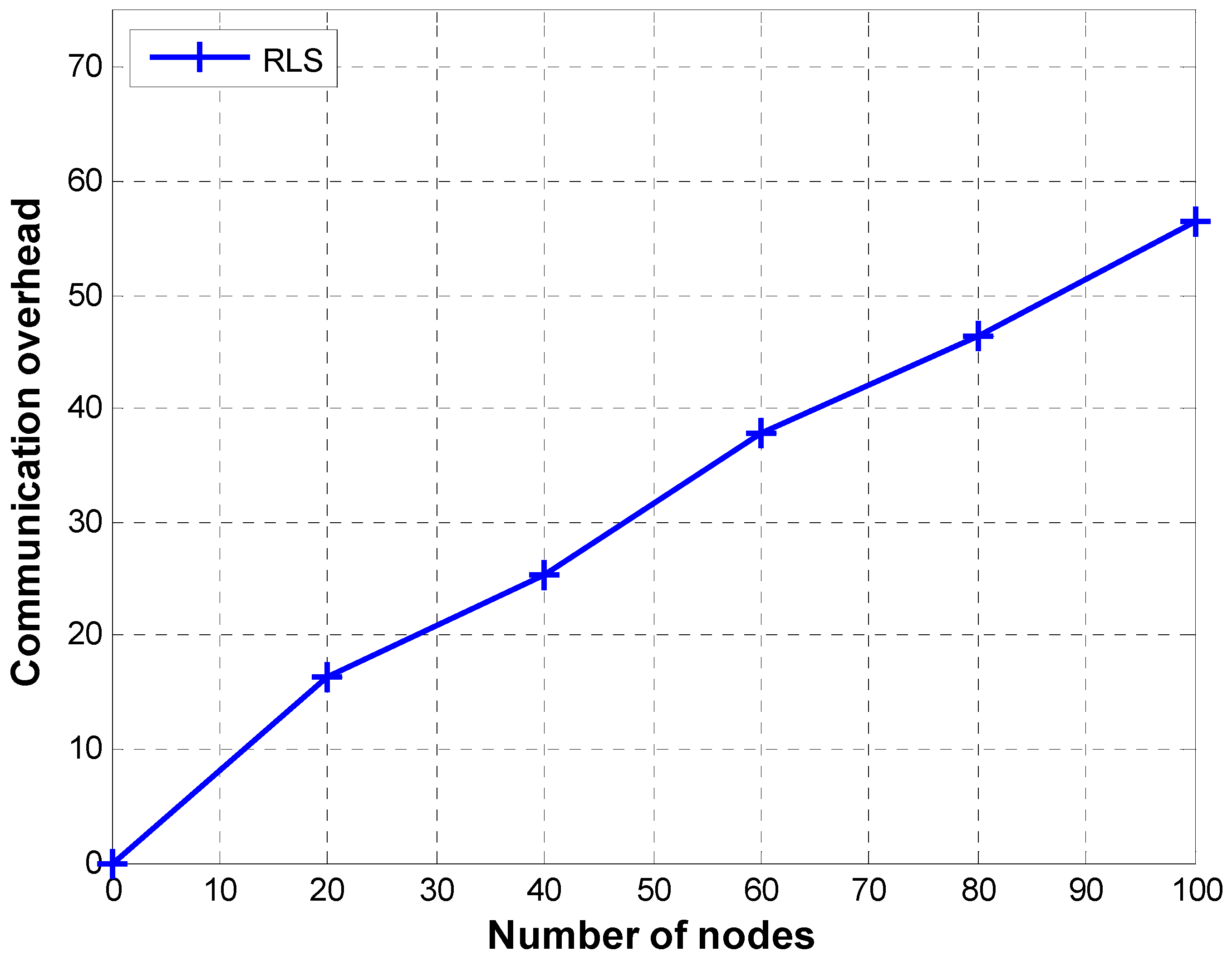
- Algorithm Stages: Localization schemes can be divided into two categories according to communication characteristics: (1) Single-stage schemes [30,31], and (2) multi-stage schemes [32,33,34]. In single-stage schemes, ordinary sensor nodes work in passive mode (i.e., they do not participate in localization activity except for activity related to their own localization). In case of single-stage protocol, ordinary sensor nodes do not act as reference nodes. Thus, they are not helpful for the localization of other ordinary nodes. However, in case of multi-stage protocols, an ordinary sensor node may act as a reference node as soon as it is localized. Unlocalized ordinary nodes can communicate with any of localized nodes to estimate their coordinates.The algorithm proposed in a previous study [35] is an example of a single-stage localization protocol. This algorithm uses a hyperbolic technique, normal distribution estimation error modeling, and calibration to localize a sensor node.The top-down positioning scheme proposed previously [36] is a multi-stage localization scheme. In this scheme, nodes are divided into three types: Anchor nodes that float on the water surface, reference nodes whose locations are known, and unlocalized nodes. Initially, as the localization process begins, nodes that fall within the range of anchor nodes are localized. Upon being localized, nodes can calculate confidence values and compare confidence values with confidence thresholds. If a node’s confidence value is higher than the confidence threshold, the node assumes the role of a reference node.TP-TSFLA [37] is another example of multi-stage localization schemes. It has 2-stages. Initially, during stage 1, reference nodes broadcast beacons. All those sensor nodes that receive beacons are localized using the received beacons. These newly localized nodes become reference nodes to help localize the remaining unlocalized node. In stage 2, all unlocalized nodes increase their transmission power to request beacon. Any localized node that receives the request responds with a beacon. The process of requesting localization beacon may continue until nodes are localized. This method may incur high communication overhead due to the fact that a particular unlocalized node may receive unnecessary beacons from a large number of reference nodes. Consequently, high communication overhead increases energy consumption.We will compare our technique with reverse localization scheme (RLS) [23]. The communication overhead incurred by RLS is shown in Figure 2. In case of RLS, for every node to be localized there are at least four transmissions, one by the sensor node and three by the surface reference nodes. Moreover, the number of transmissions increases if the signal transmitted by a sensor node is received by more than three reference nodes. The high communication overhead of RLS results in low bandwidth efficiency and high energy consumption.
3. Methodology
3.1. Protocol 1.1
Relative Localization Stage
Beacon Propagation
- It calculates its distance from the sender (node x) using RSSI and saves the calculated distance for future use.
- If the distance is more than the , node y adjusts its transmission power to yield a transmission range that is equal to the and retransmits B with appropriate header values as shown in Figure 5. (Guard value is used to compensate for variation in range due to channel impairments). Otherwise, node y retransmits B using default transmission power. B serves as ACK for the sender of the beacon (node x) and as a beacon for those nodes in node y’s range that did not receive a beacon from any other node. The “ACK-For” field in B contains ID of the node that should consider B as ACK (i.e., node x). Upon reception of ACK, node x calculates the position of node y relative to itself (i.e., node x) using TDoA.
- Calculate TWACK and go into wait state for the duration of TWACK. TWACK is the time period that a node that transmits a beacon will wait for ACKs in response to the beacon (B) is transmitted.
Backward Propagation of TRLs
Multi-Hop Relative Localization
Waiting Period
Handling Network Partitions
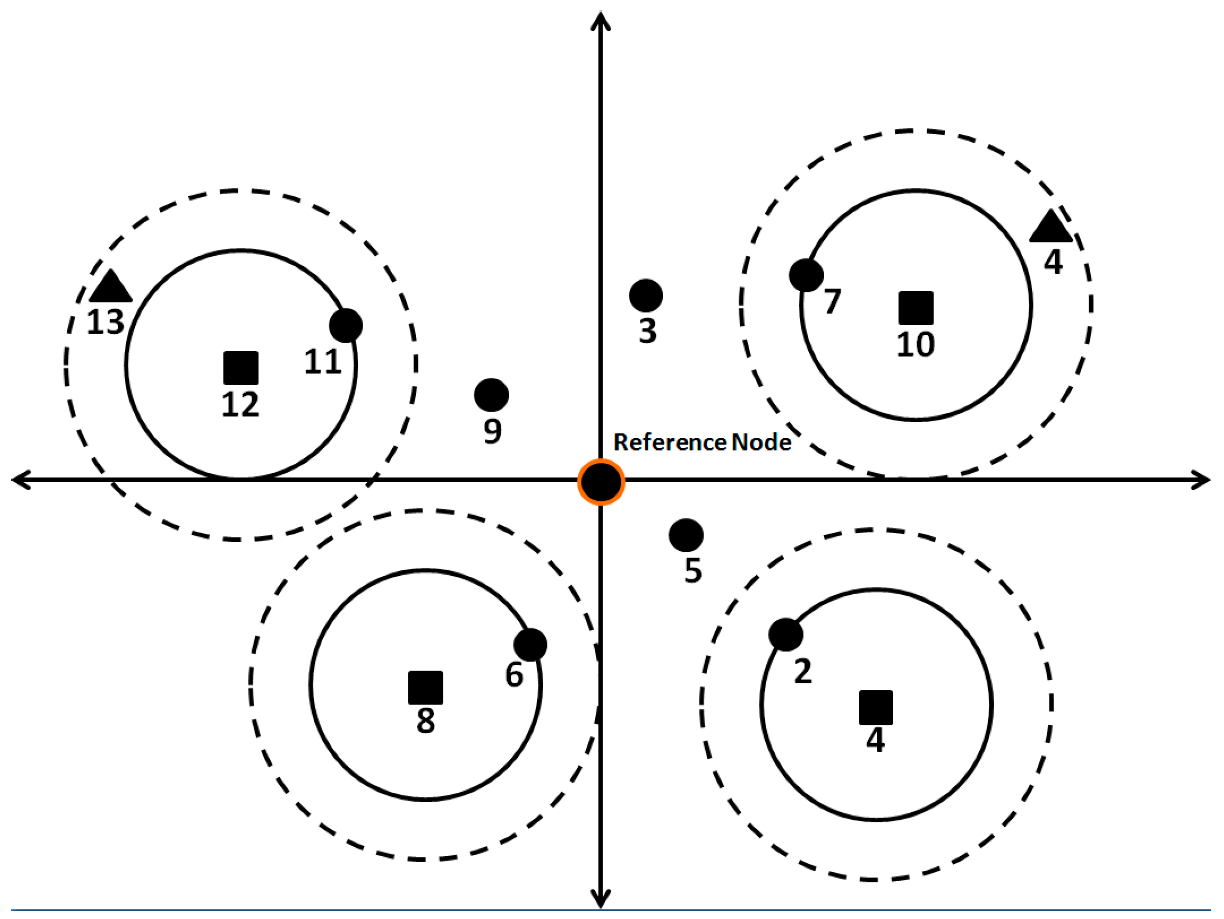
- The missing nodes can be in any direction relative to the reference node.
- The reference node can be located anywhere in the localized part of the network. For instance, it can be located somewhere in the center or in any direction far away from the center of the localized part of the network. If the GPS-enabled node is somewhere near the center, it will have to increase its range much more as compared to a node on the border of the localized part of the network in order to reach a missing node. If it is located far from the center in any particular direction and the missing nodes are located in the opposite direction, the reference node will have to increase its range even more compared to the case when it is situated in the center, thus wasting a lot of energy. Therefore, in order to save energy, we choose one farthest node in each quadrant. This ensures that unlocalized nodes are accessed with a much smaller increase in range, thus saving energy. Moreover, as the task is divided, the energy dissipation is fair. To make it fair, if a node has been used once to locate missing nodes, it will not be used again (for a certain number of times) even if it is the farthest in a quadrant. In such a case, the second farthest node will be used to locate missing nodes.
3.2. Protocol 1.2
3.3. Stage 2: Absolute Localization
3.3.1. Latitude Calculation:
- Node A is located in the southern hemisphere and node B is located south of node A or Node A is located in the northern hemisphere and node B is located north of node A. In this case, the latitude of B can be calculated using Equations (5) and (6).whereasLatB = distYAB° + LatAdistYAB° = DYAB(TRL)/111.2;DYAB(TRL) is obtained from Node A’s TRL. It is the distance between points A and B along Y axis in kilometers. In this case direction in LatB remains the same as the direction of LatA, i.e., both the points are located in the same hemisphere.Example:Node A’s absolute position = 20° S 150° ENode B is located 1668 KM to the South of A.distYAB° = 1668/111.2 = 15°LatB = 15° + 20° = 35° S
- Node A is located in the southern hemisphere and node B is located north of node A or Node A is located in the northern hemisphere and node B is located south of node A. whereas the distance (in degrees) between point A and B along latitude (i.e., distYAB°) is less than LatA. In this case, the latitude of B can be calculated using Equation (7).LatB = LatA − distYAB°In this case, the direction of LatB remains the same as the direction of LatA, i.e., both the points are located in the same hemisphere.Example:Node A’s absolute position = 20° S 150° ENode B is located 1668 KM to the North of A.distYAB° = 1668/111.2 = 15LatB = 20 − 15 = 5° S
- Node A is located in the southern hemisphere and node B is located north of node A or Node A is located in the northern hemisphere and node B is located south of node A. Whereas the distance (in degrees) between point A and B along latitude (i.e., distYAB°) is greater than LatA. In this case the latitude of B can be calculated using Equation (8).LatB = distYAB° − LatAIt is important to mention that in this case direction in LatB is opposite of A, e.g., if LatA is in the south then LatB is in the north.ExampleNode A’s absolute position = 10° S 150° EB is located 1668 KM to the North of A at 150° EdistYAB° = 1668/111.2 = 15LatB = 15 − 10 = 5° N
3.3.2. Longitude Calculation:
- Node A is located in eastern hemisphere and node B is located east of node A or Node A is located in western hemisphere and node B is located west of node A. In this case the longitude of B can be calculated using Equations (9) and (10).whereasLongB = distXAB° + LongAdistXAB° = DXAB(TRL)/(111.2 × cos(lat(A)));In this case, the direction of LongB remains the same as the direction of longA, i.e., if LongA is east then Long B is also east or if LongA is west, then LongB is also west.Example:Node A’s absolute position = 20° S 50° EB is located 2403.36 KM to the East of A at 20° SdistXAB° = 2403.36/(111.2 × cos(20)) ≈ 23°;LongB = 23° + 50°= 73° E
- Node A is located in Eastern hemisphere and Node B is located west of Node A or Node A is located in western hemisphere and node B is located east of node A. Whereas the distance (in degrees) between point A and B along longitude (i.e., distXAB°) is less than LongA. In this case the longitude of B can be calculated using Equation (11).LongB = LongA − distXAB°In this case, the direction of LatB remains the same as the direction of LatA, i.e., both the points are located in the same hemisphere.Example:Node A’s absolute position = 20° S 50° EB is located 2403.36 KM to the west of A at 20° SdistXAB° = 2403.36/(111.2 × cos(20)) ≈ 23°;LongB = 50° − 23°= 27° E
- Node A is located in Eastern hemisphere and Node B is located west of Node A or Node A is located in western hemisphere and node B is located east of node A. Whereas the distance (in degrees) between point A and B along longitude (i.e., distXAB°) is greater than LongA. In this case, the longitude of B can be calculated using Equation (12).LongB = distXAB° − LongAIts important to mention that in this case direction in LongB is opposite of A, e.g., if LongA is east, then LongB is westExample:Node A’s absolute position = 20° S 10° EB is located 2403.36 KM to the west of A at 20° SdistXAB° = 2403.36/(111.2 × cos(20)) ≈ 23°;LongB = 23° − 10°= 13° W
4. Simulation Setup
4.1. Underwater Energy Consumption Model
4.2. Parameters Setting
5. Results and Discussion
5.1. Fixed Simulation Area
5.1.1. Communication Overhead
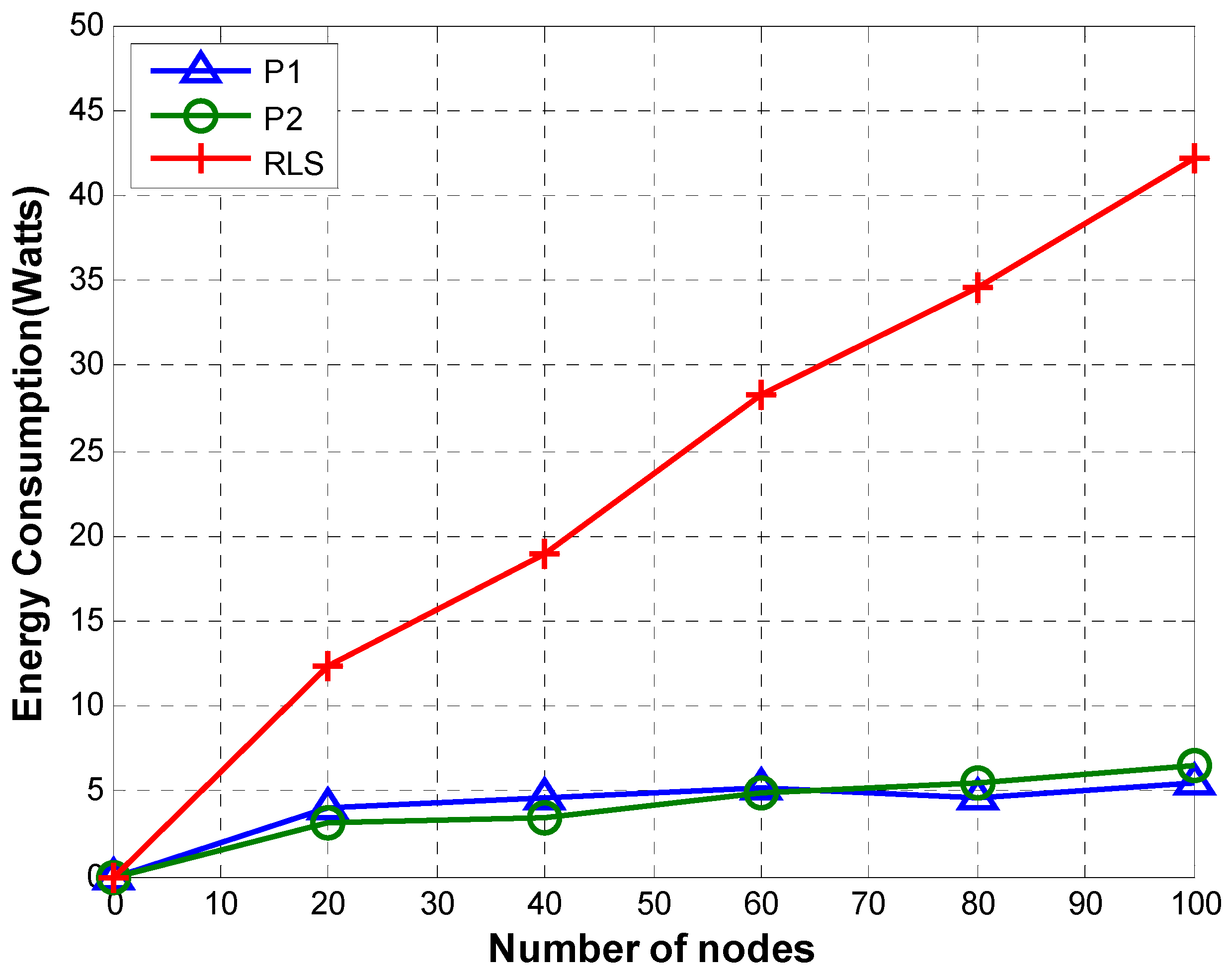
5.1.2. Energy Consumption
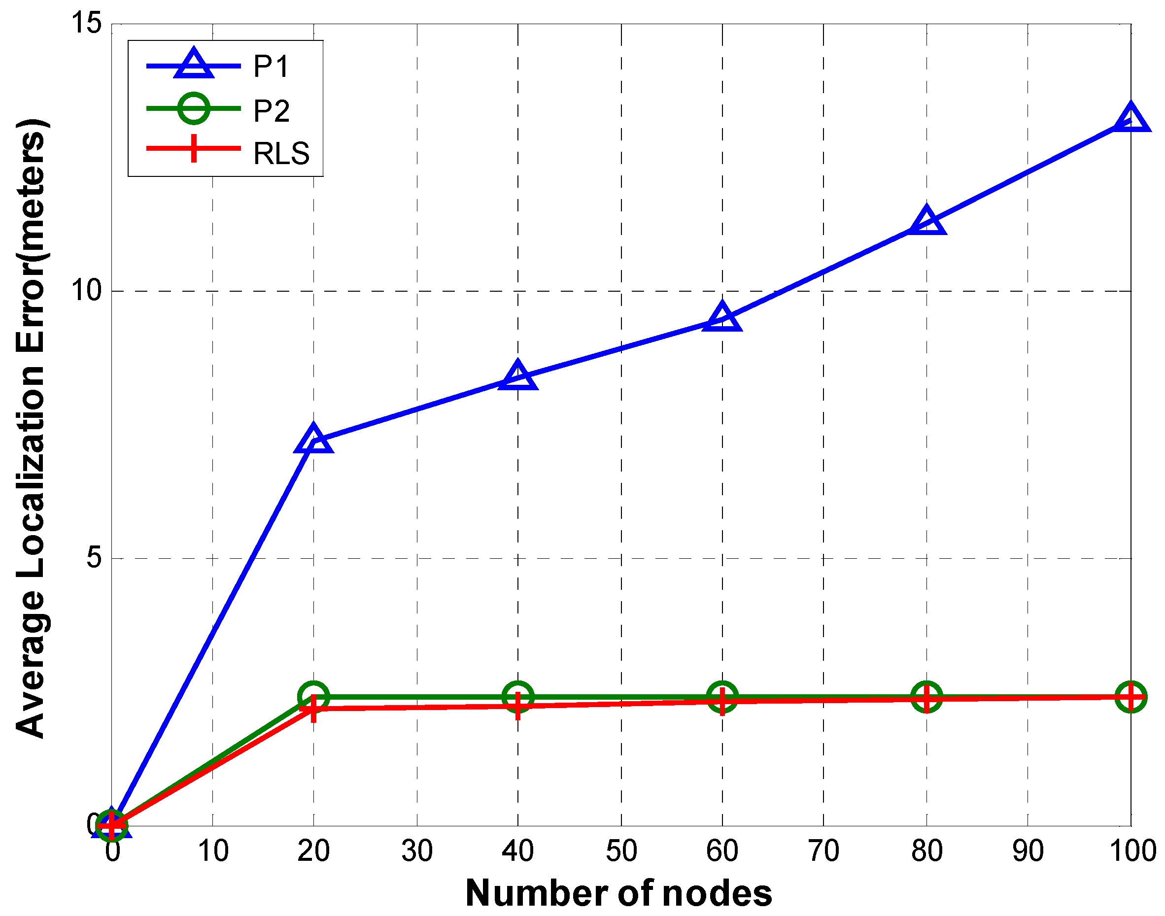
5.1.3. Localization Error
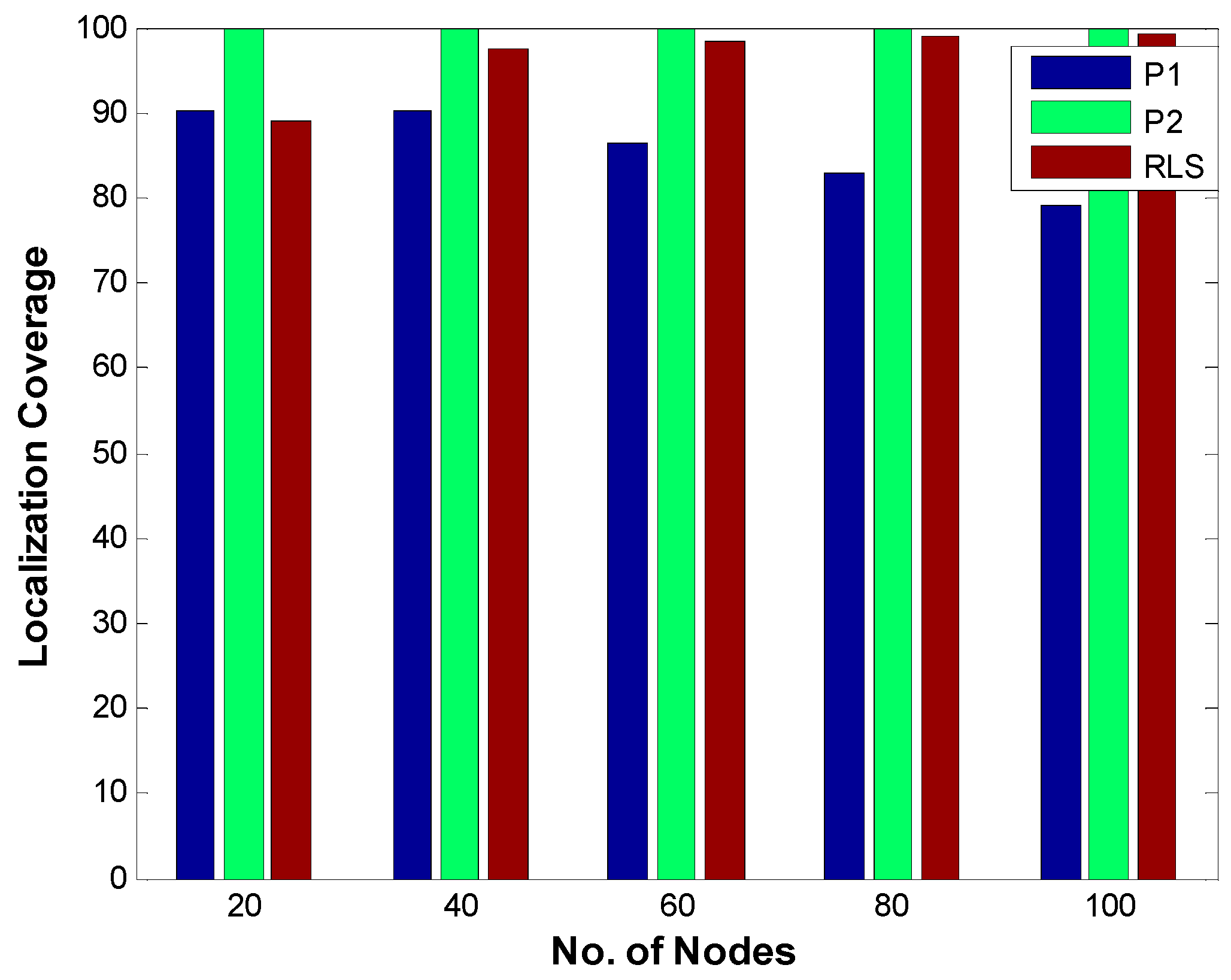
5.1.4. Localization Coverage
5.2. Sparsity
5.2.1. Communication Overhead
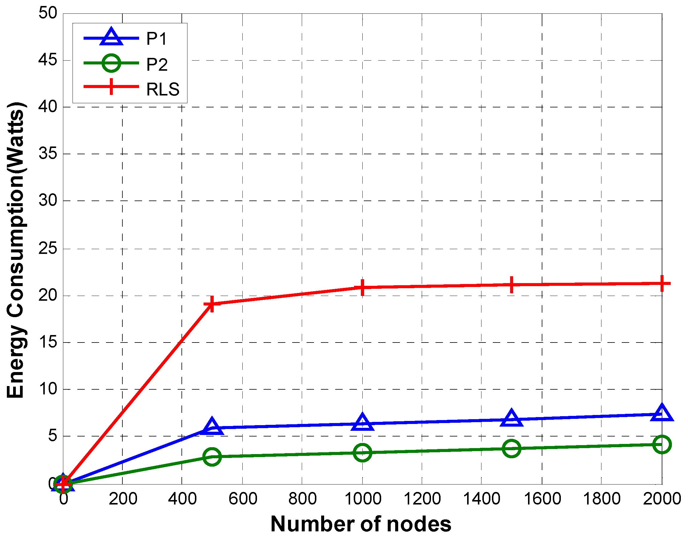
5.2.2. Energy Consumption
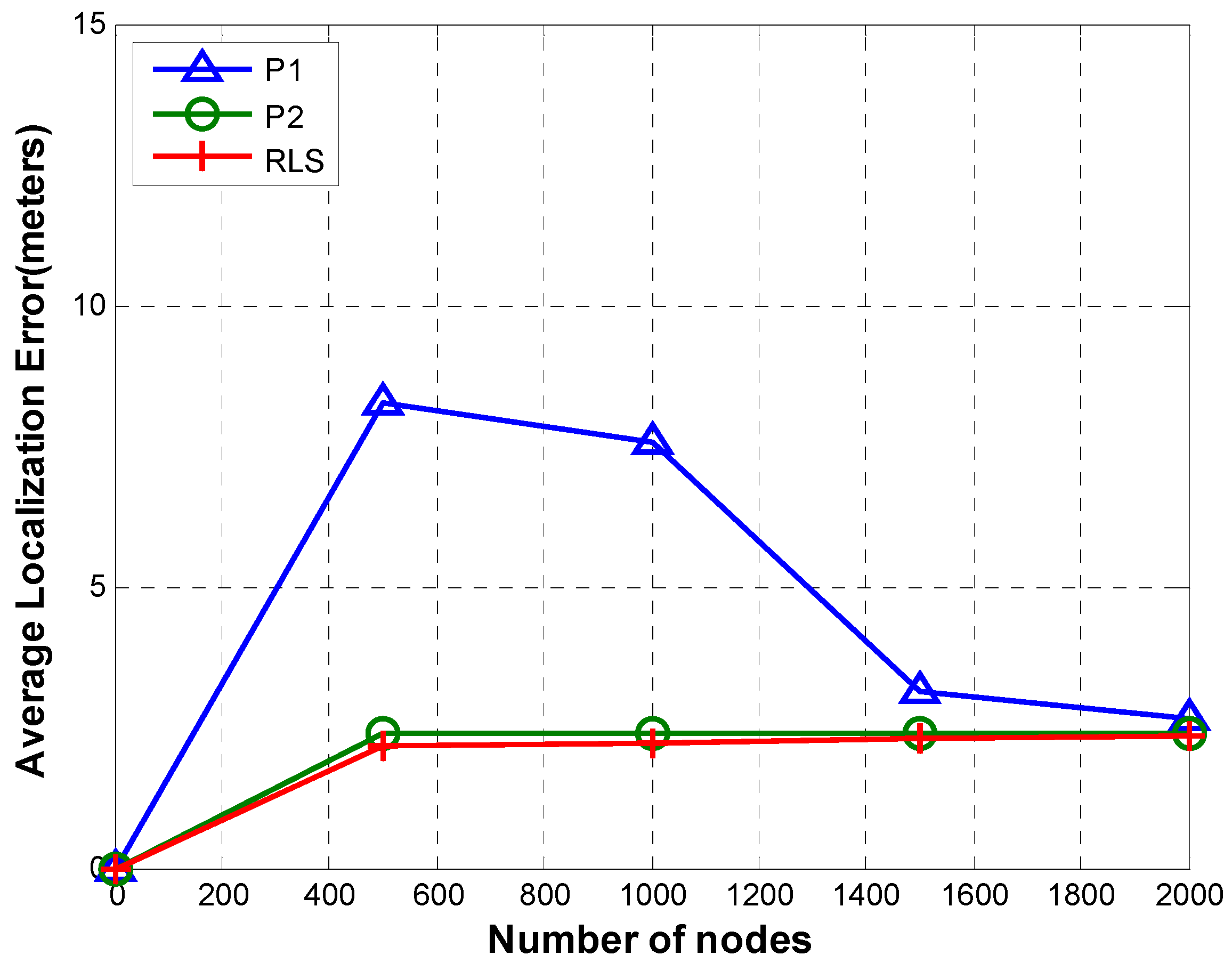
5.2.3. Localization Error
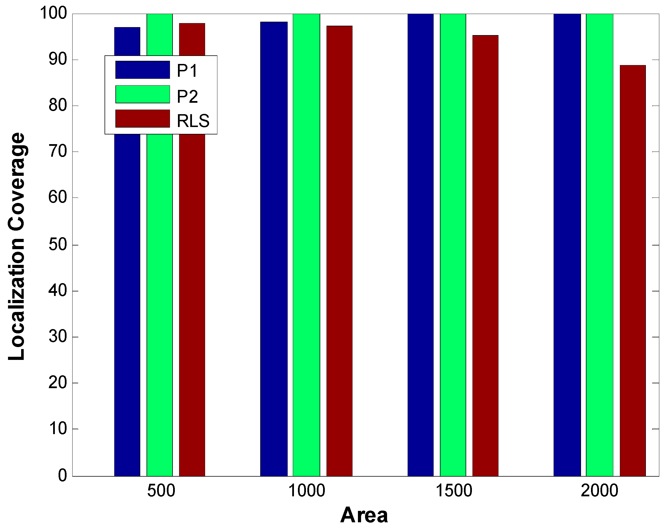
5.2.4. Localization Coverage
6. Conclusions
Author Contributions
Funding
Conflicts of Interest
References
- Dehnavi, M.S.; Ayati, M.; Zakerzadeh, M.R. Three dimensional target tracking via Underwater Acoustic Wireless Sensor Network. In Proceedings of the Artificial Intelligence and Robotics (IRANOPEN), Qazvin, Iran, 9 April 2017. [Google Scholar]
- Xie, P.; Kang, F.; Wang, S. Research for underwater target tracking by using multi-sonar. In Proceedings of the 2010 3rd International Congress on Image and Signal Processing (CISP), Yantai, China, 16–18 October 2010; Volume 9. [Google Scholar]
- Coleman, D.F.; Ballard, R.D.; Gregory, T. Marine archaeological exploration of the Black Sea. In Proceedings of the Oceans 2003. Celebrating the Past … Teaming Toward the Future, San Diego, CA, USA, 22–26 September 2003; Volume 3. [Google Scholar]
- Levin, D.; Seidel, J.; Gosman, M.; Trembanis, A.; Drutjons, M.; Buskop, J.; Culp, J. A convenient testbed for applying marine technology to shipwreck investigations and a tool for contagious STEM focused education in marine exploration and research. In Proceedings of the 2013 Oceans-San Diego, San Diego, CA, USA, 23–27 September 2013. [Google Scholar]
- Rosen, D.; Lauermann, A. It’s all about your network: Using ROVs to assess Marine Protected Area effectiveness. In Proceedings of the OCEANS 2016 MTS/IEEE Monterey, Monterey, CA, USA, 19–23 September 2016. [Google Scholar]
- Tchertchian, N.; Millet, D. Eco-maintenance for complex systems: Application on system of renewable energy production. In Proceedings of the 2014 3rd International Symposium on Environmental Friendly Energies and Applications (EFEA), St. Ouen, France, 19–21 November 2014. [Google Scholar]
- Luo, J.; Fan, L.; Wu, S.; Yan, X. Research on localization algorithms based on acoustic communication for underwater sensor networks. Sensors 2018, 18, 67. [Google Scholar] [CrossRef]
- Kumar, R. A survey on data aggregation and clustering schemes in underwater sensor networks. Int. J. Grid Distrib. Comput. 2014, 7, 29–52. [Google Scholar] [CrossRef]
- Kim, K.-Y.; Shin, Y. A distance boundary with virtual nodes for the weighted centroid localization algorithm. Sensors 2018, 18, 1054. [Google Scholar] [CrossRef] [PubMed]
- Liu, P.; Zhang, X.; Tian, S.; Zhao, Z.; Sun, P. A novel virtual anchor node-based localization algorithm for wireless sensor networks. In Proceedings of the Sixth International Conference on Networking (ICN’07), Martinique, France, 22–28 April 2007; p. 9. [Google Scholar]
- Felemban, E.; Shaikh, F.K.; Qureshi, U.M.; Sheikh, A.A.; Qaisar, S.B. Underwater sensor network applications: A comprehensive survey. Int. J. Distrib. Sens. Netw. 2015, 11, 896832. [Google Scholar] [CrossRef]
- Heidemann, J.; Ye, W.; Wills, J.; Syed, A.; Li, Y. Research challenges and applications for underwater sensor networking. In Proceedings of the Wireless Communications and Networking Conference 2006, Las Vegas, NV, USA, 3–6 April 2006; Volume 1. [Google Scholar]
- Akyildiz, I.F.; Pompili, D.; Melodia, T. Underwater acoustic sensor networks: Research challenges. Ad Hoc Netw. 2005, 3, 257–279. [Google Scholar] [CrossRef]
- Xie, P.; Zhou, Z.; Nicolaou, N.; See, A.; Cui, J.-H.; Shi, Z. Efficient vector-based forwarding for underwater sensor networks. EURASIP J. Wirel. Commun. Netw. 2010, 2010, 195910. [Google Scholar] [CrossRef] [PubMed]
- Nicolaou, N.; See, A.; Xie, P.; Cui, J.-H.; Maggiorini, D. Improving the robustness of location-based routing for underwater sensor networks. In Proceedings of the Oceans 2007—Europe 18, Aberdeen, UK, 18–21 June 2007. [Google Scholar]
- Anupama, K.R.; Sasidharan, A.; Vadlamani, S. A location-based clustering algorithm for data gathering in 3D underwater wireless sensor networks. In Proceedings of the 2008 International Symposium on Telecommunications, Tehran, Iran, 27–28 August 2008; pp. 343–348. [Google Scholar]
- Tan, H.P.; Diamant, R.; Seah, W.K.; Waldmeyer, M. A survey of techniques and challenges in underwater localization. Ocean Eng. 2011, 38, 1663–1676. [Google Scholar] [CrossRef]
- Urick, R.J. Principles of Underwater Sound for Engineers, 3rd ed.; (Reprinted 1996, Peninsula Publ., Los Altos, CA); McGraw-Hill: New York, NY, USA, 1983; 423p. [Google Scholar]
- Shin, D.-H.; Sung, T.-K. Comparisons of error characteristics between TOA and TDOA positioning. IEEE Trans. Aerosp. Electron. Syst. 2002, 38, 307–311. [Google Scholar] [CrossRef]
- Compensation of Multipath Fading in Underwater Spread-Spectrum Communication Systems. Available online: https://ieeexplore.ieee.org/stamp/stamp.jsp?tp=&arnumber=670153 (accessed on 29 March 2019).
- Erol-Kantarci, M.; Mouftah, H.T.; Oktug, S. A survey of architectures and localization techniques for underwater acoustic sensor networks. IEEE Commun. Surv. Tutor. 2011, 13, 487–502. [Google Scholar] [CrossRef]
- Tsai, P.-H.; Tsai, R.-G.; Wang, S.-S. Hybrid Localization Approach for Underwater Sensor Networks. J. Sens. 2017, 2017, 5768651. [Google Scholar] [CrossRef]
- Moradi, M.; Rezazadeh, J.; Ismail, A.S. A reverse localization scheme for underwater acoustic sensor networks. Sensors 2012, 12, 4352–4380. [Google Scholar] [CrossRef]
- Chandrasekhar, V.; Seah, W. An area localization scheme for underwater sensor networks. In Proceedings of the OCEANS 2006—Asia Pacific, Singapore, 16–19 May 2007; pp. 1–8. [Google Scholar]
- Liu, L.; Wu, J.; Zhu, Z. Multihops fitting approach for node localization in underwater wireless sensor networks. Int. J. Distrib. Sens. Netw. 2015, 11, 682182. [Google Scholar] [CrossRef]
- Cheng, X.; Shu, H.; Liang, Q.; Du DH, C. Silent positioning in underwater acoustic sensor networks. IEEE Trans. Veh. Technol. 2008, 57, 1756–1766. [Google Scholar] [CrossRef]
- Luo, H.; Guo, Z.; Dong, W.; Hong, F.; Zhao, Y. LDB: Localization with directional beacons for sparse 3D underwater acoustic sensor networks. J. Netw. 2010, 5. [Google Scholar] [CrossRef]
- Luo, H.; Zhao, Y.; Guo, Z.; Liu, S.; Chen, P.; Ni, L.M. UDB: Using directional beacons for localization in underwater sensor networks. In Proceedings of the 2008 14th IEEE International Conference on Parallel and Distributed Systems, Melbourne, Australia, 8–10 December 2008. [Google Scholar]
- Islam, T.; Lee, Y.K. A Cluster Based Localization Scheme with Partition Handling for Mobile Underwater Acoustic Sensor Networks. Sensors 2019, 19, 1039. [Google Scholar] [CrossRef]
- Bhuvaneswari PT, V.; Karthikeyan, S.; Jeeva, B.; Prasath, M.A. An efficient mobility based localization in underwater sensor networks. In Proceedings of the 2012 Fourth International Conference on Computational Intelligence and Communication Networks, Mathura, India, 3–5 November 2012. [Google Scholar]
- Diamant, R.; Lampe, L. Underwater localization with time-synchronization and propagation speed uncertainties. IEEE Trans. Mob. Comput. 2013, 12, 1257–1269. [Google Scholar] [CrossRef]
- Zhou, Z.; Peng, Z.; Cui, J.H.; Shi, Z.; Bagtzoglou, A. Scalable localization with mobility prediction for underwater sensor networks. IEEE Trans. Mob. Comput. 2011, 10, 335–348. [Google Scholar] [CrossRef]
- Kurniawan, A.; Ferng, H.-W. Projection-based localization for underwater sensor networks with consideration of layers. In Proceedings of the TENCON Spring Conference 2013, Sydney, Australia, 17–19 April 2013. [Google Scholar]
- Ren, Y.; Yu, N.; Guo, X.; Wan, J. Cube-scan-based three dimensional localization for large-scale underwater wireless sensor networks. In Proceedings of the 2012 IEEE International Systems Conference SysCon 2012, Vancouver, BC, Canada, 19–22 March 2012. [Google Scholar]
- Bian, T.; Venkatesan, R.; Li, C. Design and evaluation of a new localization scheme for underwater acoustic sensor networks. In Proceedings of the GLOBECOM 2009—2009 IEEE Global Telecommunications Conference, Honolulu, HI, USA, 30 November–4 December 2009. [Google Scholar]
- Zhang, S.; Zhang, Q.; Liu, M.; Fan, Z. A top-down positioning scheme for underwater wireless sensor networks. Sci. China Inf. Sci. 2014, 57, 1–10. [Google Scholar] [CrossRef]
- Luo, J.; Fan, L. A Two-Phase time synchronization-free localization algorithm for underwater sensor networks. Sensors 2017, 17, 726. [Google Scholar] [CrossRef]
- World Maps. Available online: https://wiki--travel.com/detail/world-map-with-latitude-and-longitude-coordinates-3.html (accessed on 29 March 2019).
- Stojanovic, M. On the relationship between capacity and distance in an underwater acoustic communication channel. ACM SIGMOBILE Mob. Comput. Commun. Rev. 2007, 11, 34–43. [Google Scholar] [CrossRef]
- Gao, J.L. Analysis of energy consumption for ad hoc wireless sensor networks using a bit-meter-per-joule metric. IPN Prog. Rep. 2002, 42, 1–19. [Google Scholar]
- Evo Logics. Available online: http://www.evologics.de/en/products/acoustics/s2cr_48_78.html (accessed on 7 March 2019).


| Node Type/Ack Status. | One or More ACKs Received | No ACKs Received |
|---|---|---|
| Reference node | 1. Calculate the relative position of the sender using TDoA. 2. At the end of TWACK, compare reference node’s TRL with the list of all nodes. If the two lists match, it means all nodes have been localized relative to the reference node. Therefore, it sends TRL to C&C. However, if the two lists do not match, then it sets TWTRL1 (i.e., waiting time to receive TRLs of nodes of tier 1). | It means that none of the nodes is within the default range of the reference node. Therefore, it calls partition handling routine. (explained at the end of Section 3.1) |
| Any ordinary node x | 1. Calculate the relative position of the sender (i.e., the node that sent ACK). 2. At the end of TWACK, node x sends its TRL to the upstream node from which it received a beacon. 3. Node x sets TWTRL1 (i.e., waiting time for TRL(s) from the next tier down the stream). | No Action |
| Node Type/TRL Reception Status | One or More TRLs Received | No TRLs Received |
|---|---|---|
| Reference node | 1. Apply lemma 2 to calculate relative positions of the newly introduced nodes (i.e., nodes in the received TRL) using: a. The relative position information in received TRL(s) b. The relative position (w.r.t. the reference node) of the node that owns the TRL. 2. At the end of TWTRL, the reference node compares its TRL with the list of all nodes. If the two lists match, it means all nodes have been localized relative to the reference node. Therefore, no further action is required. However, if the two lists do not match, then the reference node sets next TWTRL (i.e., waiting time to receive TRLs of nodes of the next tier). | It means that some nodes cannot be accessed with current transmission power. Therefore, the reference node calls partition handling routine which involves increasing the transmission power of certain nodes. |
| Any ordinary node x | 1. At the end of TWTRL, node x sends the TRL received from a downstream node to the upstream node from which it received a beacon. 2. Sets next TWTRL i.e., waiting time for TRL’s from tiers further down the stream | No Action |
| Time/Nodes | Node 1 | Node 2 | Node 3 | Node 4 |
|---|---|---|---|---|
| 0 | Node 1 transmits beacon Sets TWACK = 2Pd | |||
| Pd | TWACK = Pd | B(beacon) arrives at node 2 Node 2 sets it TWACK = 2Pd Transmits B | ||
| 2xPd | 2’s B(Ack) reaches node 1 Node 1 calculate the relative position of node 2 All nodes localized = false Sets TWTRL1 = 2Pd | Node 2’s TWACK = Pd | Node 2’s B(beacon) arrives at node 3 Node 3 sets it TWACK = 2Pd Transmits B | |
| 3xPd | TWTRL1 = Pd | Node 3’s B(Ack) arrives at node 2 TWACK = 0 2 calculates relative position of 3 Sends TRL to 1 2 sets TWTRL1 = 2Pd | TWACK = Pd | Node 3’s B(beacon) arrives at node 4 Node 4 sets TWACK = 2Pd Transmits B |
| 4xPd | 2’s TRL arrives at 1 1 calculates relative positions of node 3 using Lemma 1 TWTRL1 = 0 All nodes localized = false 1 sets TWTRL2 = 2Pd | TWTRL1 = PD | 4’s B (Ack) arrives at 3. 3 calculates relative position of 4 TWACK = 0 3 sends TRL to 2 Sets TWTRL1 = 2Pd | TWACK = Pd |
| 5xPd | TWTRL2 = Pd | Received TRL from 3 TWTRL = 0 Send received TRL to 1 Set TWTRL2 = 2Pd | TWTRL1 = Pd | TWACK = 0 Nothing Received No Action |
| 6xPd | TWTRL2 = 0 3’s TRL arrives at 1 1 calculates the relative position of 4 using lemma 1 All nodes localized = True Send TRL of node 1 to the surface GPS node | TWTRL2 = Pd | TWTRL1 = 0 Nothing Received No Action | No Action |
| 7Pd | No Action | TWTRL2 = 0 Nothing Received No Action | No Action | No Action |
| Parameters | Values |
|---|---|
| Area | 500 × 500, 1000 × 1000, 1500 × 1500, 2000 × 2000 |
| Default Range | 250 |
| No. of nodes | 20, 40, 60, 80, 100 |
| No. of partitions | 1, 2, 3, 4 |
| Packet Size | 512 bits |
| Data rate | 5000 bps |
| Error in propagation speed | 0.2 m/s [23] |
| Error in depth measurement | 0.1 m [23] |
| Mobility based error | 0.1 m |
| Simulation Runs | 100 |
| Energy Consumption | Range |
|---|---|
| 5.5 W | 250 m |
| 8 W | 500 m |
| 18 W | 1000 m |
| 60 W | Above 1000 m |
© 2019 by the authors. Licensee MDPI, Basel, Switzerland. This article is an open access article distributed under the terms and conditions of the Creative Commons Attribution (CC BY) license (http://creativecommons.org/licenses/by/4.0/).
Share and Cite
Islam, T.; Lee, Y.K. A Two-Stage Localization Scheme with Partition Handling for Data Tagging in Underwater Acoustic Sensor Networks. Sensors 2019, 19, 2135. https://doi.org/10.3390/s19092135
Islam T, Lee YK. A Two-Stage Localization Scheme with Partition Handling for Data Tagging in Underwater Acoustic Sensor Networks. Sensors. 2019; 19(9):2135. https://doi.org/10.3390/s19092135
Chicago/Turabian StyleIslam, Tariq, and Yong Kyu Lee. 2019. "A Two-Stage Localization Scheme with Partition Handling for Data Tagging in Underwater Acoustic Sensor Networks" Sensors 19, no. 9: 2135. https://doi.org/10.3390/s19092135
APA StyleIslam, T., & Lee, Y. K. (2019). A Two-Stage Localization Scheme with Partition Handling for Data Tagging in Underwater Acoustic Sensor Networks. Sensors, 19(9), 2135. https://doi.org/10.3390/s19092135