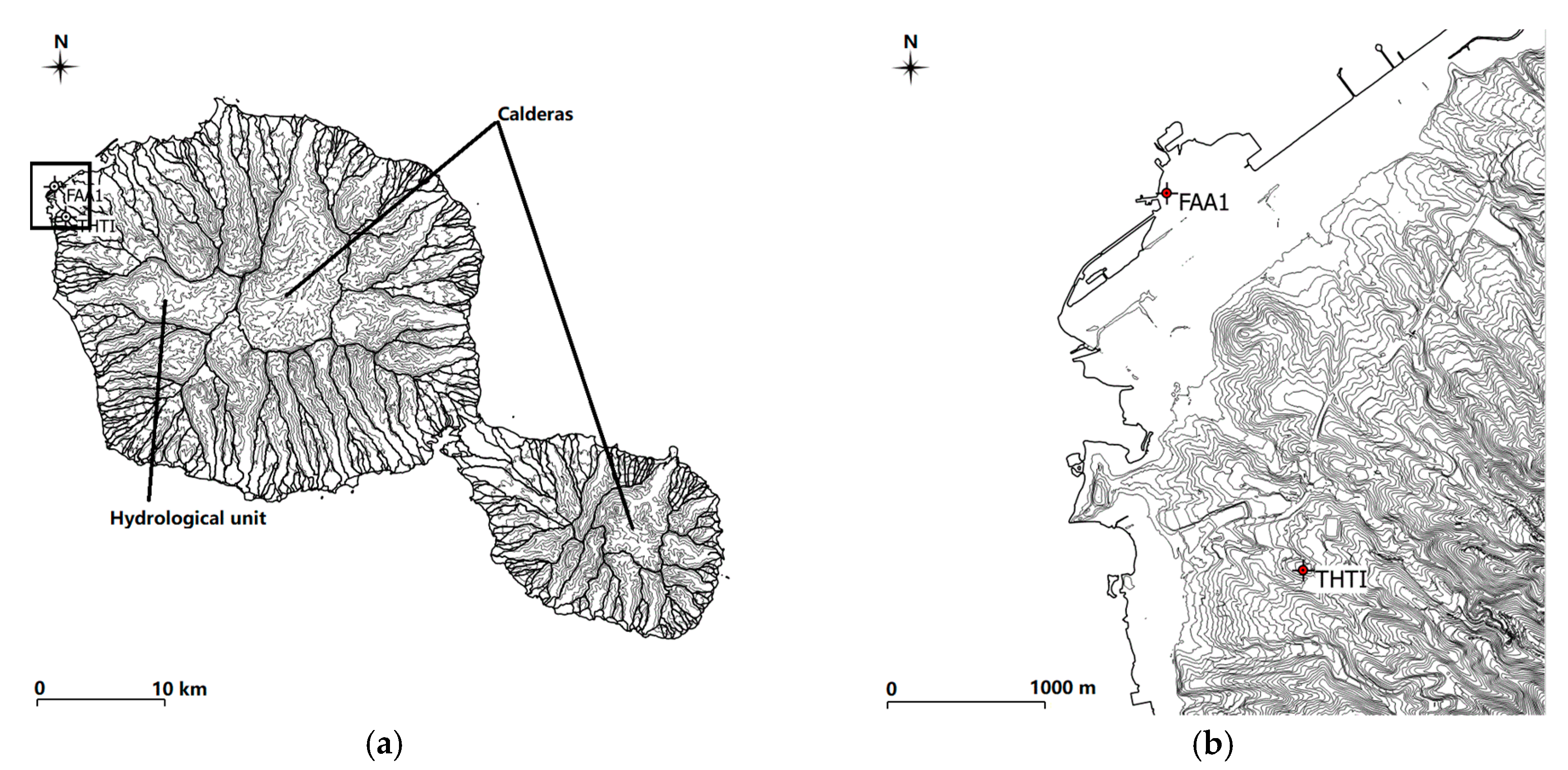
Figure 1.
Location of the two nearby GPS stations (THTI (149.61° W, 17.58° S, ellipsoidal altitude 98.49 m) and FAA1 (149.62° W, 17.56° S, ellipsoidal altitude 12.35 m) in the Tahiti Island. (a) Tahiti Nui shield volcano (30 km in diameter) and Tahiti Iti volcano (15 km diameter), joined by the isthmus of Taravao. Tahiti is located in the South Pacific, at mid-distance from South America to Australia. The contour lines of the topography are every 200 m, with the limits of hydrographic units, mostly radial valleys, indicated by bold lines. (b) Enlargement of (a), near the two stations, with contour lines of the topography every 5 m. The airstrip is clearly visible on the enlargement, close to the FAA1 station. The calderas (volcano pits) are indicated in the figures as well as hydrological units (watersheds).
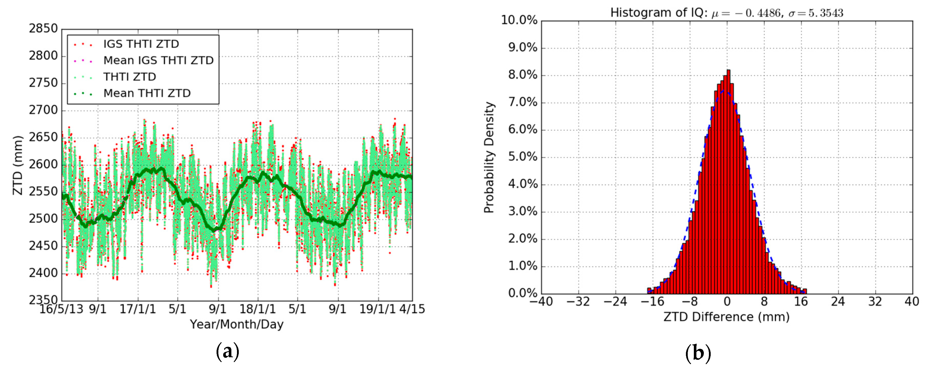
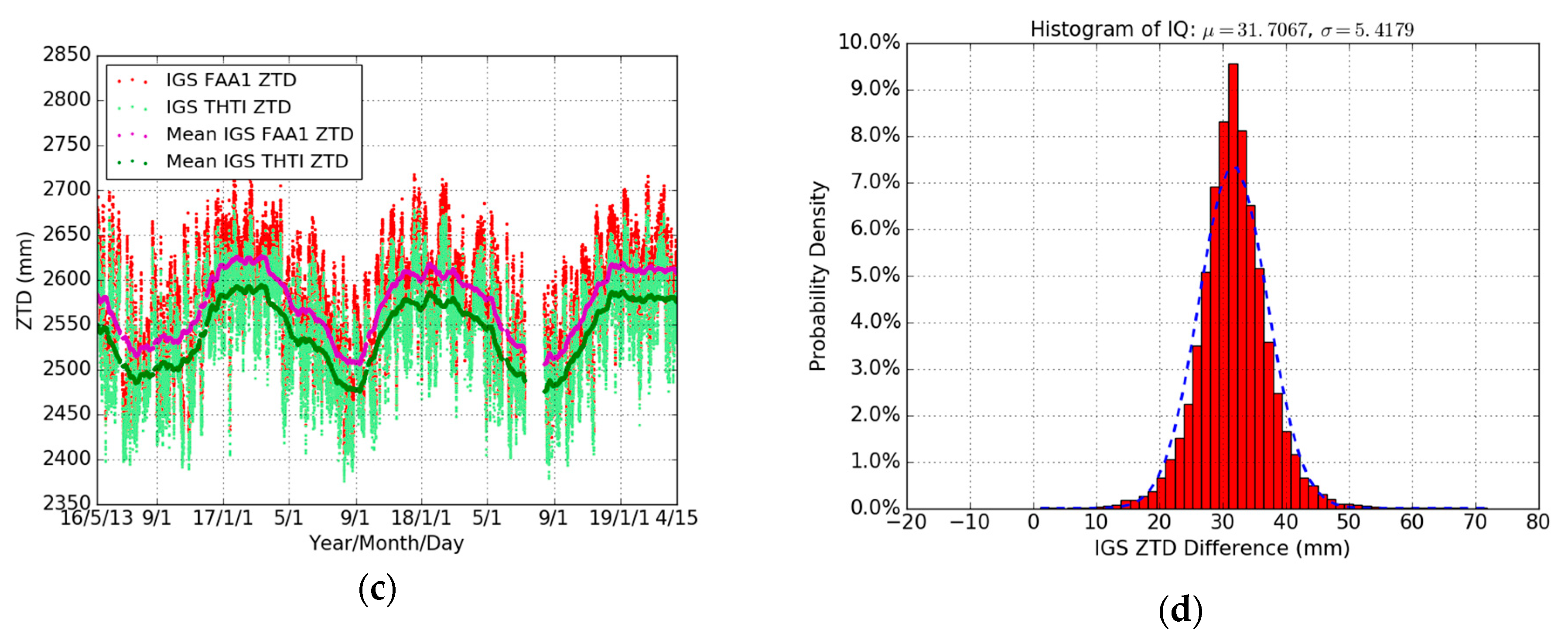
Figure 2.
Comparisons of our THTI ZTD values (light-green dots) with IGS THTI ZTD (red dots), and monthly averaged estimates of our THTI ZTD (green dots) and IGS THTI ZTD (magenta dots) (a) and our FAA1 ZTD (light-green dots) with IGS FAA1 ZTD (red dots)), and monthly averaged estimates of our FAA1 ZTD (green dots) and IGS FAA1 ZTD (magenta dots) (c), and the histograms of IQ (intelligence quotient) for the corresponding ZTD differences between GPS THTI ZTD and IGS THTI ZTD (b) and between GPS FAA1 ZTD and IGS FAA1 ZTD (d).
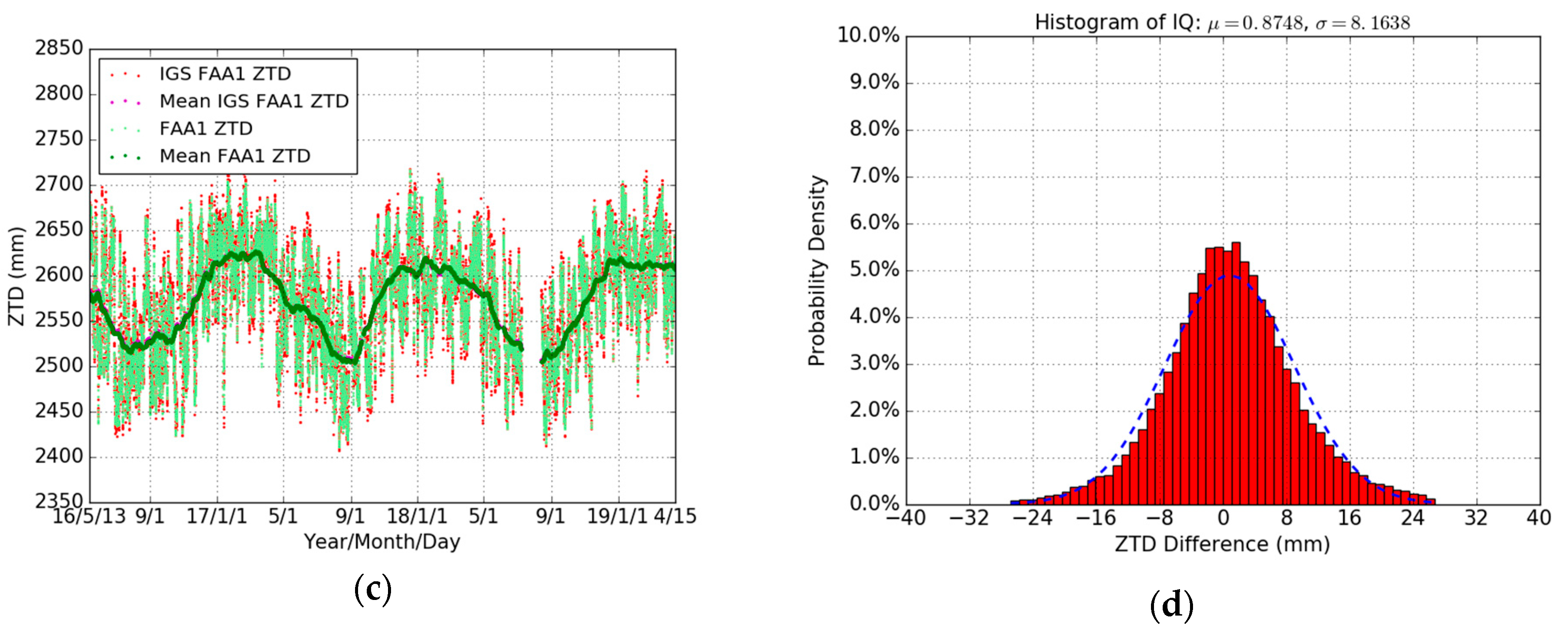
Figure 3.
Comparisons between our THTI ZTD estimates (light-green dots) and our FAA1 ZTD estimates (red dots), and monthly averaged estimates of the THTI ZTD (green dots) and FAA1 ZTD (magenta dots) (a), and IGS THTI ZTD estimates (light-green dots) versus IGS FAA1 ZTD estimates (red dots), and monthly averaged estimates of the IGS THTI ZTD (green dots) and IGS FAA1 ZTD (magenta dots) (c), and the corresponding ZTD differences between THTI ZTDs and FAA1 ZTDs (b) and between IGS THTI ZTDs and IGS FAA1 ZTDs (d).
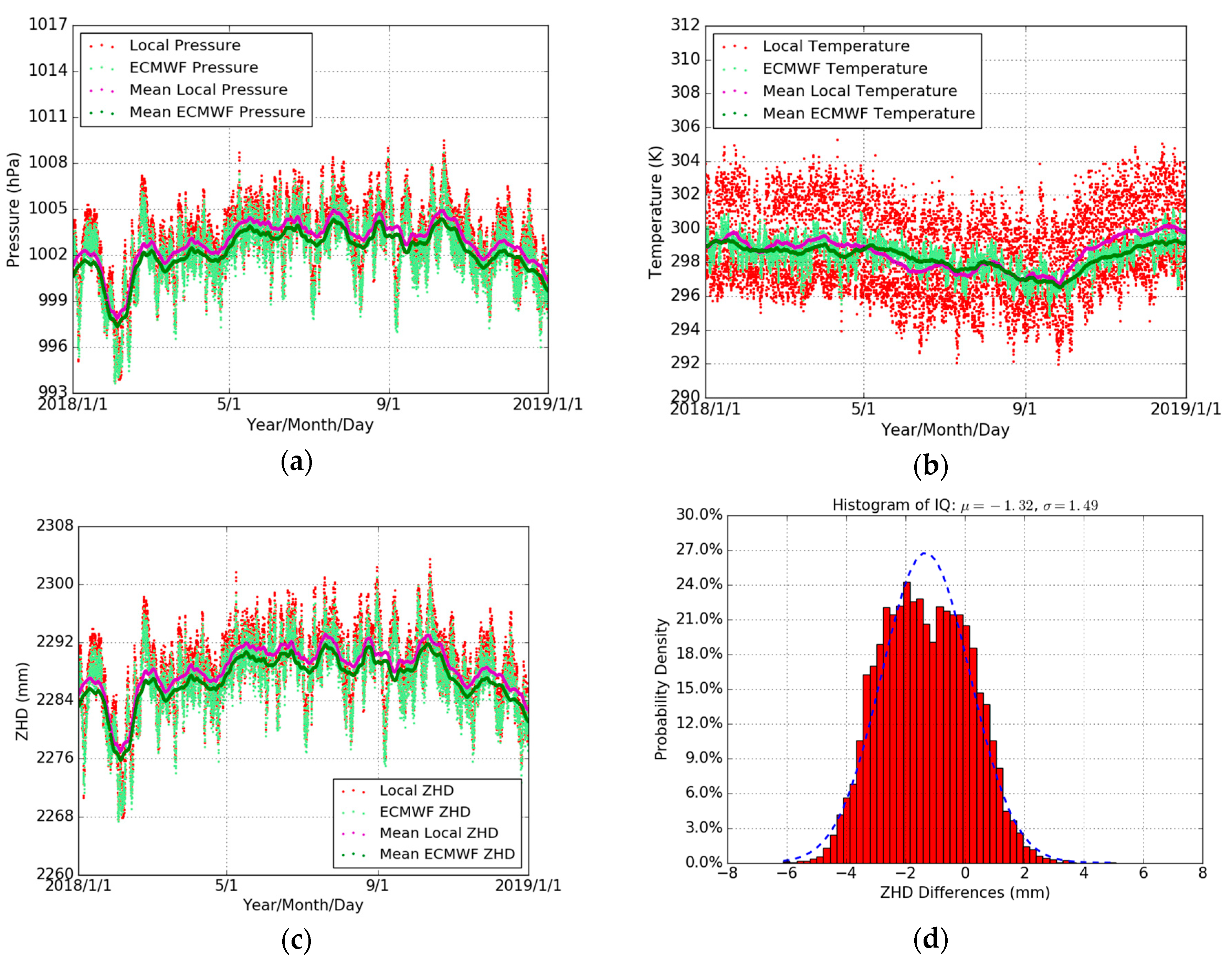
Figure 4.
Comparisons of ECMWF pressure (light-green dots) with local pressure (red dots), and 10 days averaged estimates of the ECMWF pressure (green dots) and local pressure (magenta dots) (a), and ECMWF temperature (light-green dots) with local temperature (red dots), and 10 days averaged estimates of the ECMWF temperature (green dots) and local temperature (magenta dots) (b), and the time series of ZHD derived from ECMWF pressure (light green dots) and local pressure (red dots), and every 10 days averaged estimates of the ECMWF ZHD (green dots) and local ZHD (magenta dots) (c), and the histogram of ZHD difference (d) during the whole year of 2018. The temporal resolution is one hour.
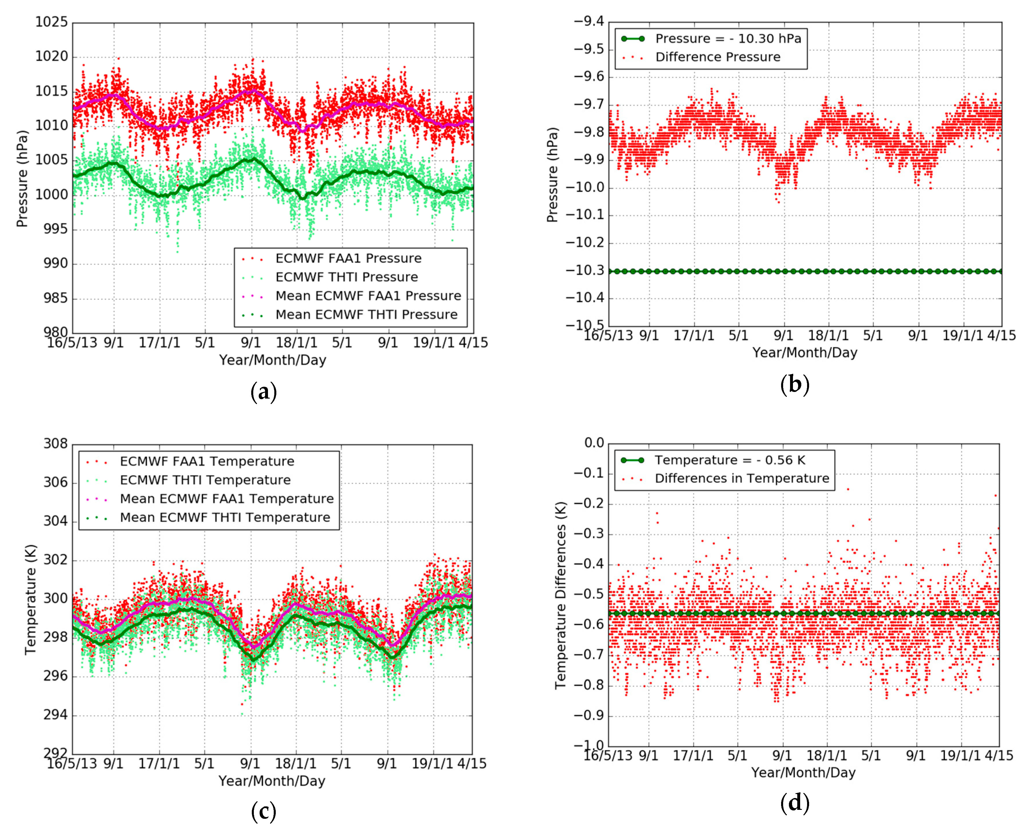
Figure 5.
Comparisons of THTI (light-green dots) and FAA1 (red dots) ECMWF pressures, and monthly averaged estimates of the THTI (green dots) and FAA1 (magenta dots) ECMWF pressures (a) and temperatures (c), and the pressure difference from standard model (−10.30 hPa, green dots) and the corresponding pressure difference from ECMWF (b) the temperature difference from standard model (−0.56 K, green dots) and the corresponding temperature difference from ECMWF (d). The temporal resolution is six hours.
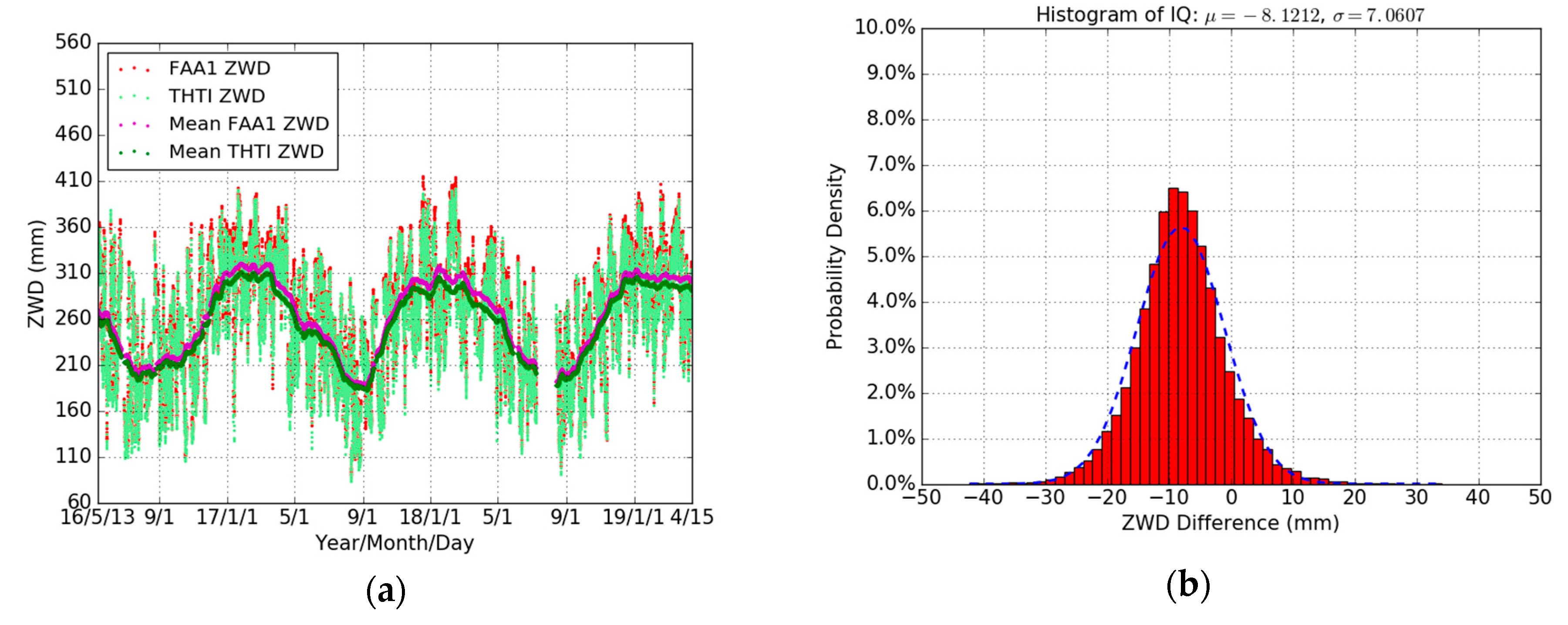
Figure 6.
Comparisons of THTI ZWD (light-green dots) with FAA1 ZWD (red dots), and monthly averaged estimates of the THTI ZWD (green dots) and FAA1 ZWD (magenta dots) (a) and the ZWD difference between them (b). The temporal resolution is one hour.
Figure 6.
Comparisons of THTI ZWD (light-green dots) with FAA1 ZWD (red dots), and monthly averaged estimates of the THTI ZWD (green dots) and FAA1 ZWD (magenta dots) (a) and the ZWD difference between them (b). The temporal resolution is one hour.
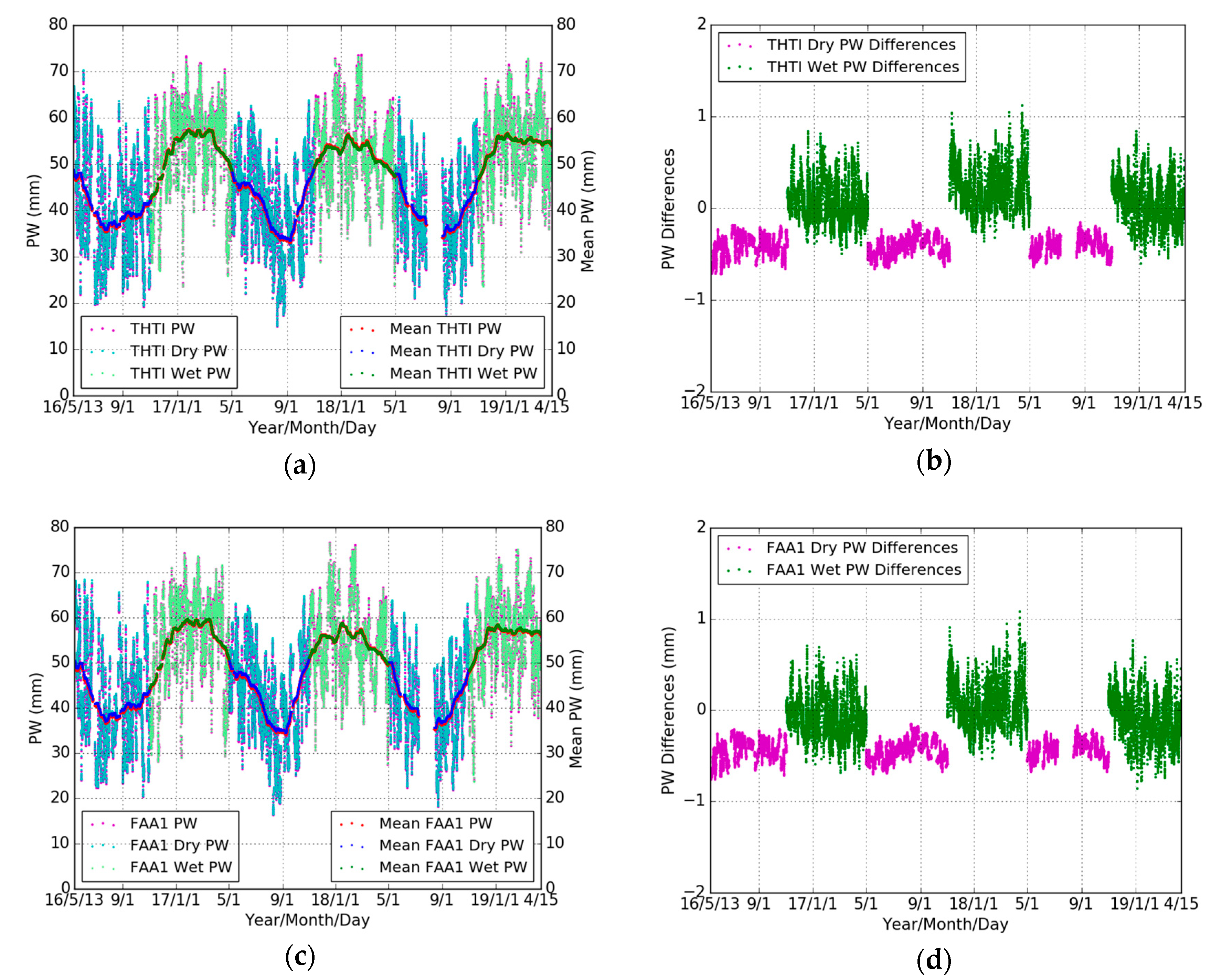
Figure 7.
Comparisons of THTI PW values (magenta dots) based on all seasons’ model with THTI Dry PW (cyan dots) and THTI Wet PW (light-green dots) based on the corresponding dry and wet season’s models, and monthly averaged estimates of the THTI PW (red dots) and THTI Dry PW (blue dots) and THTI Wet PW (green dots) (a) and their differences (b), and comparisons of FAA1 PW (magenta dots) based on all seasons’ model with FAA1 Dry PW (cyan dots) and FAA1 Wet PW (light-green dots) based on the corresponding dry and wet season’s models, and monthly averaged estimates of the FAA1 PW (red dots) and FAA1 Dry PW (blue dots) and FAA1 Wet PW (green dots) (c) and their differences (d).
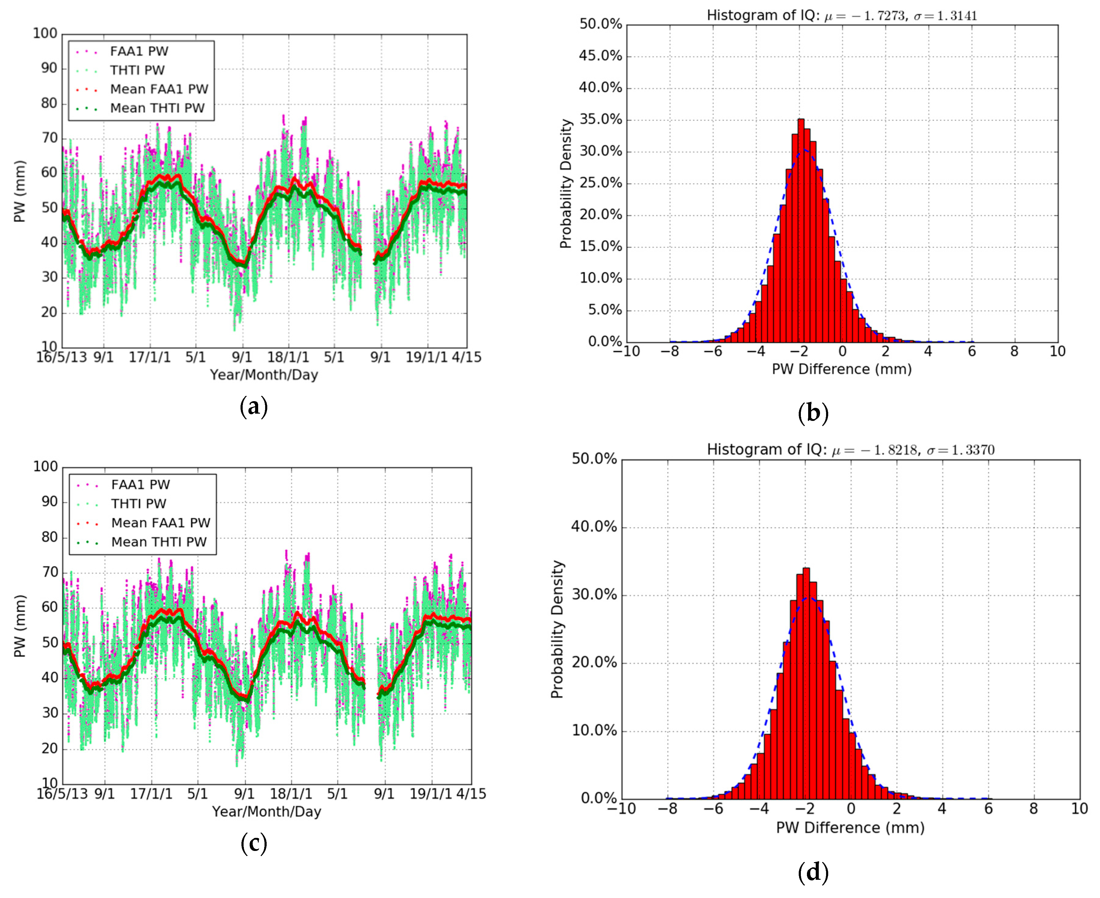
Figure 8.
Comparisons of THTI PW (light-green dots) with FAA1 PW estimates (magenta dots) based on an all seasons’ model, and monthly averaged estimates of the THTI PW (green dots) and FAA1 PW (red dots) (a) and their differences (b), and based on seasonal models (c) and their differences (d).
Figure 8.
Comparisons of THTI PW (light-green dots) with FAA1 PW estimates (magenta dots) based on an all seasons’ model, and monthly averaged estimates of the THTI PW (green dots) and FAA1 PW (red dots) (a) and their differences (b), and based on seasonal models (c) and their differences (d).
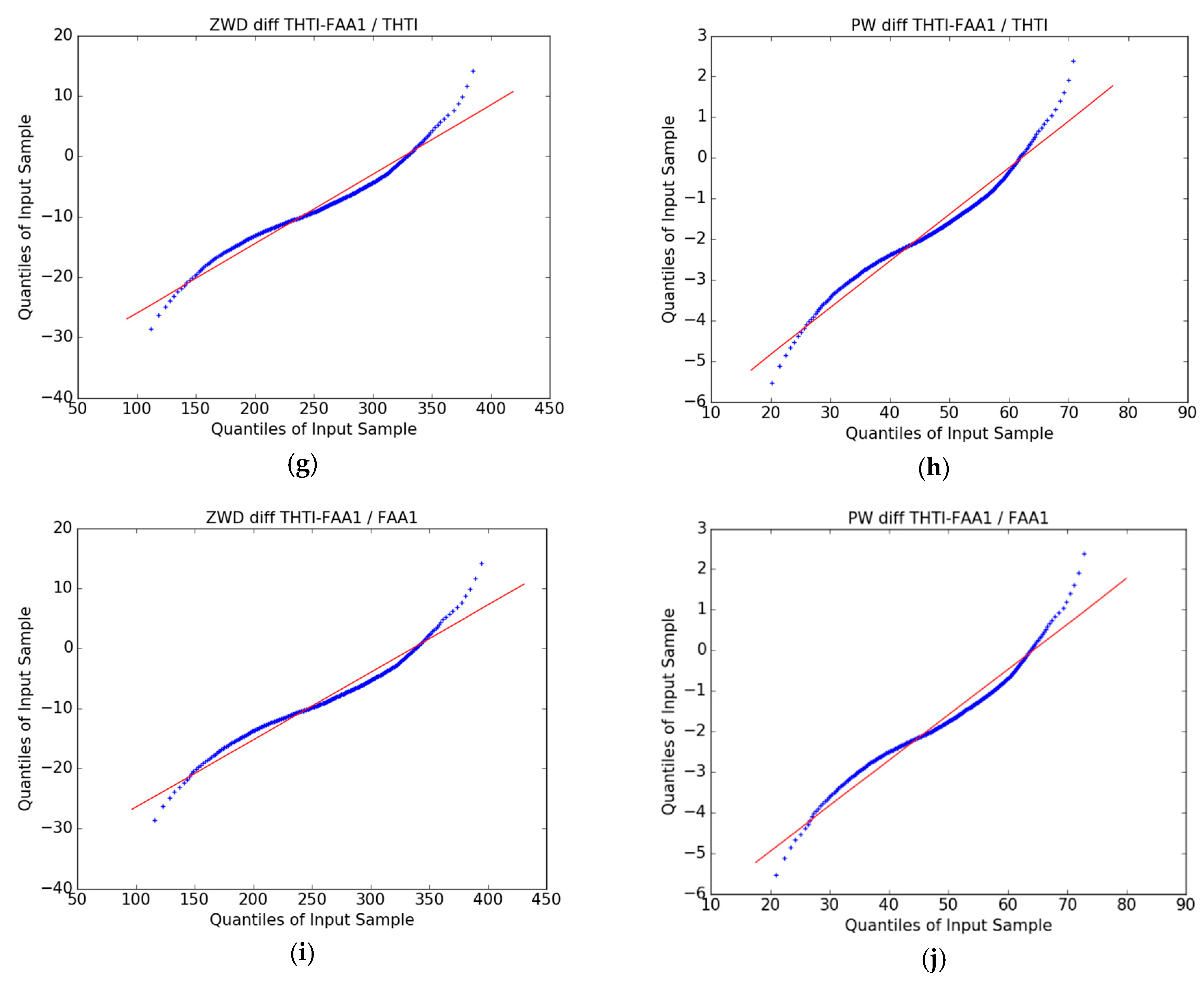
Figure 9.
QQ plots of THTI ZWD (a) and THTI PW (b) with normal law, FAA1 ZWD (c) and FAA1 PW (d) with normal law, and QQ plots of cross-comparisons between THTI and FAA1, their ZWD difference with normal law (e) and their PW difference with normal law (f), and their ZWD difference with THTI ZWD (g) and their PW difference with THTI PW (h), and their ZWD differences with FAA1 ZWD (i), and their PW differences with FAA1 PW (j). The red lines are linear quartile–quartile estimates of the fit to be expected if the two distributions are linearly related.
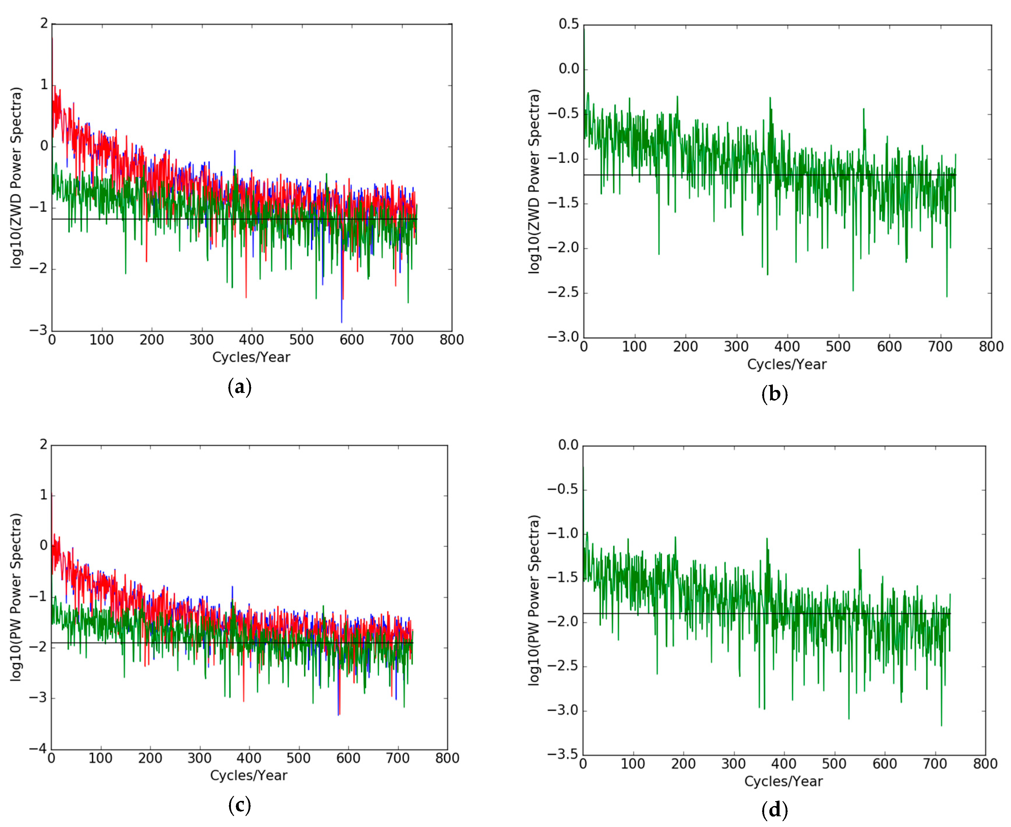
Figure 10.
The power spectra of THTI ZWD (blue curve), FAA1 ZWD (red curve) and their differences (green curve) (a), and (b) the power spectrum of ZWD differences (enlarged green curve of (a)), the black line is the spectrum of a white noise matching the data noise; and the power spectra of THTI PW (blue curve), FAA1 PW (red curve) and their differences (green curve) (c), and (d) the power spectra of PW differences (enlarged green curve of (c)). The black line is the spectrum of white noise. Sub-diurnal variations cannot be retrieved, as they are buried in the noise.
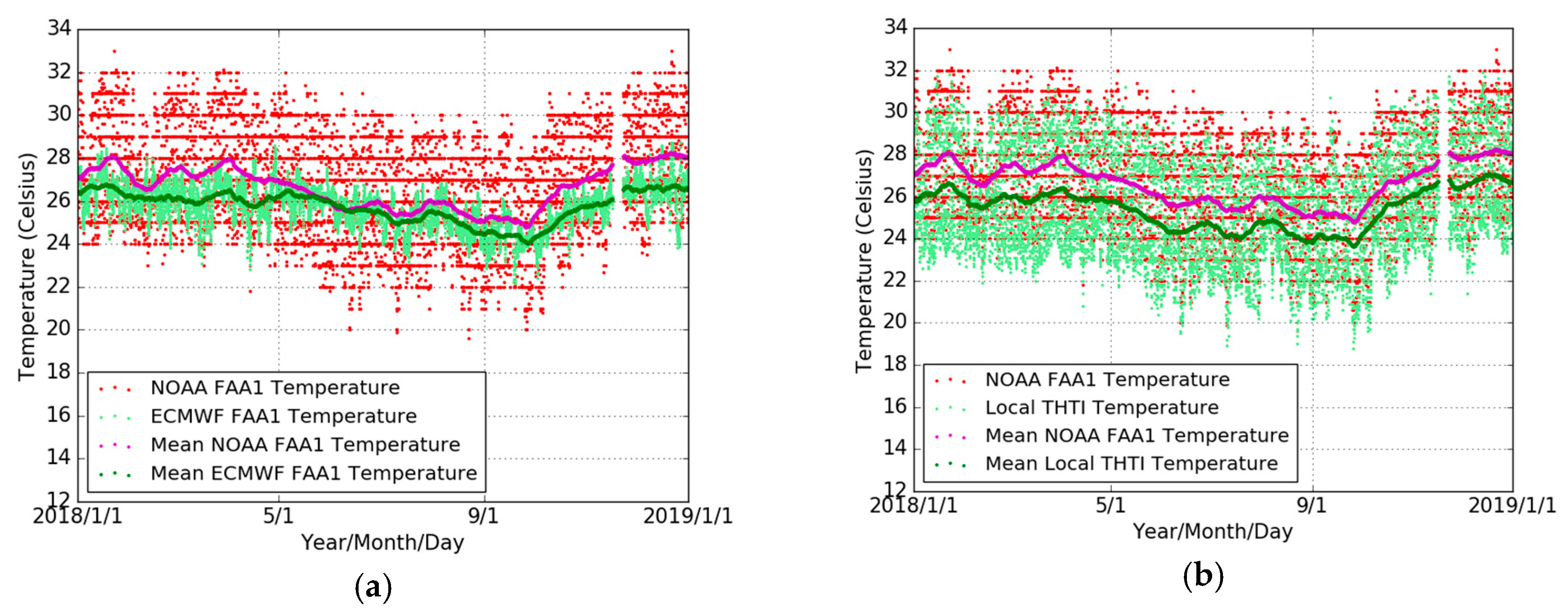
Figure 11.
Comparisons of surface temperature from NOAA (red dots) and ECMWF (light-green dots), and 10 days averaged temperature estimates from NOAA (magenta dots) and ECMWF (green dots) (a), and the comparison of local THTI (light-green dots) temperature and NOAA FAA1 (red dots) temperature, and 10 days averaged temperature estimates of local THTI (green dots) and NOAA FAA1 (magenta dots) (b). The comparison is done for the whole year of 2018.
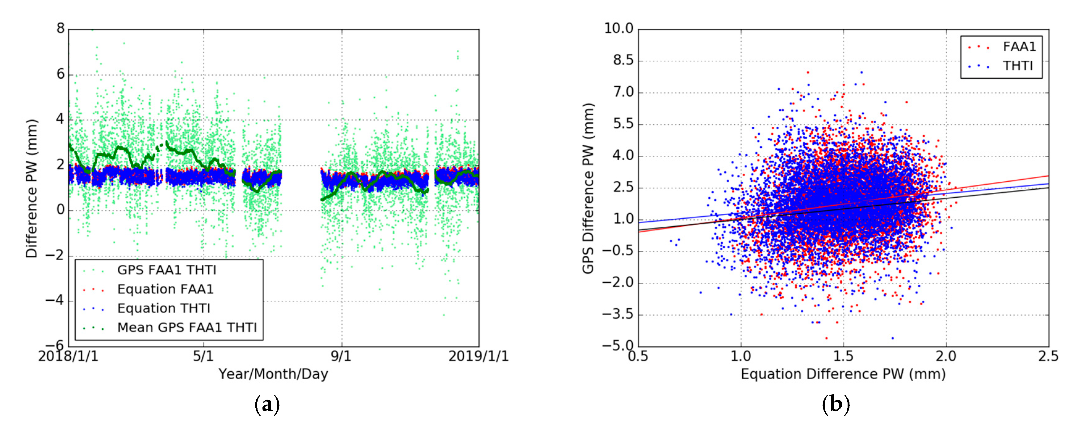
Figure 12.
Comparisons of PW differences from GPS (FAA1-THTI, light-green dots) and their monthly averaged values (green dots) and exponentially derived PW (PWE) estimates (Equation (15)), with ns values for THTI (blue dots) and FAA1 (red dots) (a), and the respective fits of GPS-PW differences based on Equation (15) (b). The black line corresponds to the one-to-one relationship between the GPS-PW differences and the PWE differences.
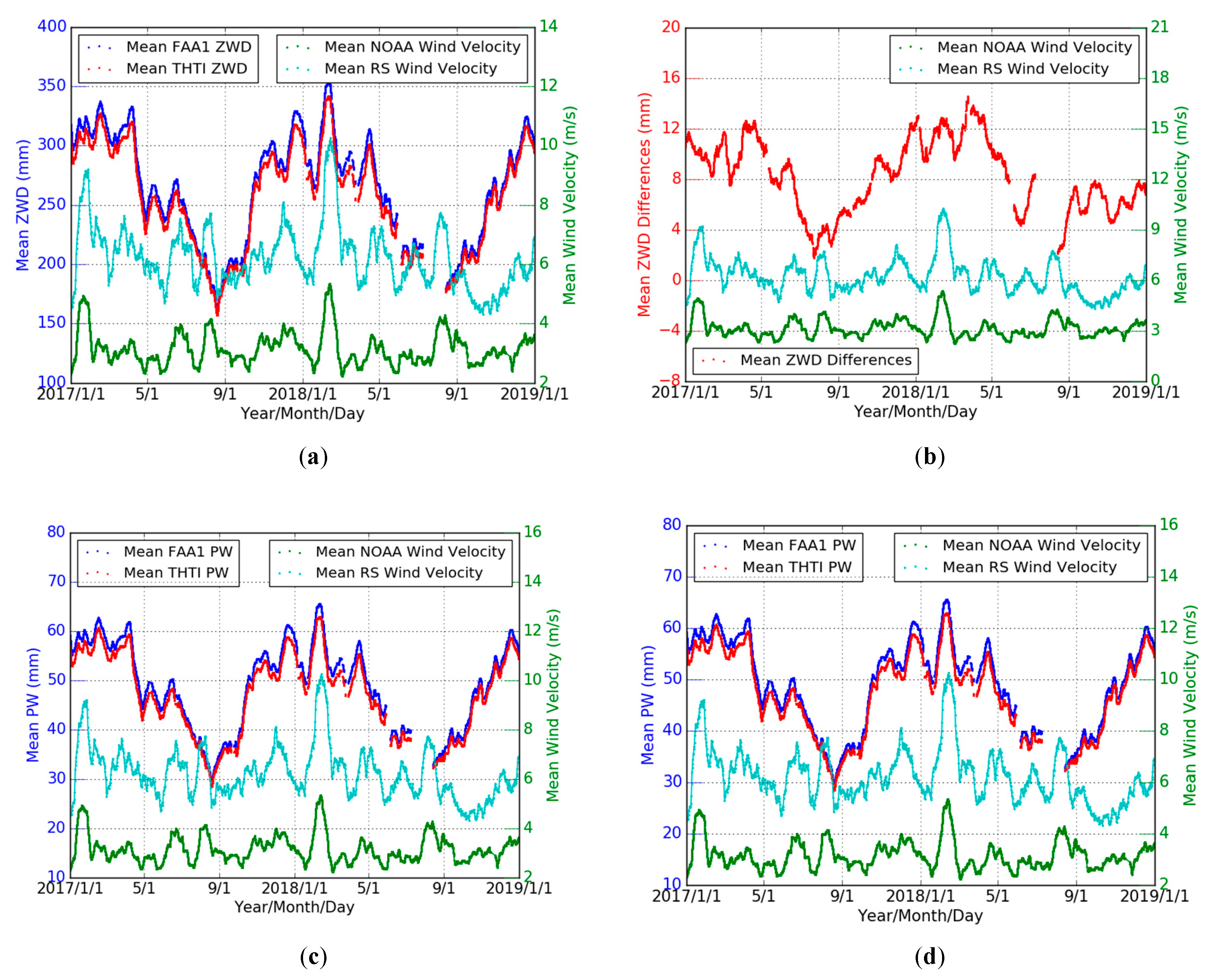
Figure 13.
Variations of the averaged ZWD values of THTI (red dots) and FAA1 (blue dots) and the wind velocity values from NOAA (green dots) and RS (cyan dots) (a), and for PW values (c), and the variations of the corresponding averaged ZWD differences (red dots) between two stations with the wind velocity from NOAA (green dots) and RS (cyan dots) (b), and for PW differences (d).
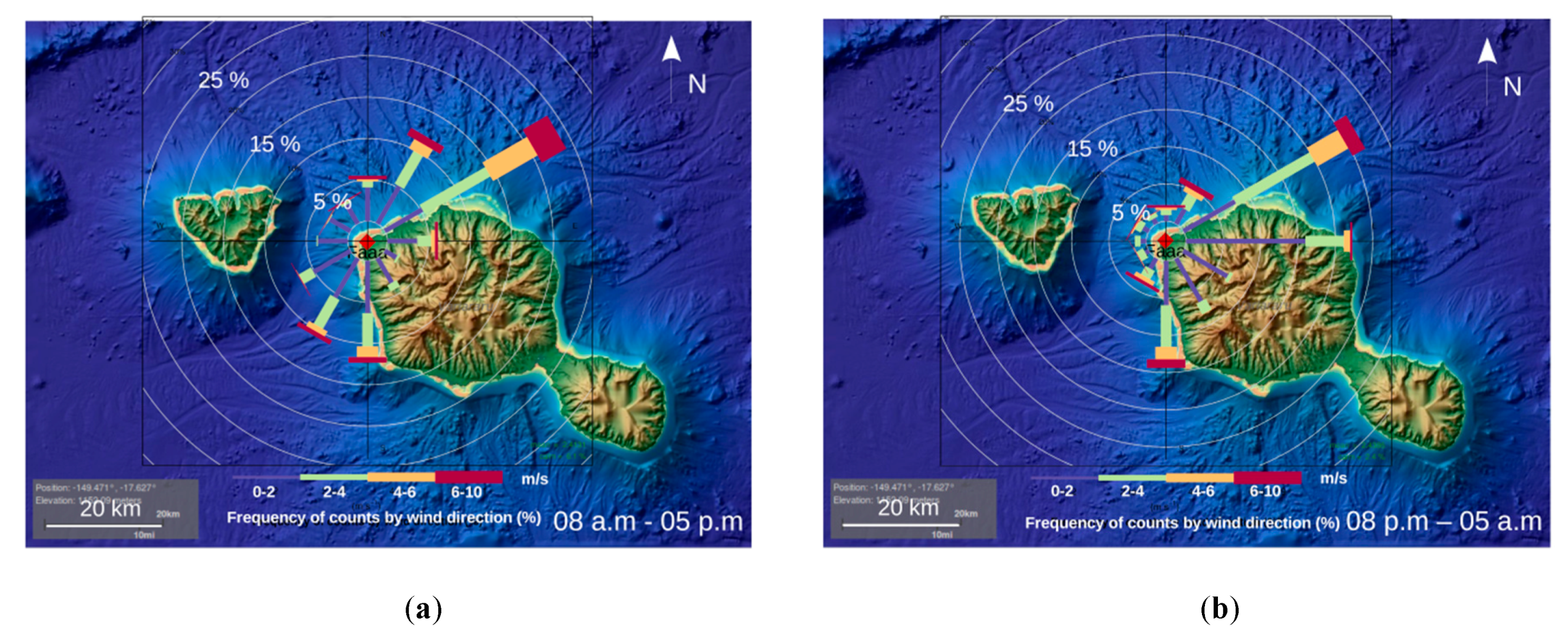
Figure 14.
Ten m wind rose for 2017 and 2018 at FAA1 station: (a) during the day time from 8:00 to 17:00, and (b) during the night time from 20:00 to 05:00.
Figure 14.
Ten m wind rose for 2017 and 2018 at FAA1 station: (a) during the day time from 8:00 to 17:00, and (b) during the night time from 20:00 to 05:00.
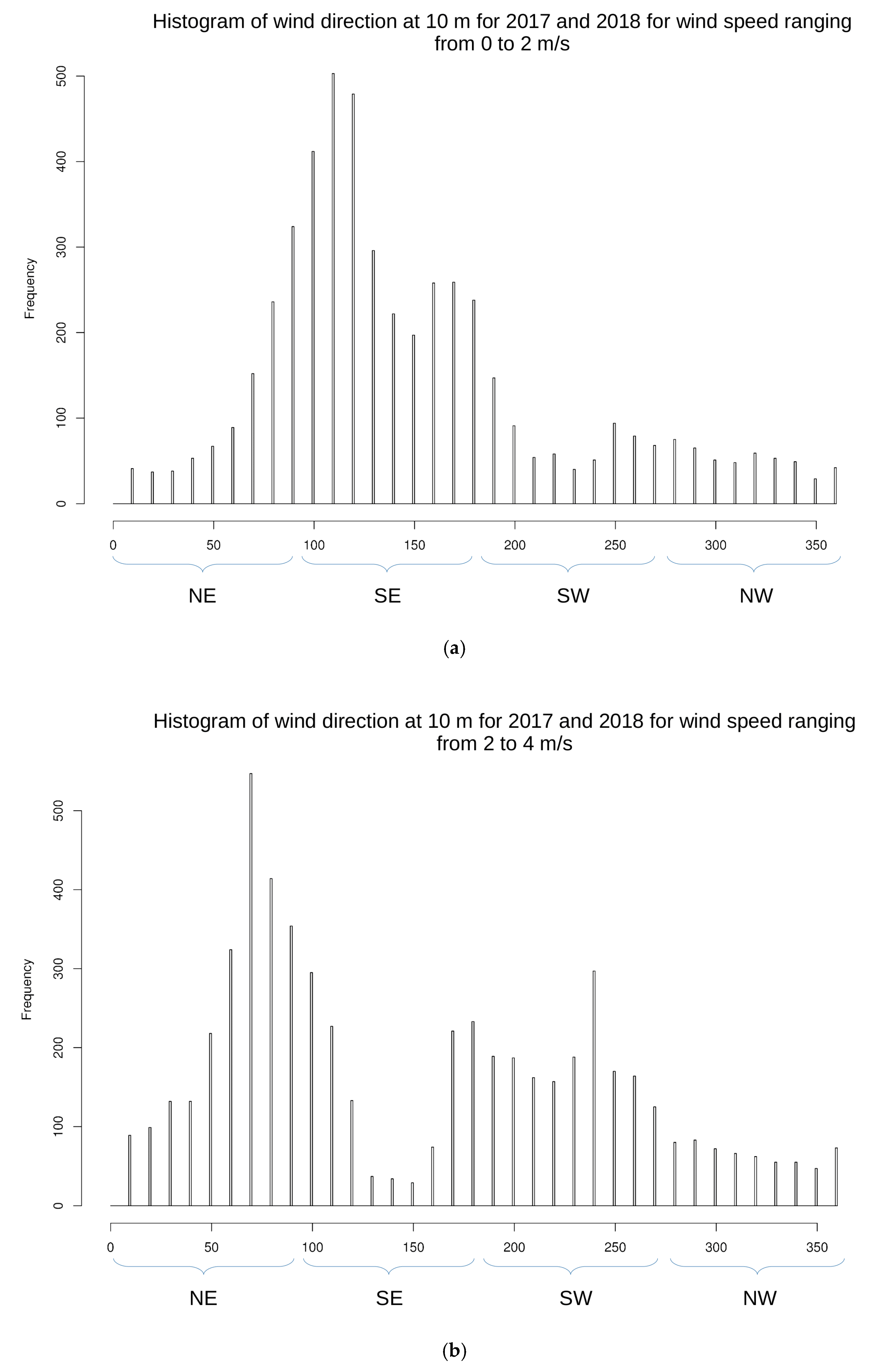
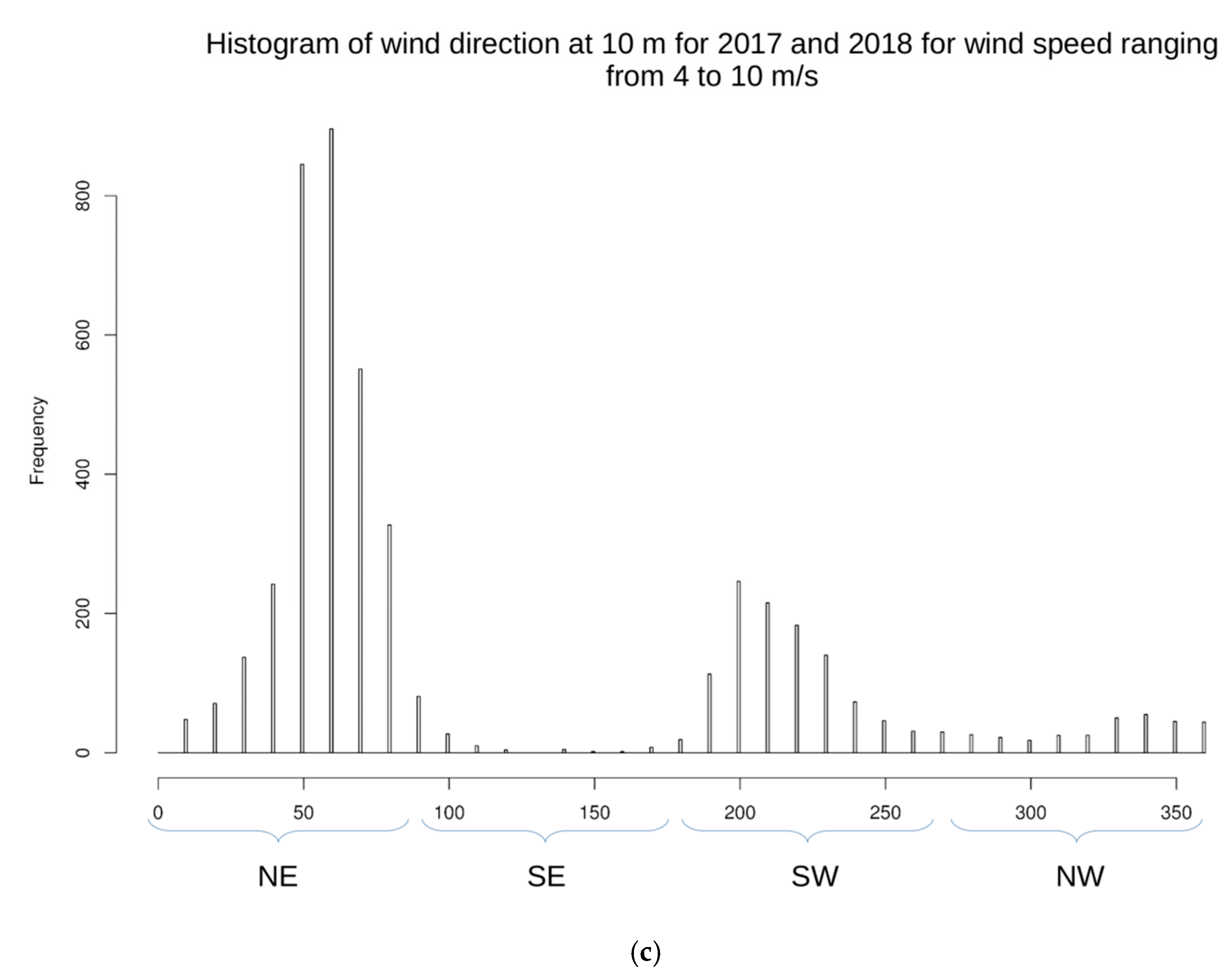
Figure 15.
Histogram of 10 m wind direction at FAA1 for 2017–2018 (
a) for 0 to 2 m/s, and (
b) for 2 to 4 m/s, and (
c) for 4 to 10 m/s. North-east direction is indicated by “NE” and spans 0° to 90°, south-east direction is indicated by “SE” and spans 90° to 180°, south-west direction is indicated by “SW” and spans 180° to 270°, north-west direction is indicated by “NW” and spans 270° to 360°. The corresponding wind rose is shown in
Figure 14.
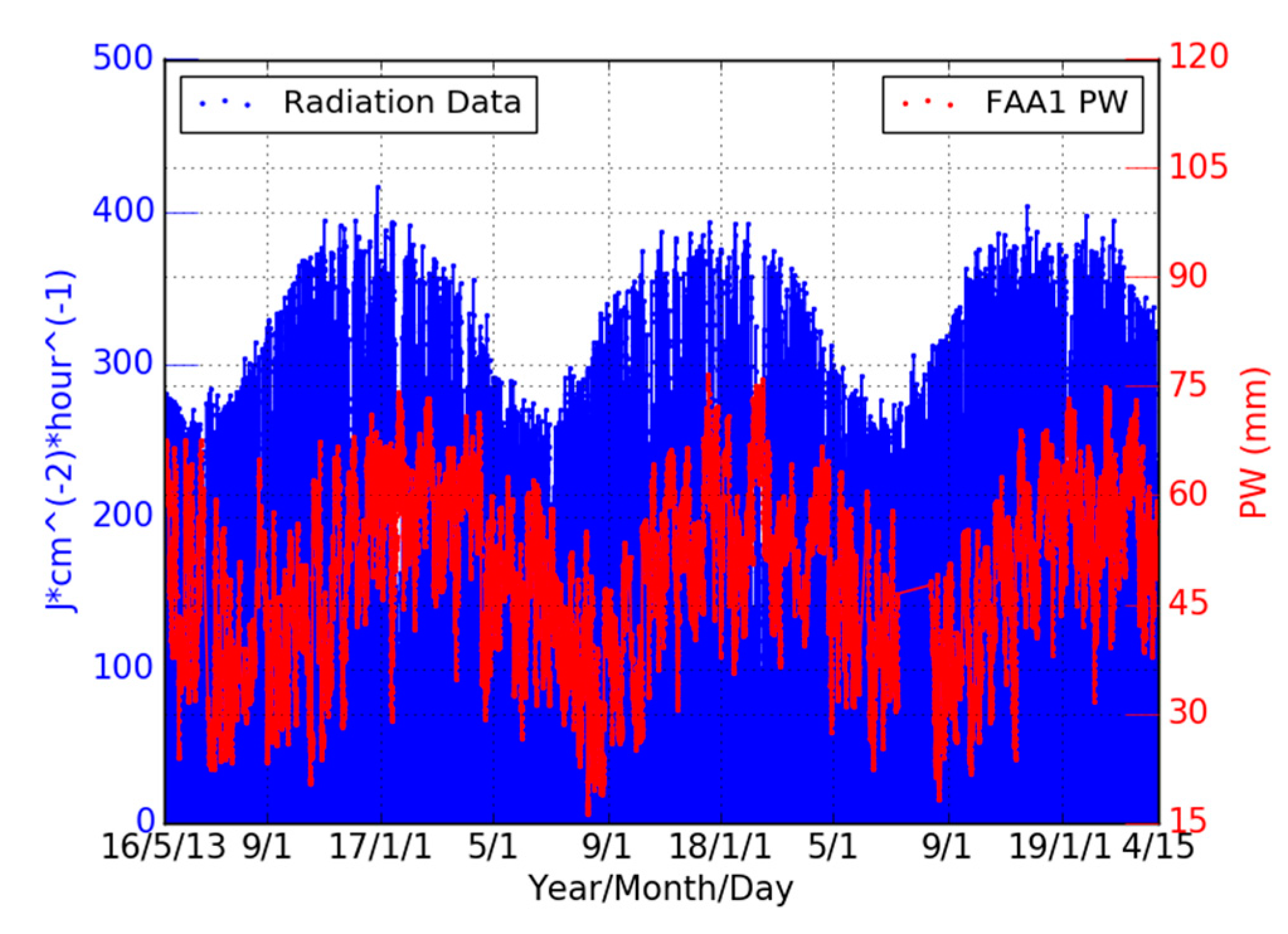
Figure 16.
Hourly insolation variation from the pyranometer collocated with the FAA1 station, showing the strong annual signature driven by the Sun sky trajectory. The PW data relative to FAA1 station (see
Section 6.7) are shown in red dots. A time shift of about two months between the two series is clearly visible, probably linked to the thermal inertia of the soil or/and a time delay in the vegetation response (evapotranspiration) to the insolation.
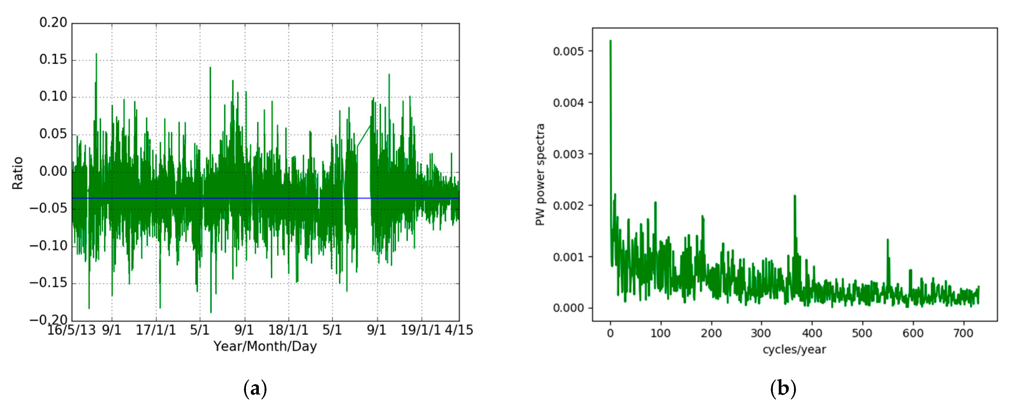
Figure 17.
(
a) Time series, over the three years of this study, of the ratio of PW values, defined as (PW(THTI)−PW(FAA1))/PW(FAA1). The mean value of this ratio is −0.0355 ± 0.0002. (
b) Fourier analysis of the time series of subfigure (
a). The annual component is largely attenuated with respect to the annual component in the time series of (PW(THTI)−PW(FAA1)), as seen in
Figure 10d, pointing to a common factor with annual periodicity in the original time series of PW values for the two sites.
Table 1.
Characteristics of our Global Positioning System (GPS) data processing and International Global Navigation Satellite System Service (IGS) data analysis centers.
Table 1.
Characteristics of our Global Positioning System (GPS) data processing and International Global Navigation Satellite System Service (IGS) data analysis centers.
| | Our GPS Data Processing | IGS Products |
|---|
| Ephemerides, satellite clocks | CODE final | IGS final |
| Approach | PPP | PPP |
| Sampling interval | 300 s | 300 s |
| Elevation cut-off angle | 3 degrees | 7 degrees |
| Mapping function | Wet Vienna mapping function 1 (VMF1) | Wet global mapping function (GMF) |
| A priori zenith tropospheric delay (ZTD) model | European Center for Medium-Range Weather Forecasts (ECMWF)-based dry VMF1 | Global pressure model (GPT) |
| Ocean loading | Applied | Applied |
| Atmospheric loading | Applied | Applied |
| Observables | Zero differences | Double differences |
| ZTD estimation interval | 1 hour | 5 minutes |
| Software version | Bernese 5.2 | Bernese 5.0/Bernese 5.2 |
Table 2.
models for all-season and two different tropical seasons (dry and wet) [
20].
Table 2.
models for all-season and two different tropical seasons (dry and wet) [
20].
| Intercept | Sigma | Slope | Sigma |
|---|
| All seasons | −476.4 | 145.6 | 2.68 | 0.49 |
| Dry season | −535.7 | 252.9 | 2.89 | 0.85 |
| Wet season | −979.7 | 226.9 | 4.36 | 0.76 |
Table 3.
Statistical summary for the comparison between GPS THTI/FAA1 ZTD and IGS THTI/FAA1 ZTD (IGS minus GPS) in terms of maximum (max), minimum (min), bias, root mean square (RMS) and standard deviation (STD), relative to
Figure 2b,d.
Table 3.
Statistical summary for the comparison between GPS THTI/FAA1 ZTD and IGS THTI/FAA1 ZTD (IGS minus GPS) in terms of maximum (max), minimum (min), bias, root mean square (RMS) and standard deviation (STD), relative to
Figure 2b,d.
| Difference | Max (mm) | Min (mm) | Bias (mm) | RMS (mm) | STD (mm) | Data Points |
|---|
| THTI | 17.09 | 17.06 | 0.45 | 5.37 | 5.35 | 24279 |
| FAA1 | 26.76 | 26.75 | 0.87 | 8.21 | 8.16 | 23741 |
Table 4.
Statistical summary for the comparison between GPS/IGS THT ZTD and GPS/IGS FAA1 ZTD (FAA1 minus THTI) in terms of max, min, bias, RMS, and STD, relative to
Figure 3b,d.
Table 4.
Statistical summary for the comparison between GPS/IGS THT ZTD and GPS/IGS FAA1 ZTD (FAA1 minus THTI) in terms of max, min, bias, RMS, and STD, relative to
Figure 3b,d.
| Difference | Max (mm) | Min (mm) | Bias (mm) | RMS (mm) | STD (mm) | Data Points |
|---|
| Our FAA1-THTI | 64.53 | 11.84 | 30.45 | 31.25 | 7.03 | 22679 |
| IGS FAA1-THTI | 71.90 | 1.20 | 31.71 | 32.17 | 5.42 | 22679 |
Table 5.
Statistical summary for the comparison between ECMWF pressure/temperature and local pressure/temperature, and ZHD derived from two kinds of pressure data (ECMWF minus local) in terms of max, min, bias, RMS, and STD during the whole year of 2018.
Table 5.
Statistical summary for the comparison between ECMWF pressure/temperature and local pressure/temperature, and ZHD derived from two kinds of pressure data (ECMWF minus local) in terms of max, min, bias, RMS, and STD during the whole year of 2018.
| Difference | Max | Min | Bias | RMS | STD | Data Points |
|---|
| Pressure (hPa) | 2.68 | 2.23 | 0.58 | 0.87 | 0.65 | 8726 |
| Temperature (K) | 6.33 | 5.43 | 0.26 | 2.21 | 2.19 | 8726 |
| DZHD (mm) | 5.08 | 6.12 | 1.32 | 1.99 | 1.49 | 8726 |
Table 6.
Statistical summary for the comparison between THTI and FAA1 ECMWF pressure/temperature (THTI minus FAA1) in terms of max, min, bias, RMS, and STD, relative to
Figure 5b,d.
Table 6.
Statistical summary for the comparison between THTI and FAA1 ECMWF pressure/temperature (THTI minus FAA1) in terms of max, min, bias, RMS, and STD, relative to
Figure 5b,d.
| Difference | Max | Min | Bias | RMS | STD | Data Points |
|---|
| Pressure (hPa) | 9.64 | 10.05 | 9.81 | 9.81 | 0.06 | 4264 |
| Temperature (K) | 0.15 | 0.85 | 0.60 | 0.60 | 0.09 | 4264 |
Table 7.
Statistical summary for the comparison between our THTI ZWDs and our FAA1 ZWDs (THTI minus FAA1) in terms of max, min, bias, RMS, and STD, relative to
Figure 6b.
Table 7.
Statistical summary for the comparison between our THTI ZWDs and our FAA1 ZWDs (THTI minus FAA1) in terms of max, min, bias, RMS, and STD, relative to
Figure 6b.
| Difference | Max (mm) | Min (mm) | Bias (mm) | RMS (mm) | STD (mm) | Data Points |
|---|
| ZWD | 34.10 | 42.22 | 8.12 | 10.76 | 7.06 | 22649 |
Table 8.
Statistical summary for the comparisons between THTI/FAA1 PW based on all seasons’
model and THTI/FAA1 PW based on seasonal
model (all seasons’ minus seasonal) in terms of max, min, bias, RMS, and STD, relative to
Figure 7b,d.
Table 8.
Statistical summary for the comparisons between THTI/FAA1 PW based on all seasons’
model and THTI/FAA1 PW based on seasonal
model (all seasons’ minus seasonal) in terms of max, min, bias, RMS, and STD, relative to
Figure 7b,d.
| Difference | Max (mm) | Min (mm) | Bias (mm) | RMS (mm) | STD (mm) | Data Points |
|---|
| THTI Dry | −0.13 | −0.72 | −0.41 | 0.42 | 0.11 | 10,875 |
| THTI Wet | 1.13 | −0.60 | 0.13 | 0.27 | 0.24 | 11,774 |
| FAA1 Dry | −0.15 | −0.76 | −0.43 | 0.45 | 0.11 | 10,875 |
| FAA1 Wet | 1.09 | −0.86 | −0.03 | 0.25 | 0.25 | 11,774 |
Table 9.
Statistical summary for the comparison between THTI and FAA1 PW estimates based on an all seasons’
model and based on seasonal
models (THTI minus FAA1) in terms of max, min, bias, RMS, and STD, relative to
Figure 8b,d.
Table 9.
Statistical summary for the comparison between THTI and FAA1 PW estimates based on an all seasons’
model and based on seasonal
models (THTI minus FAA1) in terms of max, min, bias, RMS, and STD, relative to
Figure 8b,d.
| Difference | Max (mm) | Min (mm) | Bias (mm) | RMS (mm) | STD (mm) | Data Points |
|---|
| All Seasons | 6.11 | −7.97 | −1.73 | 2.17 | 1.31 | 22649 |
| Seasonal | 6.16 | −8.05 | −1.82 | 2.26 | 1.34 | 22649 |
Table 10.
Statistical summary for the comparison between NOAA and ECMWF at FAA1 station (NOAA minus ECMWF) and the comparison of local THTI temperature with NOAA FAA1 temperature (NOAA FAA1 minus local THTI) in terms of max, min, bias, RMS, and STD, for the whole year of 2018.
Table 10.
Statistical summary for the comparison between NOAA and ECMWF at FAA1 station (NOAA minus ECMWF) and the comparison of local THTI temperature with NOAA FAA1 temperature (NOAA FAA1 minus local THTI) in terms of max, min, bias, RMS, and STD, for the whole year of 2018.
| Difference | Max | Min | Bias | RMS | STD | Data Points |
|---|
| FAA1 (°C) | 6.87 | −5.42 | 0.87 | 2.34 | 2.17 | 8271 |
| FAA1–THTI (°C) | 6.60 | −2.00 | 1.23 | 1.44 | 0.76 | 8271 |
Table 11.
Statistical summary for the differences of GPS-PW, PWE (FAA1) and PWE (THTI) in terms of max, min, bias, RMS, and STD, relative to
Figure 12a.
Table 11.
Statistical summary for the differences of GPS-PW, PWE (FAA1) and PWE (THTI) in terms of max, min, bias, RMS, and STD, relative to
Figure 12a.
| Difference | Max (mm) | Min (mm) | Bias (mm) | RMS (mm) | STD (mm) | Data Points |
|---|
| GPS-PW | 8.0 | −4.59 | 1.75 | 2.24 | 1.39 | 6799 |
| PWE (FAA1) | 2.07 | 0.90 | 1.51 | 1.53 | 0.19 | 6799 |
| PWE (THTI) | 2.03 | 0.67 | 1.47 | 1.49 | 0.21 | 6799 |
Table 12.
The fits of the difference of GPS-PWs and PWEs, relative to
Figure 12b.
Table 12.
The fits of the difference of GPS-PWs and PWEs, relative to
Figure 12b.
| | Intercept | Slope | Correlation Coefficient |
|---|
| FAA1 PWEs | −0.26 ± 0.13 | 1.33 ± 0.09 | 0.18 |
| THTI PWEs | 0.39 ± 0.11 | 0.92 ± 0.08 | 0.14 |
Table 13.
The fits of PW and ZWD differences between THTI and FAA1 with wind velocity from NOAA and RS.
Table 13.
The fits of PW and ZWD differences between THTI and FAA1 with wind velocity from NOAA and RS.
| | NOAA | RS | Correlation Coefficient |
|---|
| | Intercept | Slope | Intercept | Slope | NOAA | RS |
| PW Difference | 1.17 ± 0.06 | 0.18 ± 0.02 | 0.43 ± 0.07 | 0.21 ± 0.01 | 7.55% | 16.24% |
| Mean PW Difference | 1.24 ± 0.03 | 0.16 ± 0.01 | 0.47 ± 0.03 | 0.21 ± 0.00 | 16.25% | 39.20% |
| ZWD Difference | 5.58 ± 0.34 | 0.85 ± 0.11 | 1.67 ± 0.36 | 1.05 ± 0.06 | 6.43% | 15.03% |
| Mean ZWD Difference | 5.93 ± 0.13 | 0.73 ± 0.04 | 1.85 ± 0.13 | 1.02 ± 0.02 | 14.43% | 37.94% |


