Geometrical Matching of SAR and Optical Images Utilizing ASIFT Features for SAR-based Navigation Aided Systems

 ,
,  , , ,
, , ,  and
and
Abstract
1. Introduction
2. Methodology
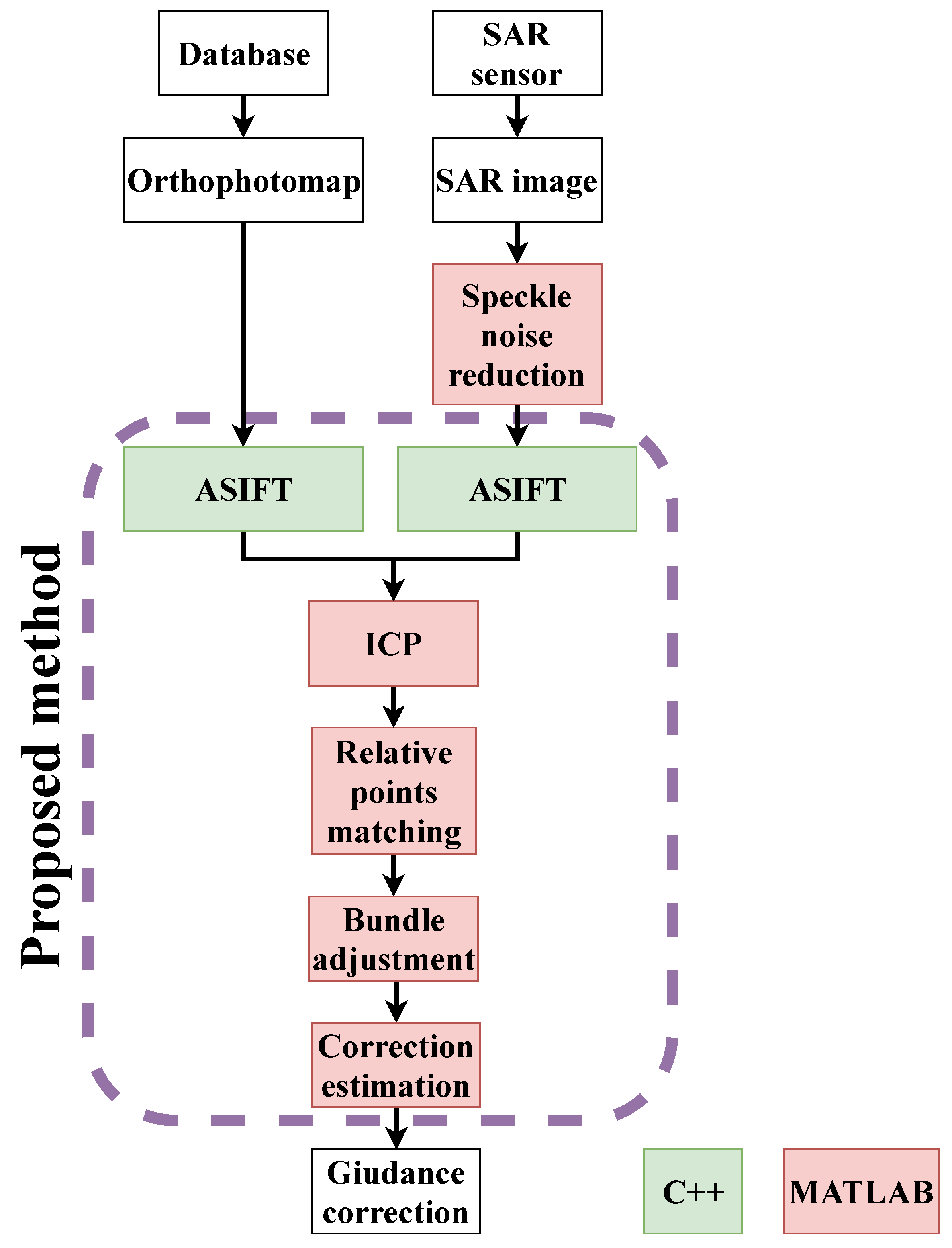
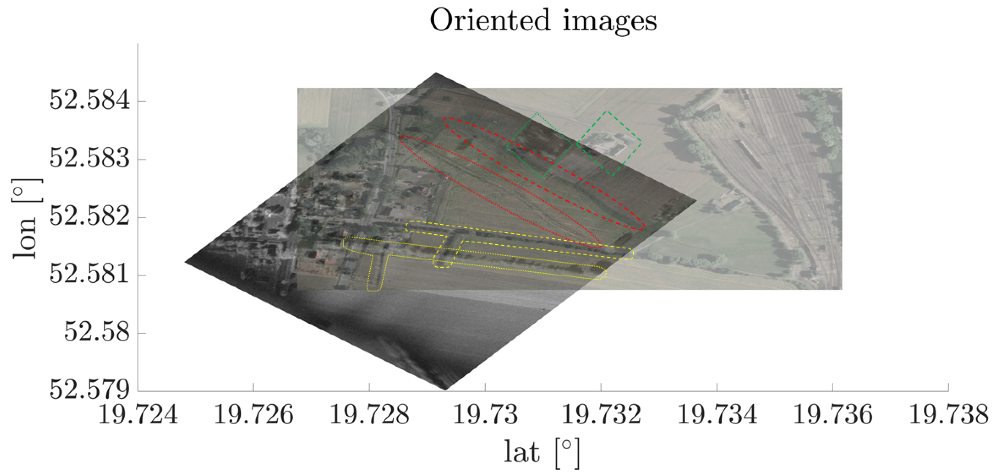
2.1. Overview of the Approach
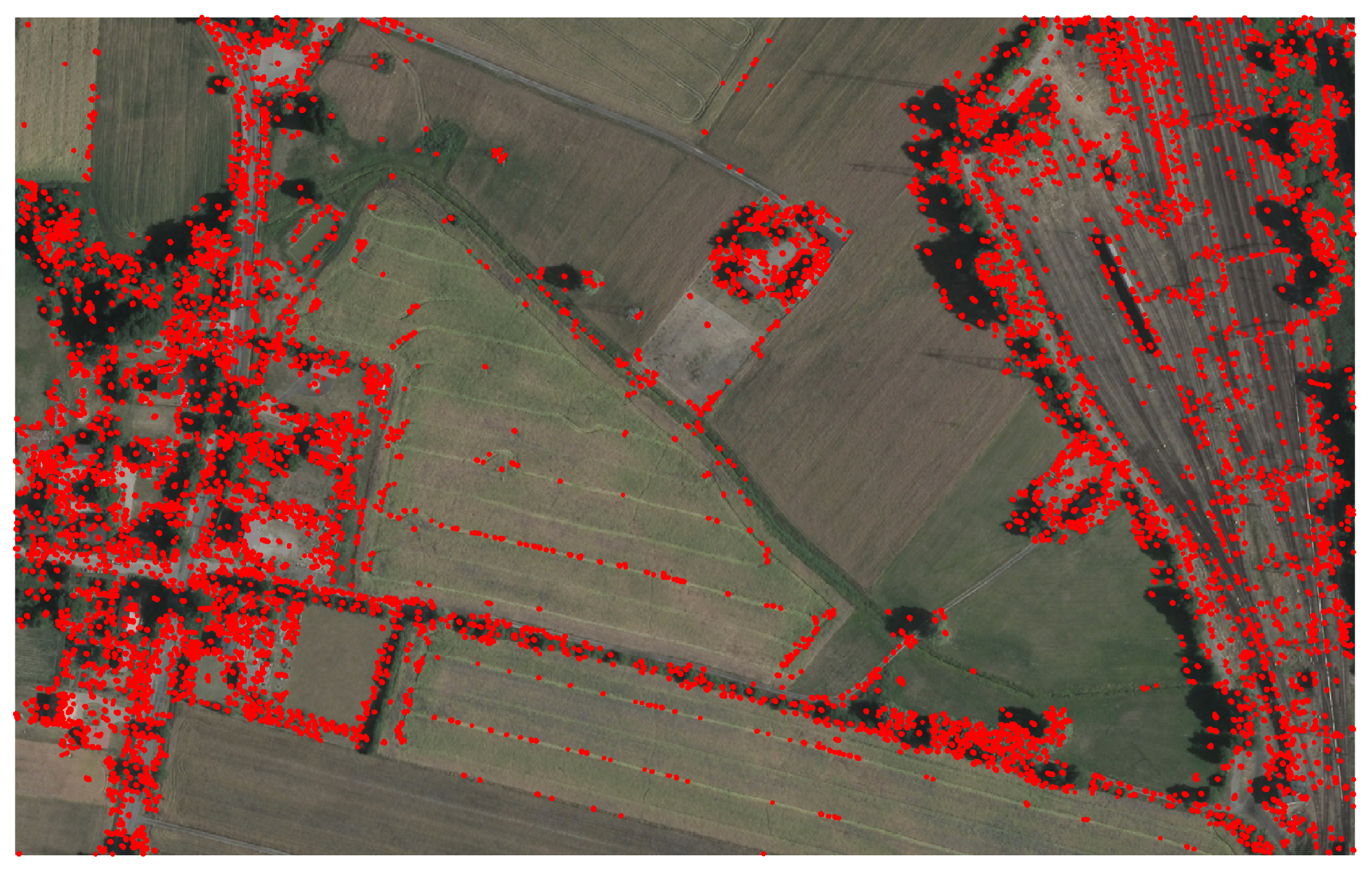
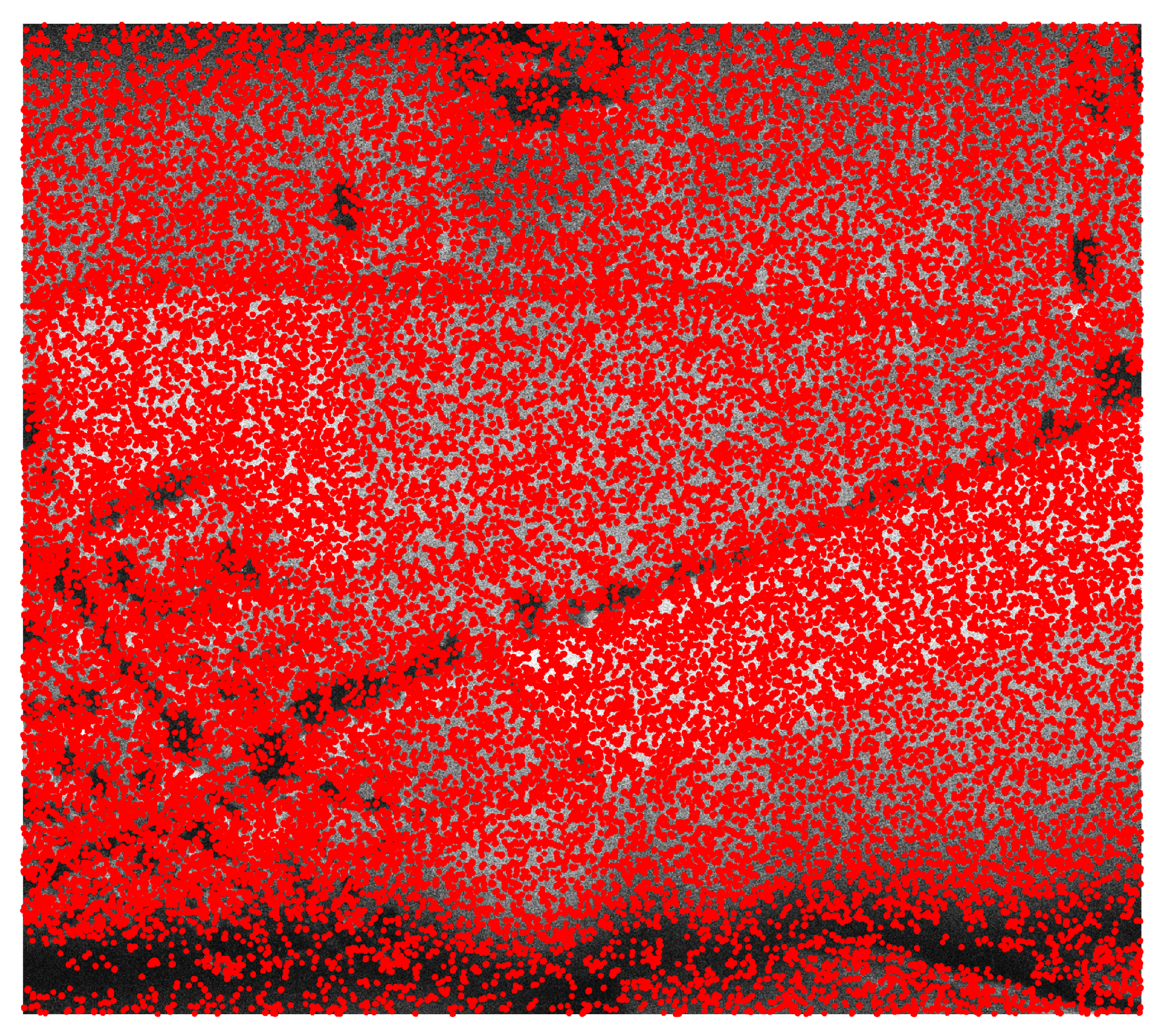
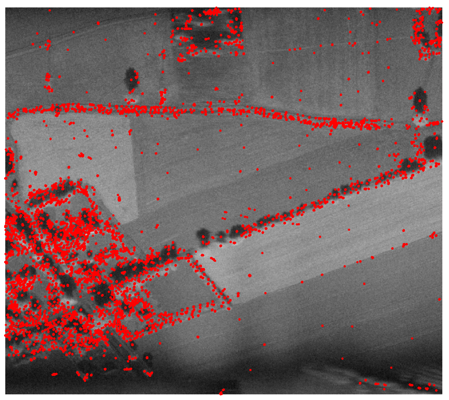
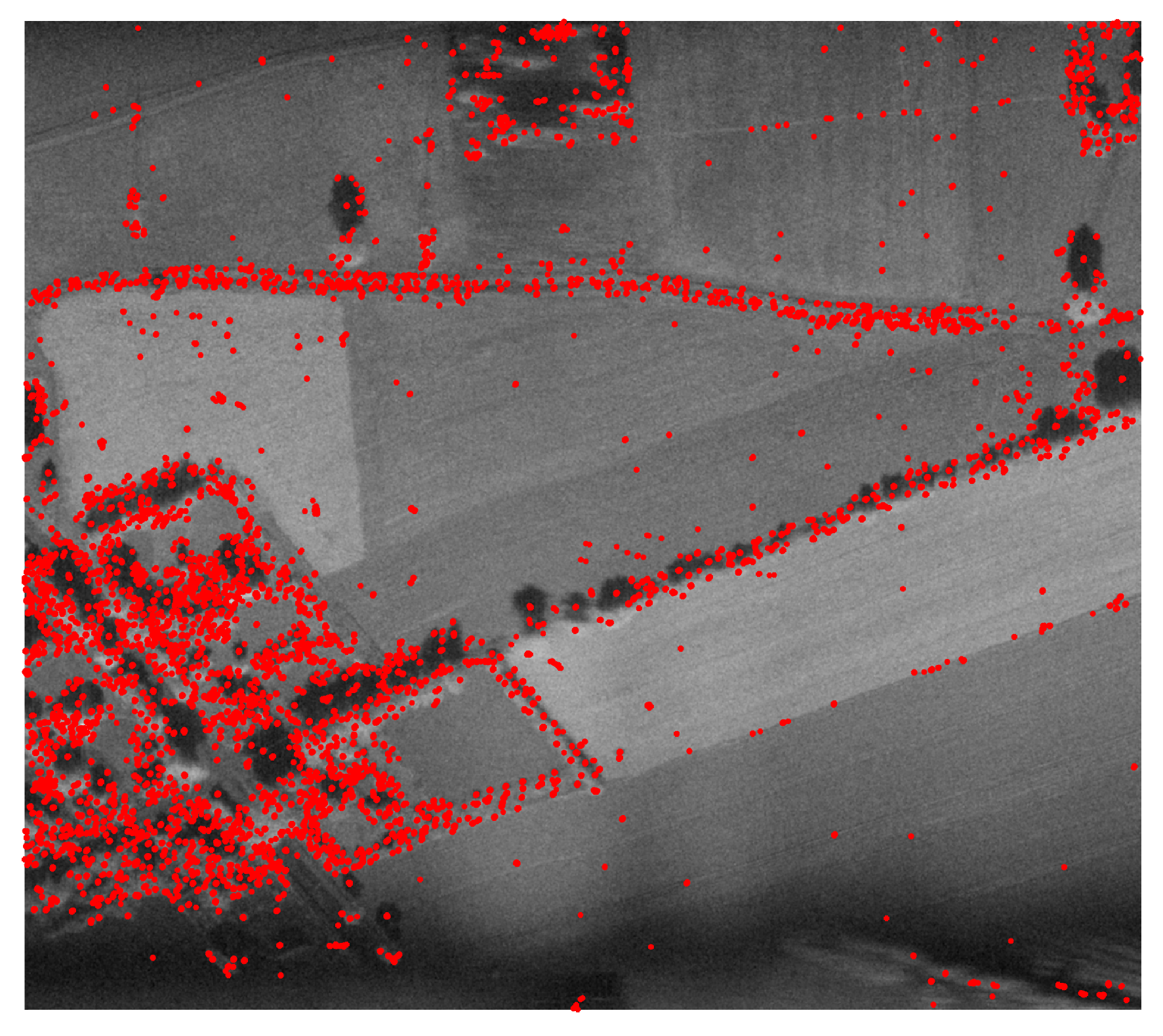
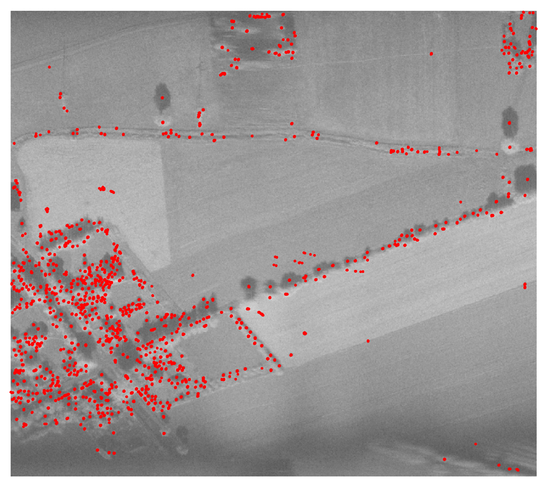
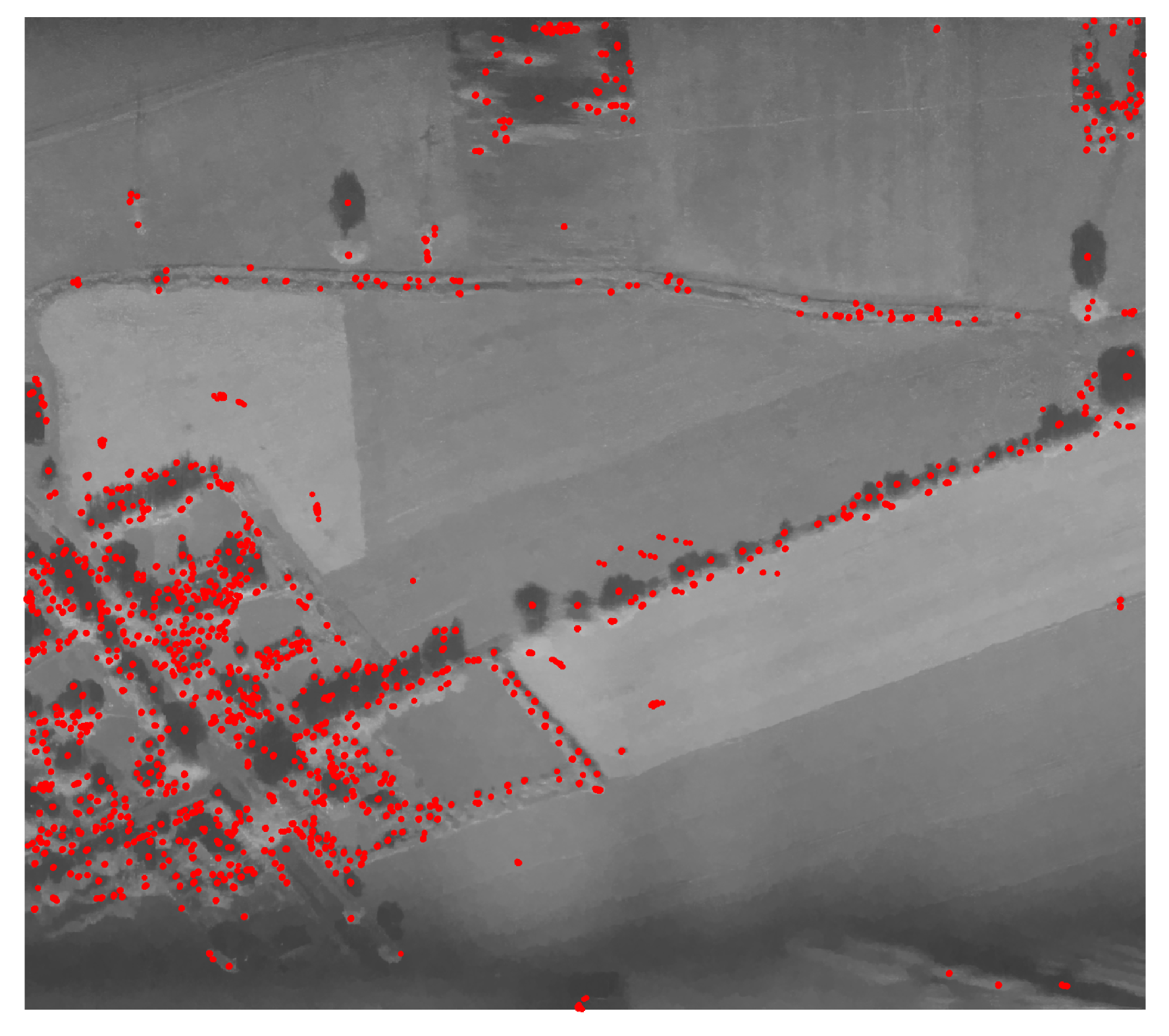
- The keypoints distributions on SAR images and orthophotomaps.
- The influence of the SAR image correction on the quality and number of the keypoints.
- The number of detected keypoints used in the final cooregistration process.
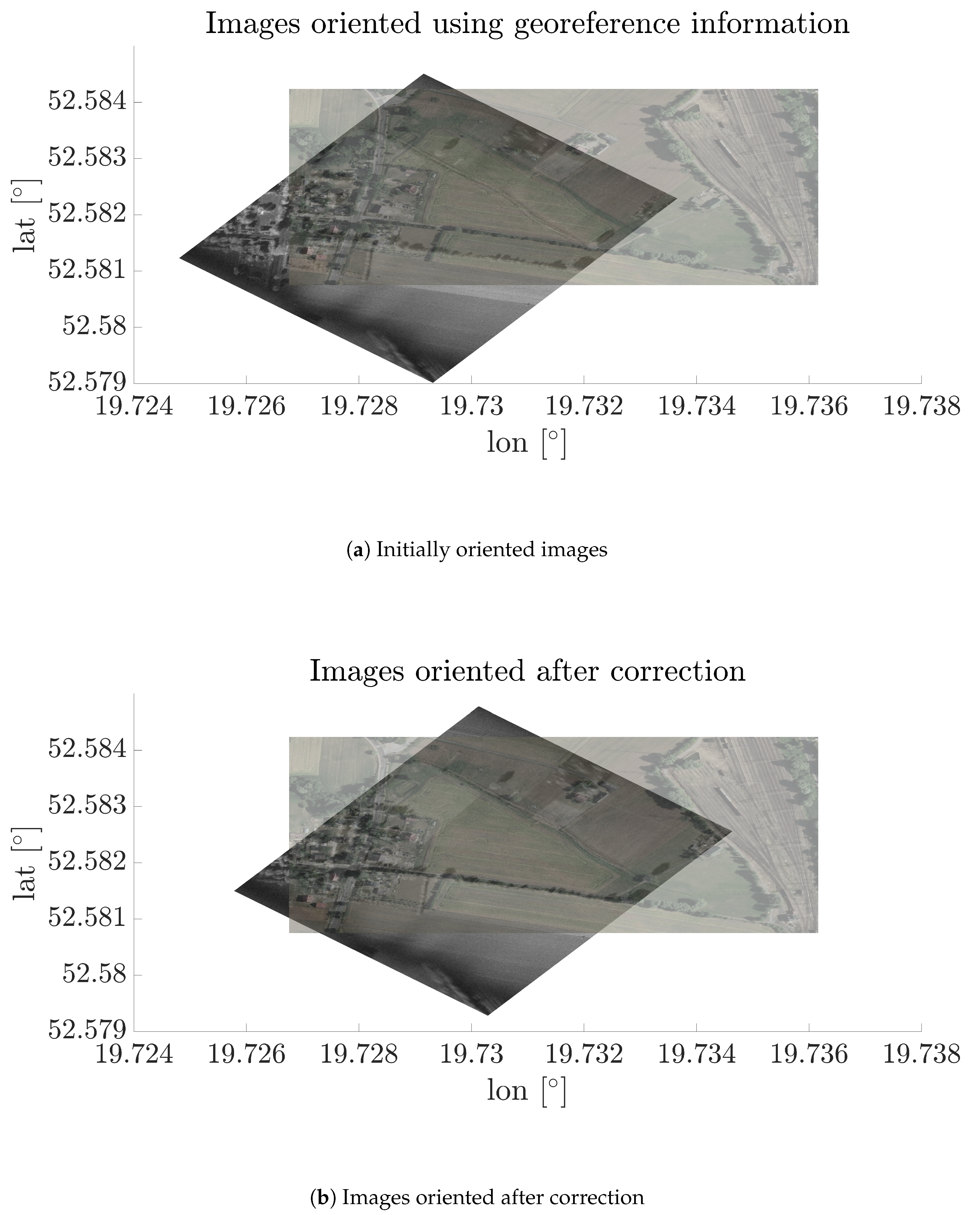
- The orientation accuracy of marked check-points.
- Generation of the SAR raster with georeferences based on the trajectory information.This step is one of the most important parts in the whole automatic registration process. It influences both the computation time and convergence of the ICP process.
- Pre-processing of SAR data to reduce the influence of the noise.
- RAW data
- Multilook-2D filter
- Averaging filter
- Minimum Mean Square Error filter
- Enhanced Lee filter
- Gamma MAP filter
- SAR Block Matching 3D filter
- Selection of the part of the orthophotomap which approximately covers the SAR image, based on the SAR footprint extended by 50 m in each direction.
- Detection and matching of the keypoints using the modified ASIFT algorithms in the SAR images and orthophotomaps:
- 4.1.
- Detection of keypoints in RAW SAR images on three pyramid levels (full resolutions, as well as 1/2, 1/4, and 1/16 of the full resolution of the raster)—ASIFT algorithm.
- 4.2.
- Detection of keypoints in SAR images with the speckle noise reduction parameters: 1, 4, 8, and 16 levels (full resolution, and 1/2, 1/4, and 1/16 of the full resolution of the raster)—ASIFT algorithm.
- 4.3.
- Detection of keypoints on orthophotomap levels (full resolution, as well as 1/2, 1/4, and 1/16 of the full resolution of the raster)—ASIFT algorithm.
- 4.4.
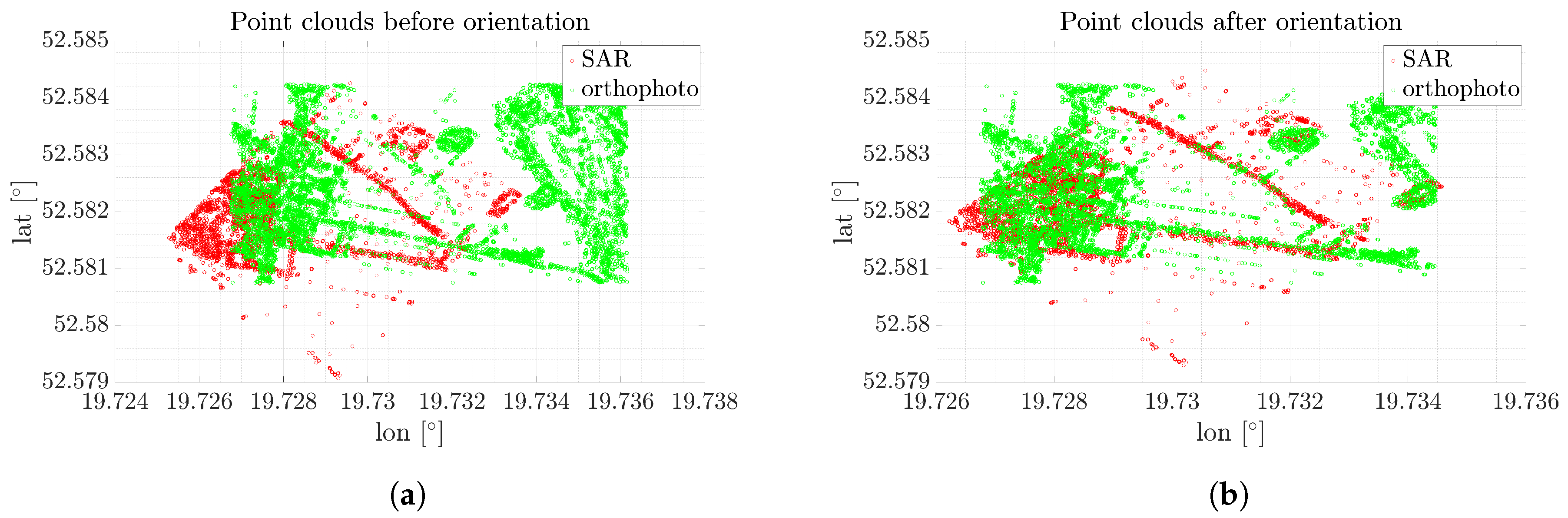
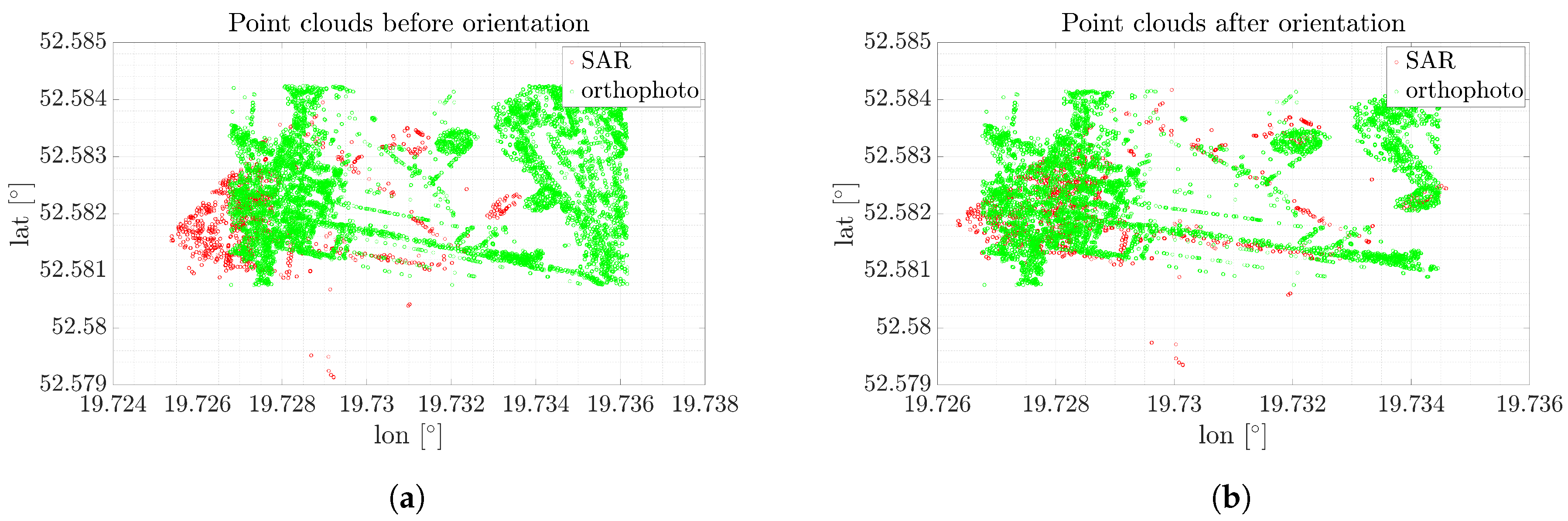
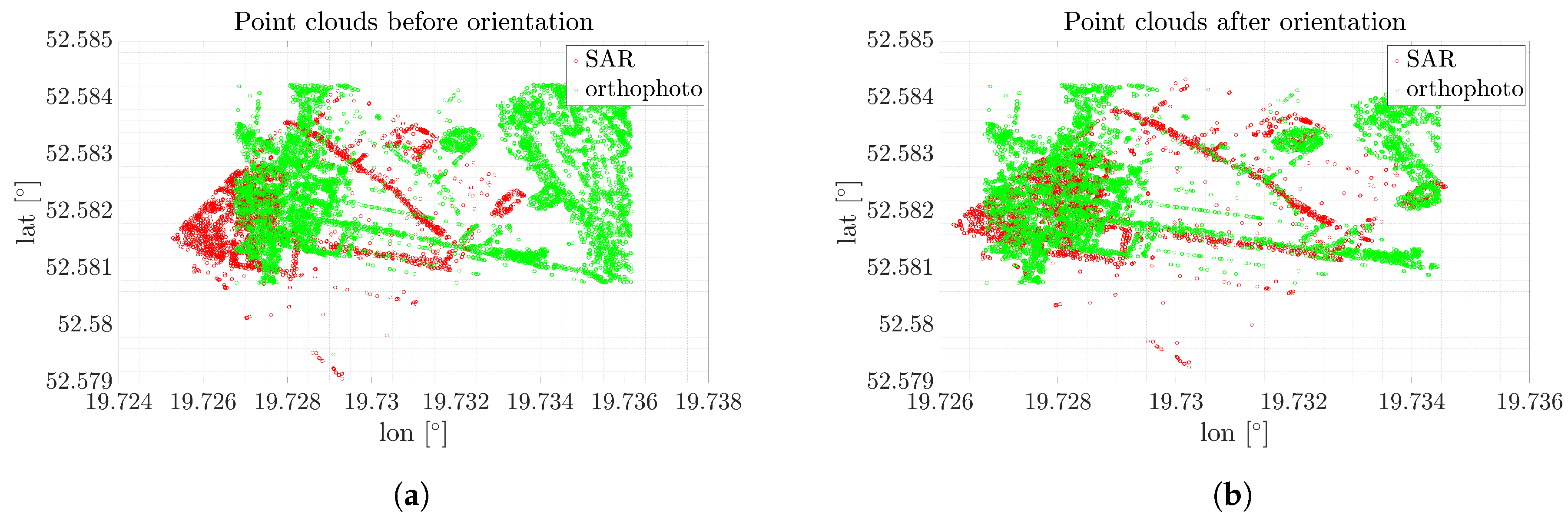
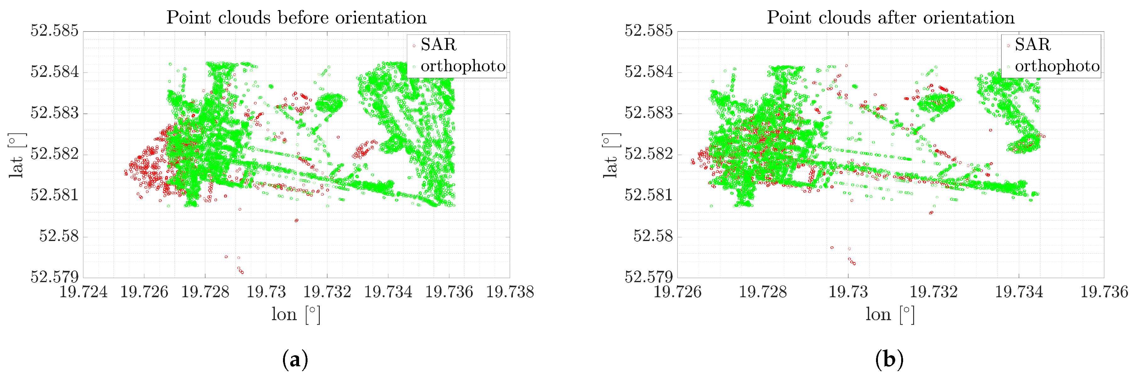
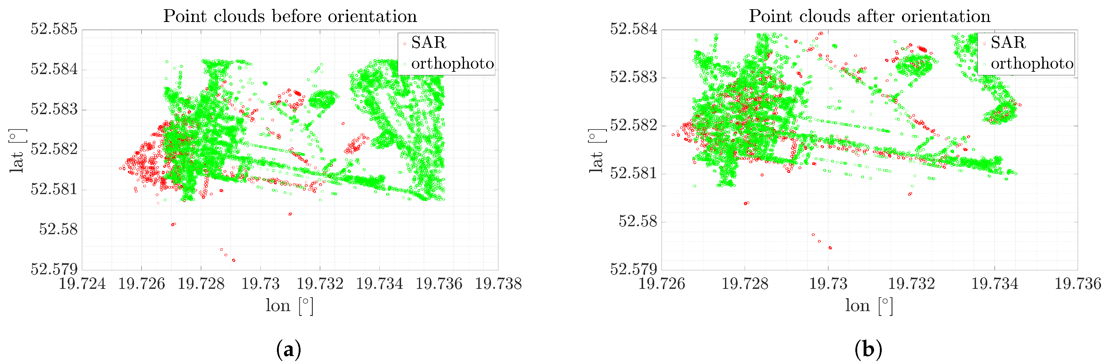
- Matching keypoints by the incremental ICP method:
- Approximate registration with 20 iterations and linear threshold deviation 20 m.
- Removal of orthophotomap keypoints that are outside the SAR area.
- Registration with 10 iterations and linear threshold deviation 5 m.
- Removal of the SAR point outliers based on the .
- Final bundle adjustment.
- Analysis of the quality of data registration on the marked check-points.
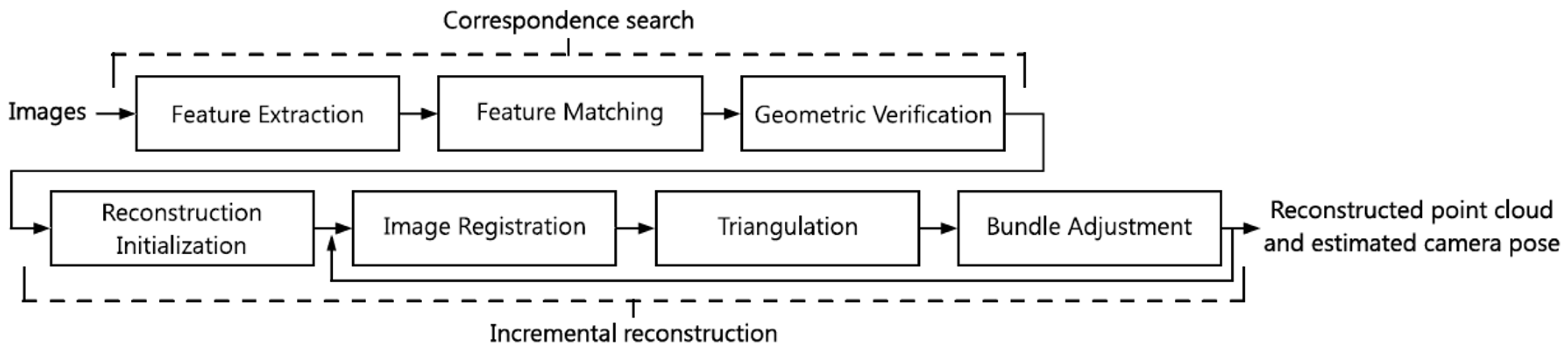
3. The Principles of the Structure from Motion
3.1. The Feature Extraction
3.2. The Feature Description
3.3. The Feature Matching and Images Registration
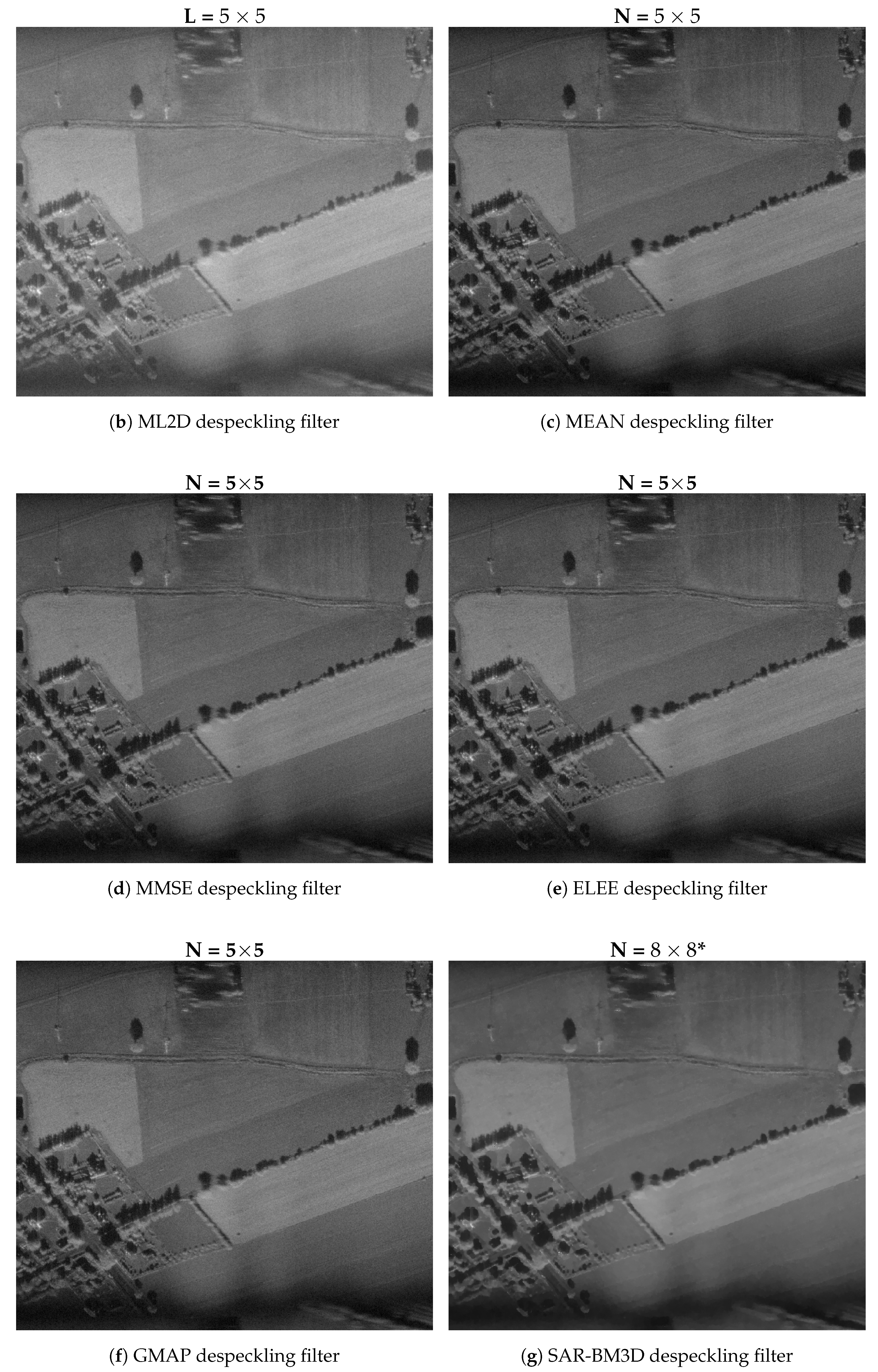
4. SAR Image Preprocessing
4.1. ML2D: Multilook–2D Filter
4.2. MEAN: Averaging Filter
4.3. MMSE: Minimum Mean Square Error Filter
4.4. ELEE: Enhanced Lee Filter
4.5. GMAP: Gamma MAP Filter
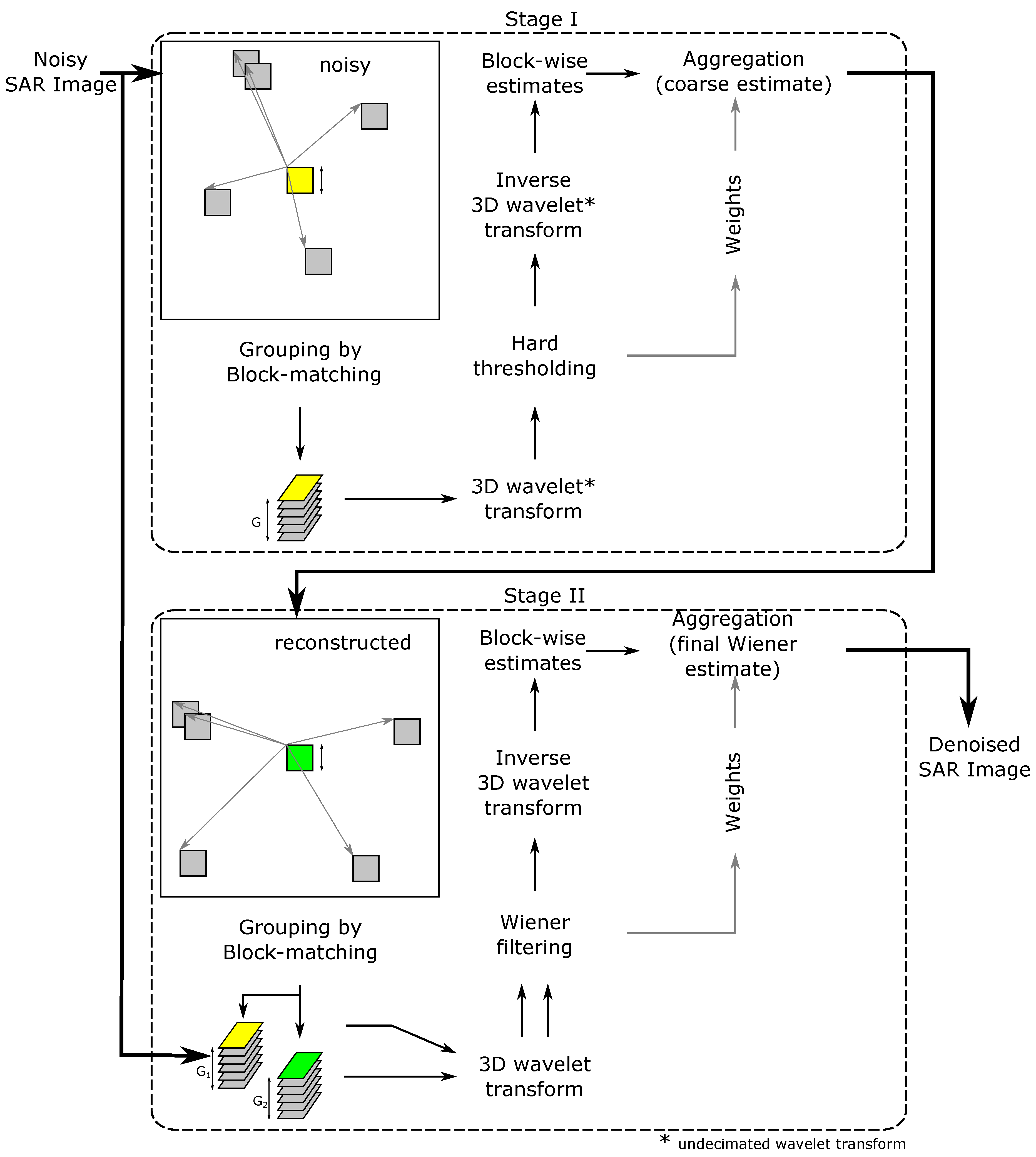
4.6. SAR-BM3D: SAR Block Matching 3D Filter
- grouping—for each reference block, the most similar blocks are grouped together;
- collaborative filtering—each 3D group undergoes UWT(Undecimated Wavelet Transformation); hard thresholding, and inverse UWT; and
- aggregation—all filtered blocks are suitably weighted, giving a coarse estimate of the image.
- grouping—blocks are located based on the coarse estimate provided by the first stage;
- collaborative filtering—each 3D group (of noisy blocks) undergoes WT((Decimated) Wavelet Transformation); Wiener filtering, and inverse WT; and
- aggregation—as in Stage 1, giving a final estimate of the image.
4.7. Filtration Performance
5. Results
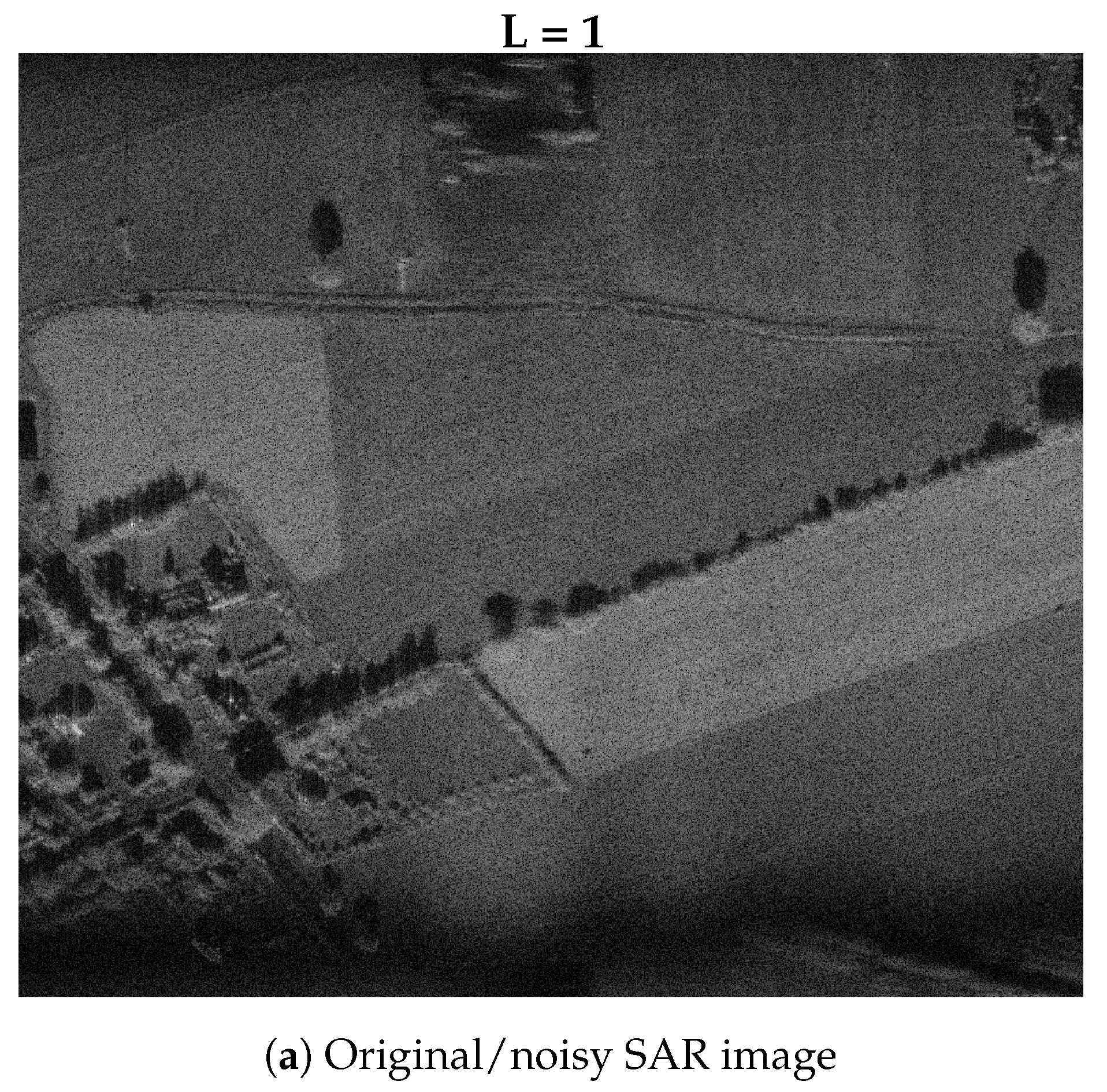
5.1. Original SAR Image
5.2. SAR Image Filtered Using ML2D
5.3. SAR Image Filtered Using MEAN Filter
5.4. SAR Image Filtered Using MMSE Filter
5.5. SAR Image Filtered Using ELEE Filter
5.6. SAR Image Filtered Using GMAP Filter
5.7. SAR Image Filtered Using SAR-BM3D Filter
5.8. Discussion
6. Conclusions
- filter SAR images;
- find keypoints on SAR and optical images;
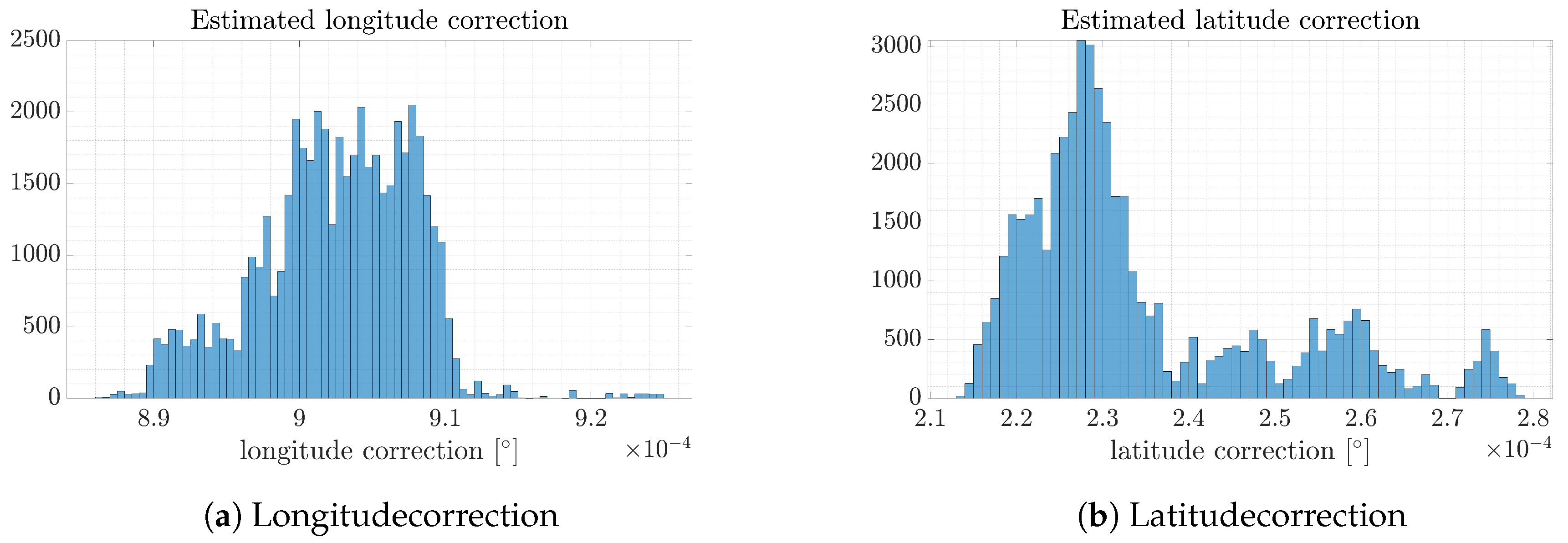
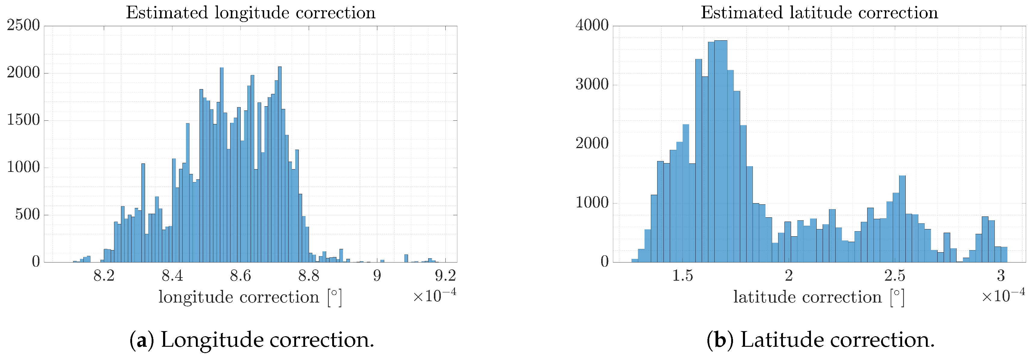
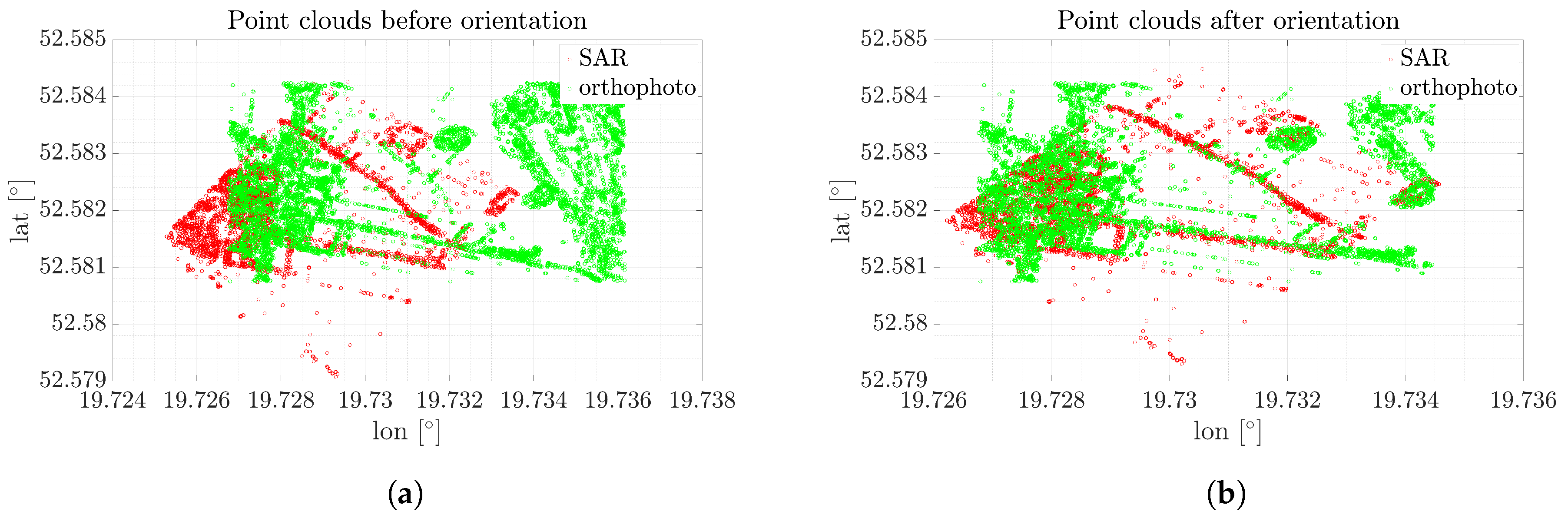
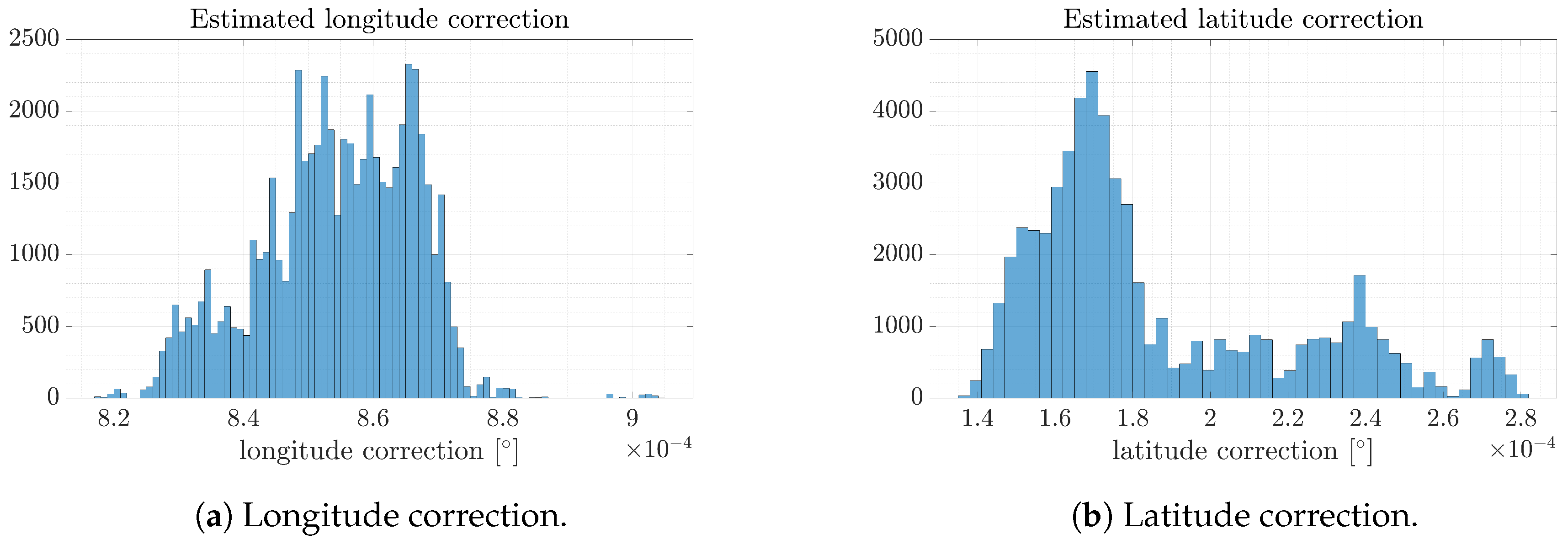
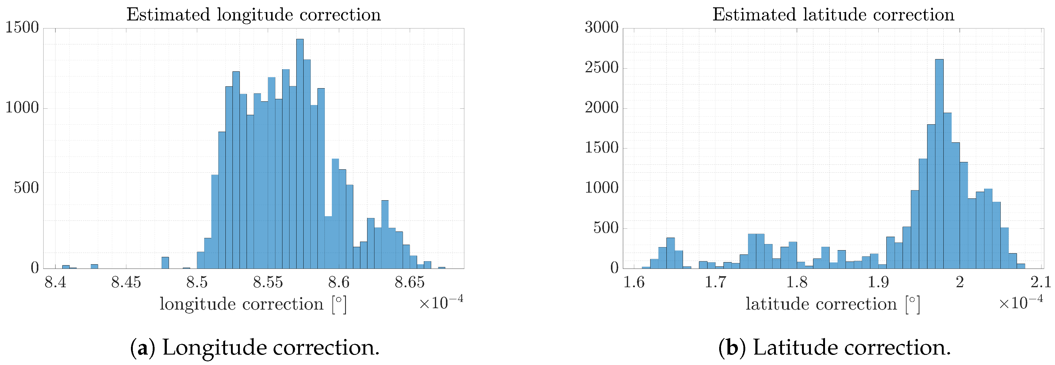
- find shift and rotation correction between images; and
- calculate navigation correction between an acquired SAR image and a reference optical image.
Author Contributions
Funding
Conflicts of Interest
Appendix A
Appendix A.1. Figures for SAR Image Filtered Using MEAN filter


Appendix A.2. Figures for SAR Image Filtered Using MMSE Filter


Appendix A.3. Figures for SAR Image Filtered Using ELEE Filter


Appendix A.4. Figures for SAR Image Filtered Using GMAP Filter


Appendix A.5. Figures for SAR Image Filtered Using SAR-BM3D Filter


References
- Golden, P.J. Terrain contour matching (TERCOM): A cruise missile guidance aid. Image Process. Missile Guid. 1980, 238, 10–18. [Google Scholar] [CrossRef]
- Vaman, D. TERRAIN REFERENCED NAVIGATION: History, trends and the unused potential. In Proceedings of the 31st Digital Avionics Systems, Williamsburg, VA, USA, 14–18 October 2012; pp. 1–28. [Google Scholar]
- Hwang, Y.; Tahk, M.J. Terrain Referenced UAV Navigation With LIDAR—A Comparison of Sequential Processing and Batch Processing Algorithms. In Proceedings of the 28th International Congress of the Aeronautical Sciences, ISAC, Brisbane, Australia, 23–28 September 2012; pp. 1–7. [Google Scholar]
- Greco, M.; Pineli, G.; Kulpa, K.; Samczyński, P.; Querry, B.; Querry, S. The study on SAR images exploitation for air platform navigation purposes. In Proceedings of the International Radar Symposium (IRS 2011), Leipzig, Germany, 7–9 September 2011; pp. 347–352. [Google Scholar]
- Greco, M.; Kulpa, K.; Pinelli, G.; Samczyński, P. SAR and InSAR georeferencing algorithms for Inertial Navigations Systems. In Proceedings of the SPIE, Bellingham, WA, USA, 7 October 2011. [Google Scholar]
- Greco, M.; Querry, S.; Pinelli, G.; Kulpa, K.; Samczyński, P.; Gromek, D.; Gromek, A.; Malanowski, M.; Querry, B.; Bonsignore, A. SAR-based Augmented Integrity Navigation Architecture. In Proceedings of the IRS 2012, Warsaw, Poland, 23–25 May 2012; pp. 225–229. [Google Scholar]
- Abratkiewicz, K.; Gromek, D.; Samczyński, P.; Markiewicz, J.; Ostrowski, W. The Concept of Applying a SIFT Algorithm and Orthophotomaps in SAR-based Augmented Integrity Navigation Systems. In Proceedings of the 2019 20th International Radar Symposium (IRS), Ulm, Germany, 26–28 June 2019; pp. 1–12. [Google Scholar]
- Gromek, D.; Samczyński, P.; Abratkiewicz, K.; Drozdowicz, J.; Radecki, K.; Stasiak, K. System Architecture for a Miniaturized X-band SAR-based Navigation Aid System. In Proceedings of the 2019 Signal Processing Symposium (SPSympo), Krakow, Poland, 17–19 September 2019; pp. 271–276. [Google Scholar] [CrossRef]
- Salehpour, M.; Behrad, A. Hierarchical approach for synthetic aperture radar and optical image coregistration using local and global geometric relationship of invariant features. J. Appl. Remote Sens. 2017, 11, 015002. [Google Scholar] [CrossRef]
- Schmitt, M.; Tupin, F.; Zhu, X.X.; Saclay, P. FUSION OF SAR AND OPTICAL REMOTE SENSING DATA—CHALLENGES AND RECENT TRENDS Signal Processing in Earth Observation; Technical University of Munich (TUM): Munich, Germany, 2017; pp. 5458–5461. [Google Scholar]
- He, C.; Fang, P.; Xiong, D.; Wang, W.; Liao, M. A point pattern chamfer registration of optical and SAR images based on mesh grids. Remote Sens. 2018, 10, 1837. [Google Scholar] [CrossRef]
- Wang, B.; Zhang, J.; Lu, L.; Huang, G.; Zhao, Z. A Uniform SIFT-Like Algorithm for SAR Image Registration. IEEE Geosci. Remote Sens. Lett. 2015, 12, 1426–1430. [Google Scholar] [CrossRef]
- Costantini, M.; Zavagli, M.; Martin, J.; Medina, A.; Barghini, A.; Naya, J.; Hernando, C.; Macina, F.; Ruiz, I.; Nicolas, E.; et al. Automatic coregistration of SAR and optical images exploiting complementary geometry and mutual information. Int. Geosci. Remote Sens. Symp. 2018, 2018, 8877–8880. [Google Scholar]
- Kai, L.; Xueqing, Z. Review of research on registration of sar and optical remote sensing image based on feature. In Proceedings of the 2018 IEEE 3rd International Conference on Signal and Image Processing (ICSIP), Shenzhen, China, 13–15 July 2018; pp. 111–115. [Google Scholar]
- Liu, F.; Bi, F.; Chen, L.; Shi, H.; Liu, W. Feature-Area Optimization: A Novel SAR Image Registration Method. IEEE Geosci. Remote Sens. Lett. 2016, 13, 242–246. [Google Scholar] [CrossRef]
- Zhang, H.; Li, G.; Lin, H. An automatic co-registration approach for optical and SAR data in urban areas. Ann. GIS 2016, 22, 235–243. [Google Scholar] [CrossRef]
- Hellwich, O.; Wefelscheid, C.; Lukaszewicz, J.; Hänsch, R.; Siddique, M.A.; Stanski, A. Integrated matching and geocoding of SAR and optical satellite images. Lect. Notes Comput. Sci. 2013, 7887, 798–807. [Google Scholar]
- Fan, B.; Huo, C.; Pan, C.; Kong, Q. Registration of optical and sar satellite images by exploring the spatial relationship of the improved SIFT. IEEE Geosci. Remote Sens. Lett. 2013, 10, 657–661. [Google Scholar] [CrossRef]
- Dellinger, F.; Delon, J.; Gousseau, Y.; Michel, J.; Tupin, F. SAR-SIFT: A SIFT-like algorithm for applications on SAR images. IEEE Trans. Geosci. Remote Sens. 2012, 3478–3481. [Google Scholar] [CrossRef]
- Bianco, S.; Ciocca, G.; Marelli, D. Evaluating the Performance of Structure from Motion Pipelines. J. Imaging 2018, 4, 98. [Google Scholar] [CrossRef]
- Saurer, O.; Fraundorfer, F.; Pollefeys, M. OmniTour: Semi-automatic generation of interactive virtual tours from omnidirectional video. In Proceedings of the 3DPVT (Int. Symp. on 3D Data Processing, Visualization and Transmission) Espace Saint Martin, Paris, France, 17–20 May 2010. [Google Scholar]
- Noh, Z.; Sunar, M.S.; Pan, Z. A review on augmented reality for virtual heritage system. In Lecture Notes in Computer Science (Including Subseries Lecture Notes in Artificial Intelligence and Lecture Notes in Bioinformatics); Springer: Berlin/Heidelberg, Germany, 2009. [Google Scholar]
- Hatzopoulos, J.N.; Stefanakis, D.; Georgopoulos, A.; Tapinaki, S.; Pantelis, V.; Liritzis, I. Use of various surveying technologies to 3D digital mapping and modelling of cultural heritage structures for maintenance and restoration purposes: The Tholos in Delphi. Greece Mediterr. Archaeol. Archaeom. 2017, 17, 311–336. [Google Scholar] [CrossRef]
- Luhmann, T.; Robson, S.; Kyle, S.; Boehm, J. Close-Range Photogrammetry and 3D Imaging; De Gruyter: Berlin, Germany; Boston, MA, USA, November 2013; ISBN 9783110302783. [Google Scholar]
- Remondino, F. IMAGE-BASED 3D MODELLING: A REVIEW. Photogramm. Rec. 2006, 21, 269–291. [Google Scholar] [CrossRef]
- Schindler, K. Developments in Computer Vision and its Relation to Photogrammetry. In Proceedings of the XXII ISPRS Congress, Melbourne, Australia, 25 August–1 September 2012. [Google Scholar]
- Friedt, J. Photogrammetric 3D Structure Reconstruction Using Micmac Basics of SfM Getting Started: Picture Acquisition Methods. 2014, pp. 1–28. Available online: http://jmfriedt.free.fr/lm_sfm_eng.pdf (accessed on 9 December 2019).
- Apollonio, F.I.; Ballabeni, A.; Gaiani, M.; Remondino, F. Evaluation of feature-based methods for automated network orientation. Int. Arch. Photogramm. Remote Sens. Spat. Inf. Sci.—ISPRS Arch. 2014, 40, 47–54. [Google Scholar] [CrossRef]
- Westoby, M.J.; Brasington, J.; Glasser, N.F.; Hambrey, M.J.; Reynolds, J.M. “Structure-from-Motion” photogrammetry: A low-cost, effective tool for geoscience applications. Geomorphology 2012. [Google Scholar] [CrossRef]
- Markiewicz, J. The use of computer vision algorithms for automatic orientation of terrestrial laser scanning data. Int. Arch. Photogramm. Remote Sens. Spat. Inf. Sci.—ISPRS Arch. 2016, 41, 315–322. [Google Scholar] [CrossRef]
- Moussa, W.; Abdel-Wahab, M.; Fritsch, D. an Automatic Procedure for Combining Digital Images and Laser Scanner Data. ISPRS—Int. Arch. Photogramm. Remote Sens. Spat. Inf. Sci. 2012, XXXIX-B5, 229–234. [Google Scholar] [CrossRef]
- Moussa, W. Integration of Digital Photogrammetry and Terrestrial Laser Scanning for Cultural Heritage Data Recording. Ph.D. Thesis, University of Stuttgart, Stuttgart, Germany, 2014. [Google Scholar]
- Harris, C.; Stephens, M. A Combined Corner and Edge Detector. Proc. Alvey Vis. Conf. 1988, 1988, 23.1–23.6. [Google Scholar] [CrossRef]
- Lowe, D.G. Distinctive image features from scale-invariant keypoints. Int. J. Comput. Vis. 2004, 60, 91–110. [Google Scholar] [CrossRef]
- Bay, H.; Tuytelaars, T.; Van Gool, L. SURF: Speeded up robust features. Lect. Notes Comput. Sci. 2006, 3951, 404–417. [Google Scholar] [CrossRef]
- Cyganek, B.; Siebert, J.P. An Introduction to 3D Computer Vision Techniques and Algorithms; Wiley and Sons Ltd.: West Sussex, UK, 2009; ISBN 9780470017043. [Google Scholar]
- Bay, H.; Ess, A. Speeded-Up Robust Features (SURF). Comput. Vis. Image Understanding 2008, 110, 346–359. [Google Scholar] [CrossRef]
- Yu, G.; Morel, J.-M. ASIFT: An Algorithm for Fully Affine Invariant Comparison. Image Process. Line 2011, 1, 11–38. [Google Scholar] [CrossRef]
- Schmitt, M.; Tupin, F.; Zhu, X.X. Fusion of SAR and optical remote sensing data—Challenges and recent trends. In Proceedings of the International Geoscience and Remote Sensing Symposium (IGARSS), Fort Worth, TX, USA, 23–28 July 2017. [Google Scholar]
- Lowe, D.G. Object recognition from local scale-invariant features. Proc. Seventh IEEE Int. Conf. Comput. Vis. 1999, 2, 1150–1157. [Google Scholar] [CrossRef]
- Liu, J.; Yu, X. Research on SAR image matching technology based on SIFT. Available online: https://www.isprs.org/proceedings/XXXVII/congress/1_pdf/67.pdf (accessed on 9 December 2019).
- Tola, E.; Lepetit, V.; Fua, P. DAISY: An efficient dense descriptor applied to wide-baseline stereo. IEEE Trans. Pattern Anal. Mach. Intell. 2010, 32, 815–830. [Google Scholar] [CrossRef] [PubMed]
- Tran, T.T.H.; Marchand, E. Real-time keypoints matching: Application to visual serving. Proc.—IEEE Int. Conf. Robot. Autom. 2007, 3787–3792. [Google Scholar] [CrossRef]
- Besl, P.; McKay, N. A Method for Registration of 3-D Shapes. IEEE Trans. Pattern Anal. Mach. Intell. 1992, 14, 239–256. [Google Scholar] [CrossRef]
- PCL PCL. Available online: http://www.pointclouds.org/downloads/ (accessed on 24 July 2019).
- VTK VTK. Available online: https://vtk.org/ (accessed on 24 July 2019).
- Open3D Open3D. Available online: http://www.open3d.org/ (accessed on 24 July 2019).
- Theiler, P.W.; Schindler, K. Automatic Registration of Terrestrial Laser Scanner Point Clouds Using Natural Planar Surfaces. ISPRS Ann. Photogr. Remote Sens. Spat. Inf. Sci. 2012, 3, 173–178. [Google Scholar] [CrossRef]
- Liu, Y. Automatic registration of overlapping 3D point clouds using closest points. Image Vis. Comput. 2006, 24, 762–781. [Google Scholar] [CrossRef]
- Bae, K.H.; Lichti, D.D. A method for automated registration of unorganised point clouds. ISPRS J. Photogramm. Remote Sens. 2008, 63, 36–54. [Google Scholar] [CrossRef]
- Sprickerhof, J.; Nüchter, A.; Lingemann, K.; Hertzberg, J. An Explicit Loop Closing Technique for 6D SLAM. In Proceedings of the 4th European Conference on Mobile Robots, Dubrovnik, Croatia, 23–25 September 2009; pp. 1–6. [Google Scholar]
- Vosselman, G.; Maas, H.-G. Airborne and Terrestrial Laser Scanning. Current 2010, XXXVI, 318. [Google Scholar]
- Arun, K.S.; Huang, T.S.; Blostein, S.D. Least-Squares Fitting of Two 3-D Point Sets. IEEE Trans. Pattern Anal. Mach. Intell. 1987, 9, 698–700. [Google Scholar] [CrossRef] [PubMed]
- Horn, B.K.P. Closed-form solution of absolute orientation using unit quaternions. J. Opt. Soc. Am. A 1987, 4, 629. [Google Scholar] [CrossRef]
- Horn, B.; Hilden, P.K.; Hugh, M.; Shahriar, N. Closed-form solution of absolute orientation using orthonormal matrices. J. Opt. Soc. Am. A 1988, 5, 1127. [Google Scholar] [CrossRef]
- Walker, M.W.; Shao, L.; Volz, R.A. Estimating 3-D location parameters using dual number quaternions. CVGIP Image Underst. 1991, 54, 358–367. [Google Scholar] [CrossRef]
- Eggert, D.W.; Lorusso, A.; Fisher, R.B. Estimating 3-D rigid body transformations: A comparison of four major algorithms. Mach. Vis. Appl. 1997, 9, 272–290. [Google Scholar] [CrossRef]
- Fischler, M.A.; Bolles, R.C. Random sample consensus: A paradigm for model fitting with applications to image analysis and automated cartography. Commun. ACM 1981. [Google Scholar] [CrossRef]
- Torr, P.H.S.; Zisserman, A. MLESAC: A new robust estimator with application to estimating image geometry. Comput. Vis. Image Underst. 2000, 78, 138–156. [Google Scholar] [CrossRef]
- Oliver, C.; Quegan, S. Understanding Synthetic Aperture Radar Images; SciTech Radar and Defense Series; SciTech Publ.: Raleigh, NC, USA, 2004; ISBN 1891121316. [Google Scholar]
- Gromek, A. SAR Imagery Non-Coherent Change Detection Methods. Ph.D. Dissertation, Warsaw Univ. of Tech. Publ., Warsaw, PL, USA, July 2019. [Google Scholar]
- Jakowatz, C.V.; Wahl, D.E.; Eichel, P.H.; Ghiglia, D.C.; Thompson, P.A. Spotlight-Mode Synthetic Aperture Radar: A Signal Processing Approach; Kluwer Academic Publ.: Norwell, MA, USA, 1996; pp. 105–218. ISBN 0792396774. [Google Scholar]
- Scott, R. Maximum Likelihood Estimation: Logic and Practice; SAGE Publ.: Newbury Park, CA, USA, 1993; pp. 46–56. ISBN 0803941072. [Google Scholar]
- Lee, J.S. Refined filtering of image noise using local statistics. Comp. Graph. Image Proc. 1981, 15, 380–390. [Google Scholar] [CrossRef]
- Lee, J.S. A simple speckle smoothing algorithm for synthetic aperture radar images. I3E Trans. Syst. Man Cybern. 1983, 13, 85–89. [Google Scholar] [CrossRef]
- Jakeman, E. On the statistics of K-distributed noise. J. Phys. A Math. Gen. 1980, 13, 31. [Google Scholar] [CrossRef]
- Frost, V.S. A model for radar images and its application to adaptive filtering of multiplicative noise. I3E Trans. Pattern Anal. Machine Intell. 1982, 4, 157–166. [Google Scholar] [CrossRef] [PubMed]
- Kuan, D.T. Adaptive restoration of images with speckle. I3E Trans. Acoust. Speech Signal Process. 1987, 35, 373–383. [Google Scholar] [CrossRef]
- Lopes, A. Structure detection and adaptive speckle filtering in SAR images. Int. J. Remote Sens. 1993, 14. [Google Scholar] [CrossRef]
- Poderico, M. Denoising of SAR Image. Ph.D. Thesis, University of Naples Federico II, Naples, IT, USA, November 2011. [Google Scholar]


| Filter Type | ENL\ENIL | Processing Time |
|---|---|---|
| Ml2d | 23.9 | 12 s |
| Mean | 21.7 | 23 s |
| Mmse | 17.9 | 43 s |
| Elee | 19.3 | 03 m:25 s |
| Gmap | 24.1 | 03 m:28 s |
| Sar-Bm3d | 199.2 | 04 h:05 m:17 s |
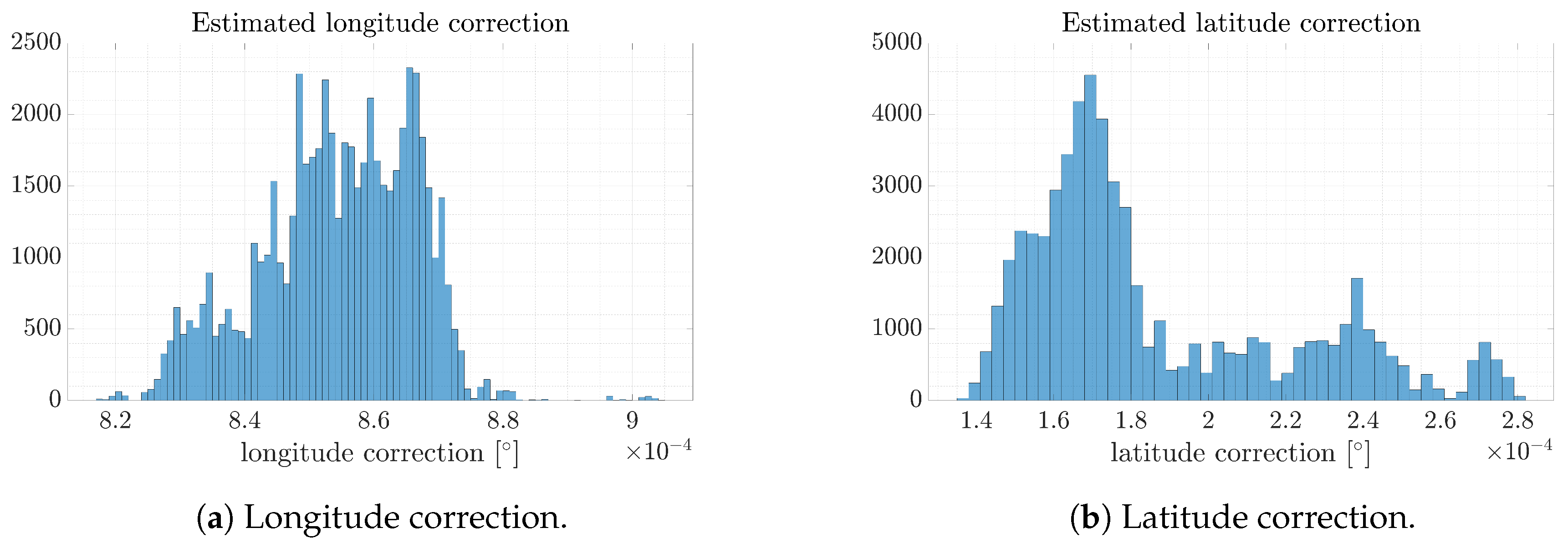
| Filter Type | Longitude Correction | Latitude Correction | Rotation | Processing Time [s] | Amount of Keypoints |
|---|---|---|---|---|---|
| No filter | 4.0919 | 111.7241 | 367,584 | ||
| ML2D | 0.9416 | 79.9240 | 49,153 | ||
| MEAN | 0.5612 | 71.8246 | 65,489 | ||
| MMSE | 0.6804 | 77.3086 | 66,917 | ||
| ELEE | 1.2547 | 71.1760 | 58,165 | ||
| GMAP | 0.0051 | 66.2229 | 22,200 | ||
| BM3D | 0.3204 | 66.9932 | 24,954 |
© 2019 by the authors. Licensee MDPI, Basel, Switzerland. This article is an open access article distributed under the terms and conditions of the Creative Commons Attribution (CC BY) license (http://creativecommons.org/licenses/by/4.0/).
Share and Cite
Markiewicz, J.; Abratkiewicz, K.; Gromek, A.; Ostrowski, W.; Samczyński, P.; Gromek, D. Geometrical Matching of SAR and Optical Images Utilizing ASIFT Features for SAR-based Navigation Aided Systems. Sensors 2019, 19, 5500. https://doi.org/10.3390/s19245500
Markiewicz J, Abratkiewicz K, Gromek A, Ostrowski W, Samczyński P, Gromek D. Geometrical Matching of SAR and Optical Images Utilizing ASIFT Features for SAR-based Navigation Aided Systems. Sensors. 2019; 19(24):5500. https://doi.org/10.3390/s19245500
Chicago/Turabian StyleMarkiewicz, Jakub, Karol Abratkiewicz, Artur Gromek, Wojciech Ostrowski, Piotr Samczyński, and Damian Gromek. 2019. "Geometrical Matching of SAR and Optical Images Utilizing ASIFT Features for SAR-based Navigation Aided Systems" Sensors 19, no. 24: 5500. https://doi.org/10.3390/s19245500
APA StyleMarkiewicz, J., Abratkiewicz, K., Gromek, A., Ostrowski, W., Samczyński, P., & Gromek, D. (2019). Geometrical Matching of SAR and Optical Images Utilizing ASIFT Features for SAR-based Navigation Aided Systems. Sensors, 19(24), 5500. https://doi.org/10.3390/s19245500