Stress Estimation Using Digital Image Correlation with Compensation of Camera Motion-Induced Error


Abstract
1. Introduction
2. Residual Stress Estimation
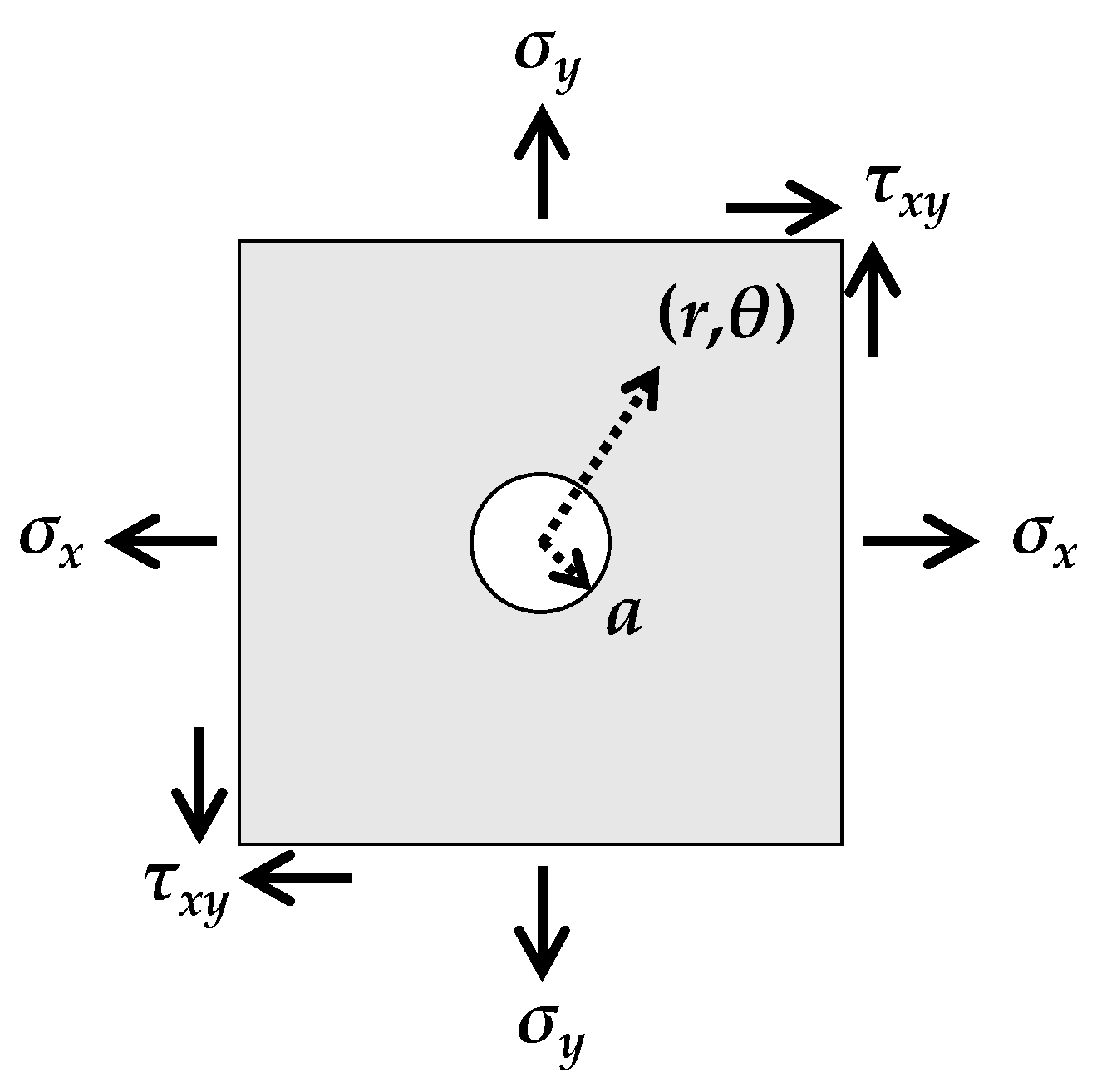
2.1. Residual Stress Estimation
2.2. Residual Stress Estimation with Camera Motion-Induced Error
3. Camera Motion-Independent Residual Stress Estimation
3.1. Extraction of Homography-Independent Component
3.2. Residual Stress Estimation Using the Homography-Independent Terms
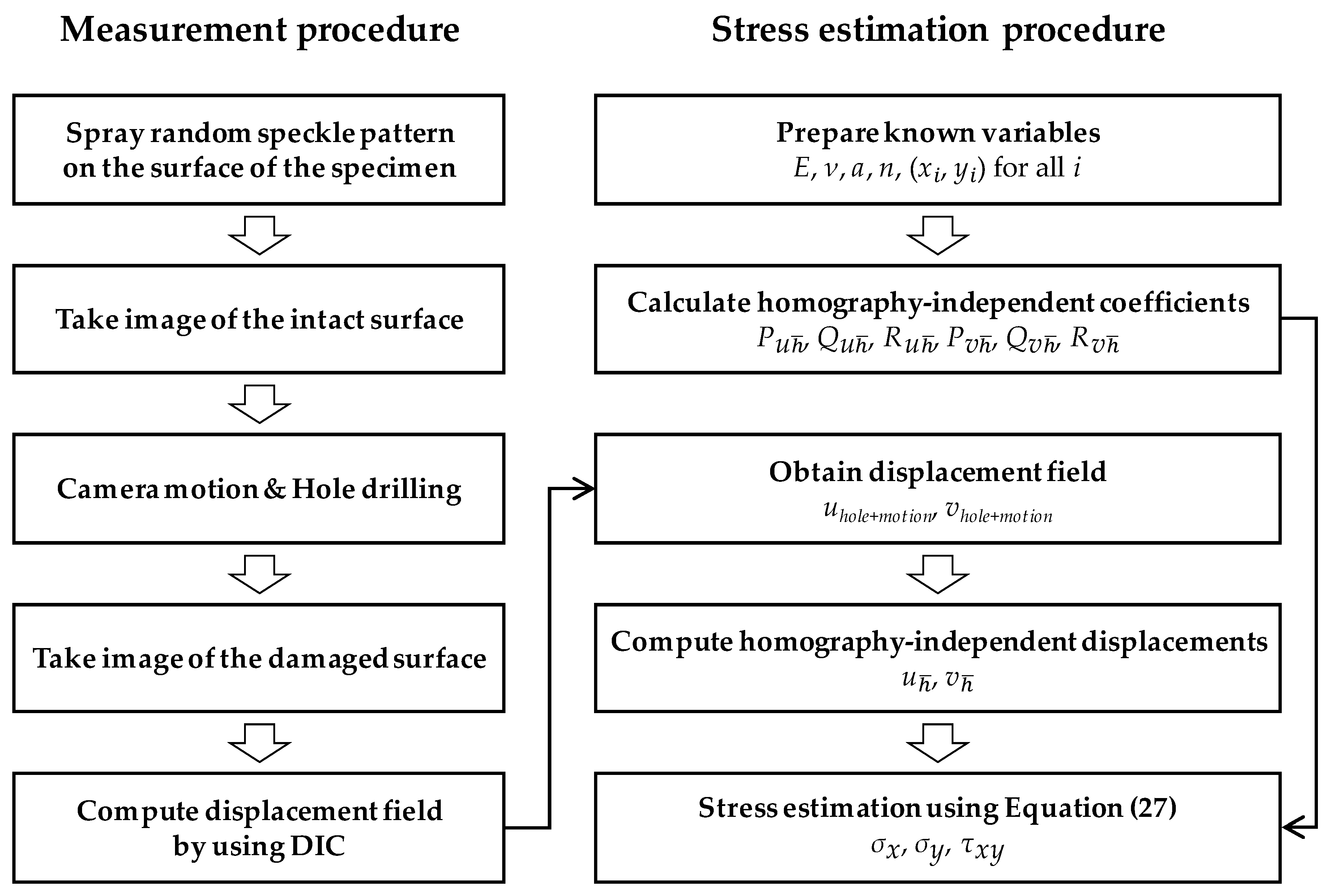
3.3. Summary of the Proposed Method
- E, ν, a, n, x, and y are given before the measurement based on the material properties, hole-drilling scheme, and image resolution.
- Derive , , , , , and using the given E, ν, a, n, x, and y (known at step 1) based on Equation (2)–(10).
- Derive , , , , , and by numerically generating multiple pairs of displacement fields (uh, vh) and residual stresses (σx, σy, τxy) based on Equations (31) and (32).
- Derive , , , , , and by subtracting , , , , , and (derived at step 3), respectively from , , ,, , and (derived at step 2) based on Equation (25).
- Obtain the displacement field uhole+motion and vhole+motion by applying DIC to the images of before and after the hole drill engaged with camera motion.
- Compute H in Equation (22) by using correspondences between {x, y} (known at step 1) and {uhole+motion, vhole+motion} (obtained at step 5) for all material points using direct linear transform [35].
- Compute and by using uhole+motion and vhole+motion (obtained at step 5) in combination with H (obtained at step 6) based on Equations (22)–(24).
- Compute the residual stresses σx, σy, and τxy using and (obtained at step 7) in combination with , , , , , and (derived at step 4) using Equation (27).
4. Numerical Validation
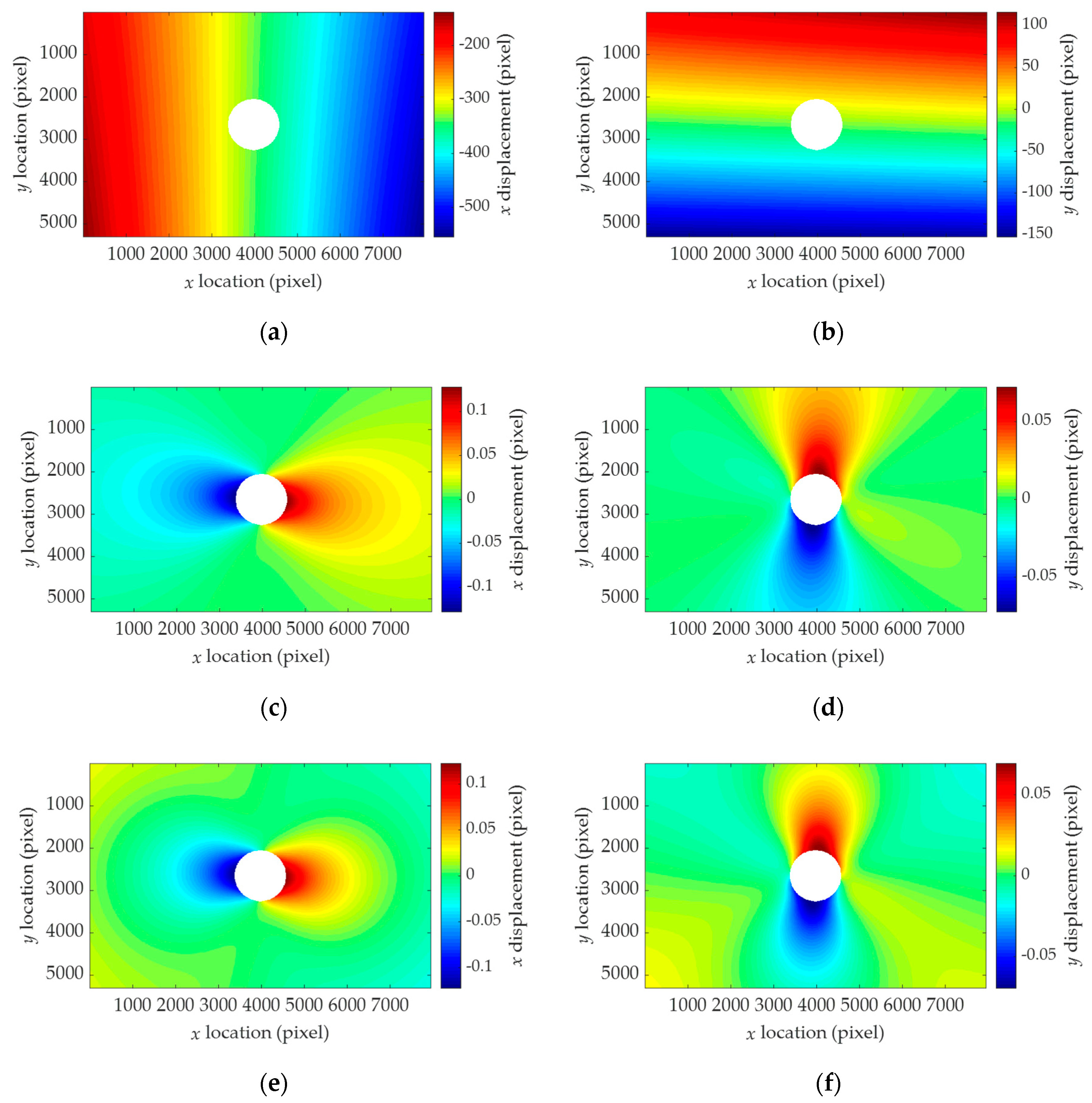
4.1. Numerical Generation of the Displacement Field
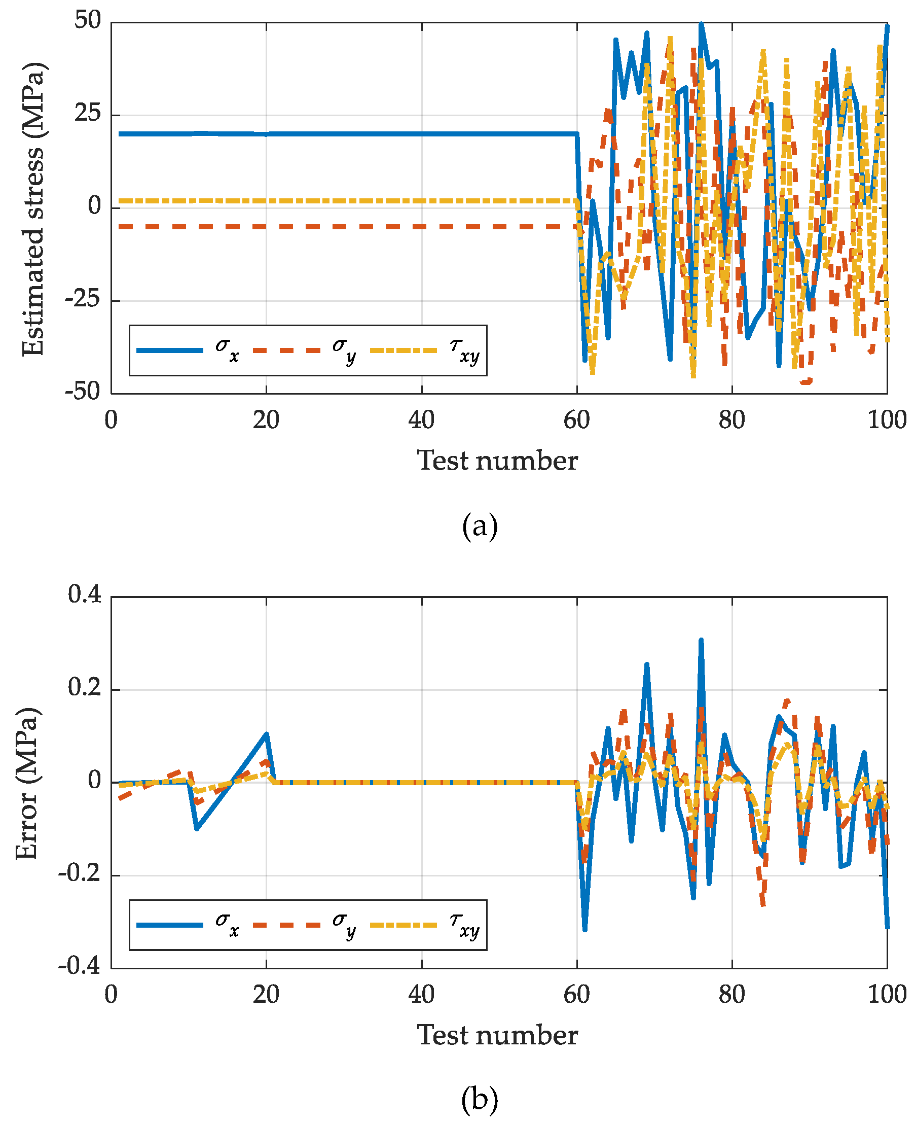
4.2. Stress Estimation Using the Proposed Method
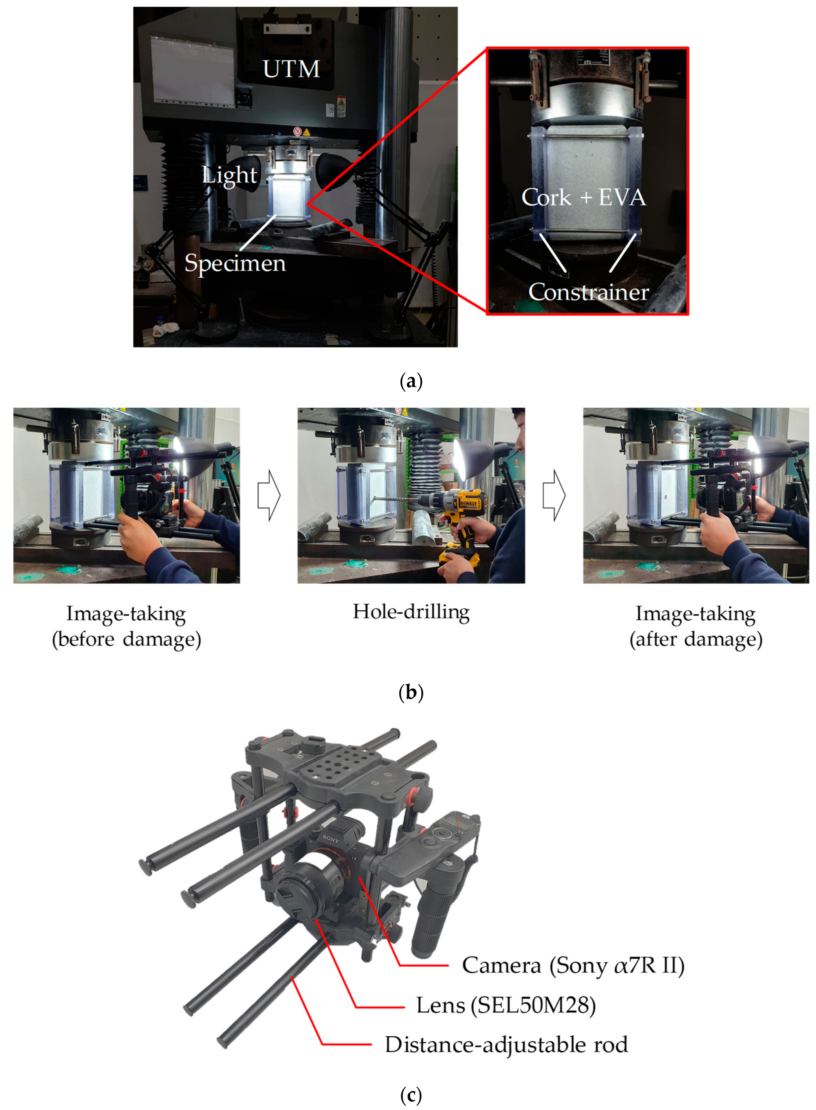
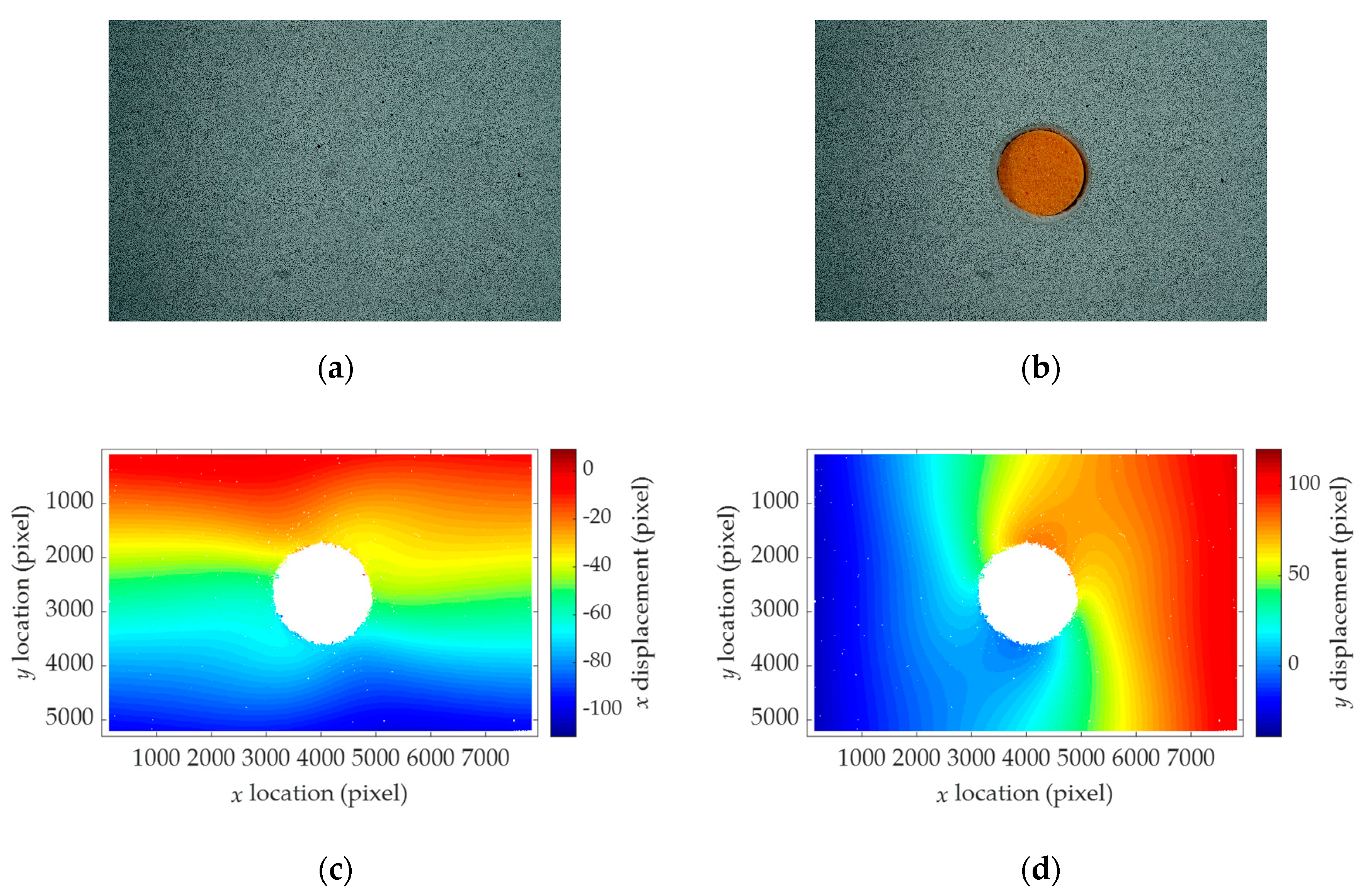
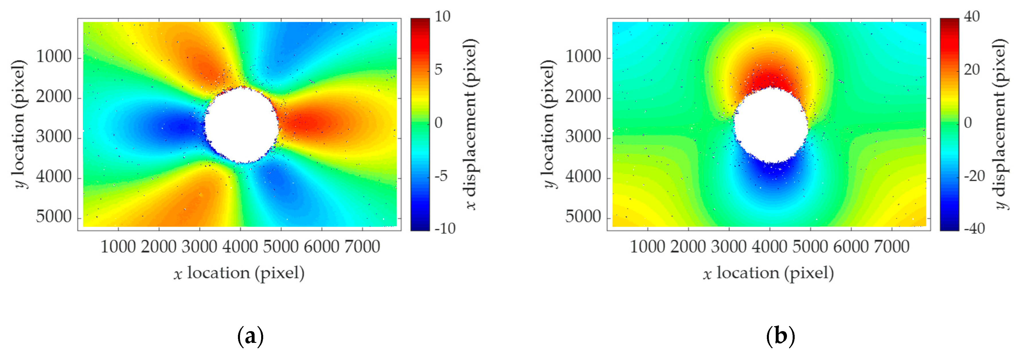
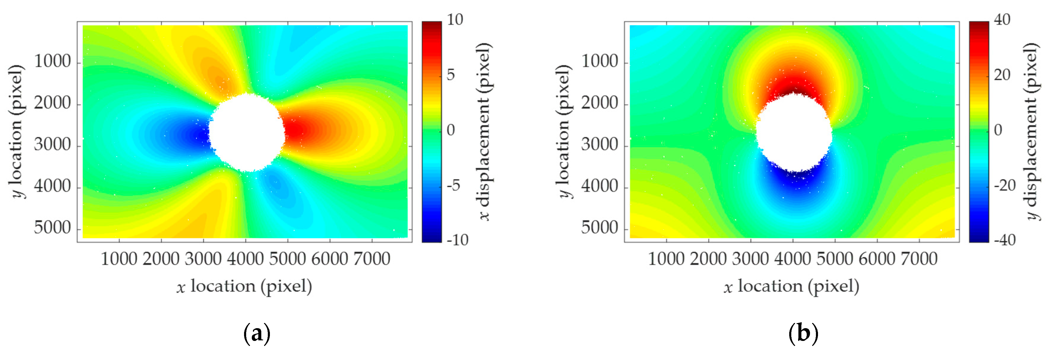
5. Laboratory-Scale Validation
6. Conclusions
Author Contributions
Funding
Conflicts of Interest
Nomenclature
| σx | In-plane residual stress (normal stress along x direction). |
| σy | In-plane residual stress (normal stress along y direction). |
| τxy | In-plane residual stress (shear stress). |
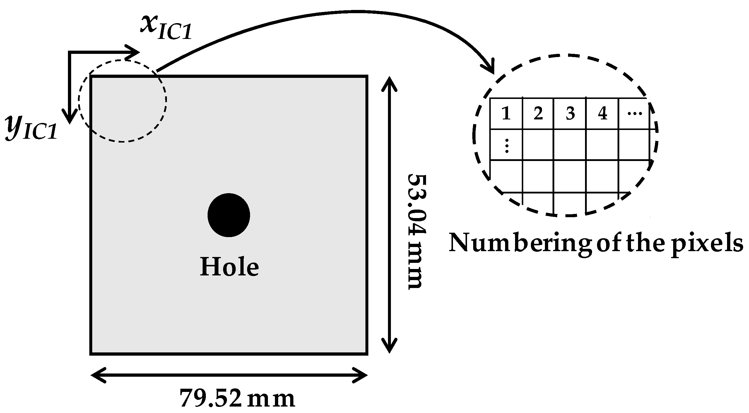
| xi | x coordinate of i-th material point. |
| yi | y coordinate of i-th material point. |
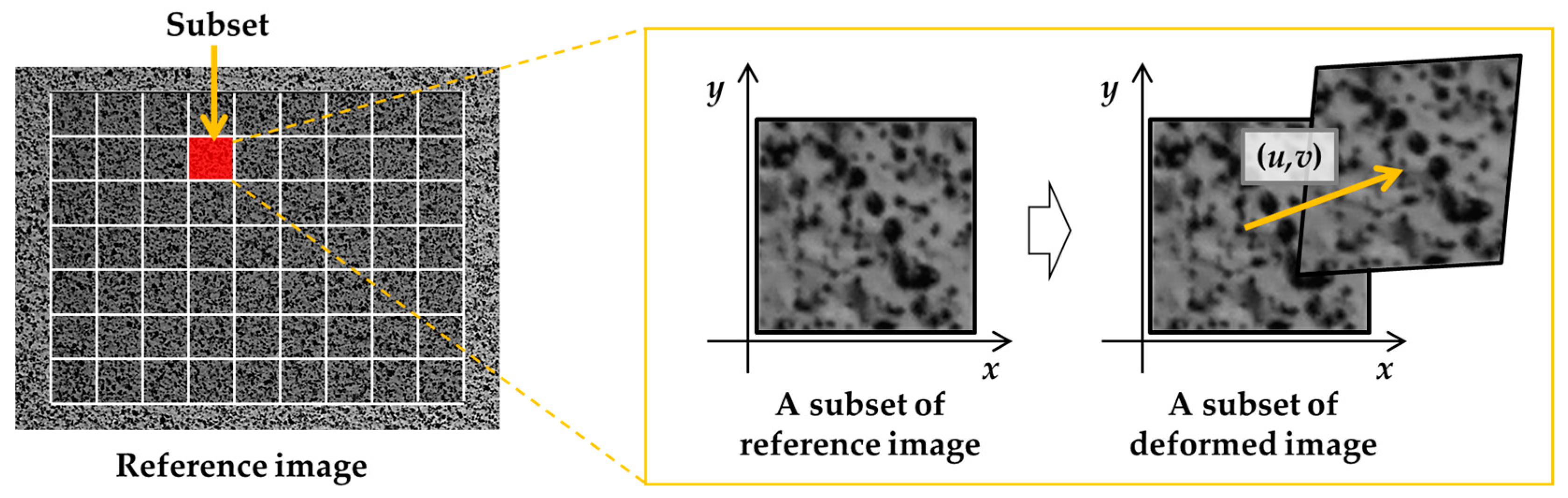
| uhole(xi, yi) | x directional displacement at {xi, yi} induced by hole-drilling. |
| vhole(xi, yi) | y directional displacement at {xi, yi} induced by hole-drilling. |
| umotion(xi, yi) | x directional displacement at {xi, yi} induced by camera motion. |
| vmotion(xi, yi) | y directional displacement at {xi, yi} induced by camera motion. |
| uhole+motion(xi, yi) | x directional displacement at {xi, yi} induced by hole-drilling and camera motion. |
| vhole+motion(xi, yi) | y directional displacement at {xi, yi} induced by hole-drilling and camera motion. |
| uh(xi, yi) | Homography-dependent x directional displacement among uhole+motion(xi, yi). |
| vh(xi, yi) | Homography-dependent y directional displacement among vhole+motion(xi, yi). |
| (xi, yi) | Homography-independent x directional displacement among uhole+motion(xi, yi). |
| (xi, yi) | Homography-independent y directional displacement among vhole+motion(xi, yi). |
| Pu | Stress coefficient for linear relationship between σx and uhole(xi, yi). |
| Qu | Stress coefficient for linear relationship between σy and uhole(xi, yi). |
| Ru | Stress coefficient for linear relationship between τxy and uhole(xi, yi). |
| Pv | Stress coefficient for linear relationship between σx and vhole(xi, yi). |
| Qv | Stress coefficient for linear relationship between σy and vhole(xi, yi). |
| Rv | Stress coefficient for linear relationship between τxy and vhole(xi, yi). |
| Puh | Stress coefficient for linear relationship between σx and uh(xi, yi). |
| Quh | Stress coefficient for linear relationship between σy and uh(xi, yi). |
| Ruh | Stress coefficient for linear relationship between τxy and uh(xi, yi). |
| Pvh | Stress coefficient for linear relationship between σx and vh(xi, yi). |
| Qvh | Stress coefficient for linear relationship between σy and vh(xi, yi). |
| Rvh | Stress coefficient for linear relationship between τxy and vh(xi, yi). |
| Stress coefficient for linear relationship between σx and (xi, yi). | |
| Stress coefficient for linear relationship between σy and (xi, yi). | |
| Stress coefficient for linear relationship between τxy and (xi, yi). | |
| Stress coefficient for linear relationship between σx and (xi, yi). | |
| Stress coefficient for linear relationship between σy and (xi, yi). | |
| Stress coefficient for linear relationship between τxy and (xi, yi). | |
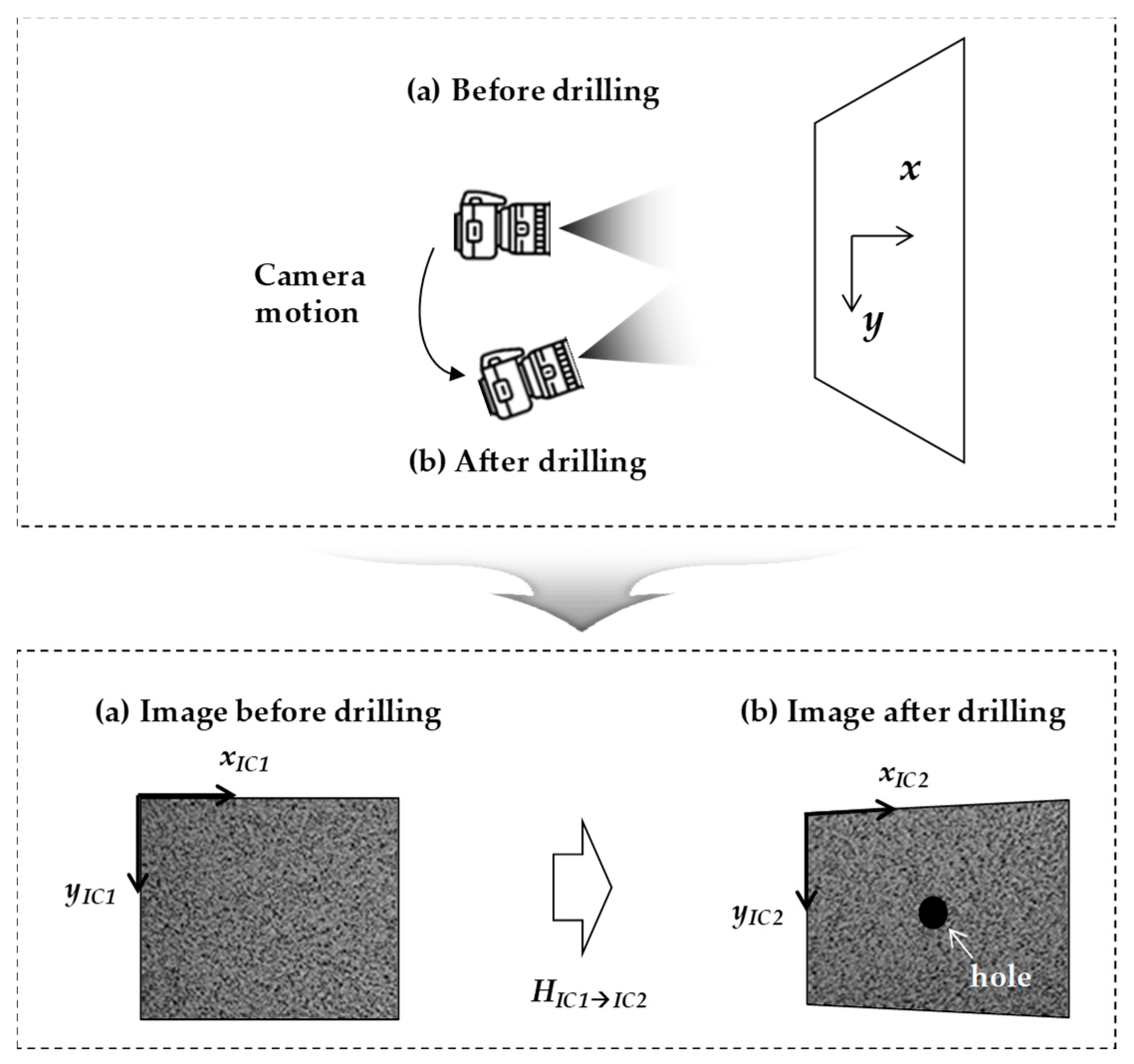
| IC1 | Image coordinate system before the hole-drilling and camera motion. |
| IC2 | Image coordinate system after the hole-drilling and camera motion. |
| s | Scaling factor that holds the third component (w) of the homogeneous representation {x, y, w}T in 1. |
| HIC1→IC2 | Homography transform from IC1 to IC2 associated with 6DOF camera motion. |
| Hh | Principal homography transform. |
| H | HIC1→IC2Hh. |
References
- Schajer, G.S. Advances in hole-drilling residual stress measurements. Exp. Mech. 2010, 50, 159–168. [Google Scholar] [CrossRef]
- Montross, C.S.; Wei, T.; Ye, L.; Clark, G.; Mai, Y.W. Laser shock processing and its effects on microstructure and properties of metal alloys: A review. Int. J. Fatigue 2002, 24, 1021–1036. [Google Scholar] [CrossRef]
- Krauss, G. Martensite in steel: Strength and structure. Mater. Sci. Eng. A Struct. Mater. Prop. Microstruct. Process. 1999, 273, 40–57. [Google Scholar] [CrossRef]
- Nilson, A.H.; Winter, G.; Urquhart, L.C.; Charles Edward, O.R. Design of Concrete Structures; McGraw-Hill: New York, NY, USA, 1991. [Google Scholar]
- Mathar, J. Determination of initial stresses by measuring the deformation around drilled holes. Trans. ASME 1934, 56, 249–254. [Google Scholar]
- Rossini, N.S.; Dassisti, M.; Benyounis, K.Y.; Olabi, A.G. Methods of measuring residual stresses in components. Mater. Des. 2012, 35, 572–588. [Google Scholar] [CrossRef]
- Schajer, G.S. Application of finite element calculations to residual stress measurements. J. Eng. Mater. Technol. 1981, 103, 157–163. [Google Scholar] [CrossRef]
- Kirsch, C. Die theorie der elastizitat und die bedurfnisse der festigkeitslehre. Z. VDI 1898, 42, 797–807. [Google Scholar]
- Nelson, D.V.; Makino, A.; Fuchs, E.A. The holographic-hole drilling method for residual stress determination. Opt. Lasers Eng. 1997, 27, 3–23. [Google Scholar] [CrossRef]
- Rendler, N.J.; Vigness, I. Hole-drilling strain-gage method of measuring residual stresses. Exp. Mech. 1966, 6, 577–586. [Google Scholar] [CrossRef]
- Beaney, E.M. Accurate measurement of residual stress on any steel using the centre hole method. Strain 1976, 12, 99–106. [Google Scholar] [CrossRef]
- Keil, S. Experimental determination of residual stresses with the ring-core method and an on-line measuring system. Exp. Tech. 1992, 16, 17–24. [Google Scholar] [CrossRef]
- Scafidi, M.; Valentini, E.; Zuccarello, B. Error and uncertainty analysis of the residual stresses computed by using the hole drilling method. Strain 2011, 47, 301–312. [Google Scholar] [CrossRef]
- Owens, A. In-situ stress determination used in structural assessment of concrete structures. Strain 1993, 29, 115–124. [Google Scholar] [CrossRef]
- Trautner, C.; McGinnis, M.J.; Pessiki, S. Application of the incremental core-drilling method to determine in-situ stresses in concrete. ACI Mater. J. 2011, 108, 290–299. [Google Scholar]
- Ruan, X.; Zhang, Y. In-situ stress identification of bridge concrete components using core-drilling method. Struct. Infrastruct. Eng. 2015, 11, 210–222. [Google Scholar] [CrossRef]
- ASTM E837-13a. Standard Test Method for Determining Residual Stresses by the Hole-Drilling Strain-Gage Method; ASTM International: West Conshohocken, PA, USA, 2013.
- Lin, S.T.; Hsieh, C.T.; Hu, C.P. Two holographic blind-hole methods for measuring residual stresses. Exp. Mech. 1994, 34, 141–147. [Google Scholar] [CrossRef]
- Min, Y.; Hong, M.; Xi, Z.; Jian, L. Determination of residual stress by use of phase shifting moire interferometry and hole-drilling method. Opt. Lasers Eng. 2006, 44, 68–79. [Google Scholar] [CrossRef]
- Nelson, D.V. Residual stress determination by hole drilling combined with optical methods. Exp. Mech. 2010, 50, 145–158. [Google Scholar] [CrossRef]
- Steinzig, M.; Takahashi, T. Residual stress measurement using the hole drilling method and laser speckle interferometry part IV: Measurement accuracy. Exp. Tech. 2003, 27, 59–63. [Google Scholar] [CrossRef]
- Schmitt, D.R.; Diallo, M.S.; Weichman, F. Quantitative determination of stress by inversion of speckle interferometer fringe patterns: Experimental laboratory tests. Geophys. J. Int. 2006, 167, 1425–1438. [Google Scholar] [CrossRef]
- Albertazzi, G.; Viotti, M.R.; Kapp, W.A. A radial in-plane DSPI interferometer using diffractive optics for residual stresses measurement. In Proceedings of the SPIE 7155, Ninth International Symposium on Laser Metrology, Singapore, 30 June–2 July 2008; p. 21. [Google Scholar]
- Caminero, M.A.; Lopez-Pedrosa, M.; Pinna, C.; Soutis, C. Damage assessment of composite structures using digital image correlation. Appl. Compos. Mater. 2014, 21, 91–106. [Google Scholar] [CrossRef]
- Caminero, M.A.; Lopez-Pedrosa, M.; Pinna, C.; Soutis, C. Damage monitoring and analysis of composite laminates with an open hole and adhesively bonded repairs using digital image correlation. Compos. Part B 2013, 53, 76–91. [Google Scholar] [CrossRef]
- Baldi, A. Residual stress measurement using hole drilling and integrated digital image correlation techniques. Exp. Mech. 2014, 54, 379–391. [Google Scholar] [CrossRef]
- McGinnis, M.J.; Pessiki, S.; Turker, H. Application of three-dimensional digital image correlation to the core-drilling method. Exp. Mech. 2005, 45, 359–367. [Google Scholar] [CrossRef]
- Trautner, C.; McGinnis, M.J.; Pessiki, S. Analytical and numerical development of the incremental core-drilling method of non-destructive determination of in-situ stresses in concrete structures. J. Strain Anal. Eng. Des. 2010, 45, 647–658. [Google Scholar] [CrossRef]
- Lee, J.; Kim, E.J.; Gwon, S.; Cho, S.; Sim, S.-H. Uniaxial static stress estimation for concrete structures using digital image correlation. Sensors 2019, 19, 319. [Google Scholar] [CrossRef]
- Pan, B.; Qian, K.; Xie, H.; Asundi, A. Two-dimensional digital image correlation for in-plane displacement and strain measurement: A review. Meas. Sci. Technol. 2009, 20, 062001. [Google Scholar] [CrossRef]
- Sutton, M.A.; Orteu, J.J.; Schreier, H. Digital image correlation (DIC). In Image Correlation for Shape, Motion and Deformation Measurements: Basic Concepts, Theory and Applications, 1st ed.; Springer Science & Business Media: New York, NY, USA, 2009. [Google Scholar]
- Beghini, M.; Bertini, L.; Raffaelli, P. Numerical analysis of plasticity effects in the hole-drilling residual stress measurement. J. Test. Eval. 1994, 22, 522–529. [Google Scholar]
- Hutchings, M.T.; Krawitz, A.D. (Eds.) Measurement of Residual and Applied Stress Using Neutron Diffraction; Springer Science & Business Media: New York, NY, USA, 2012. [Google Scholar]
- Penrose, R. A generalized inverse for matrices. Proc. Camb. Philos. Soc. 1955, 51, 406–413. [Google Scholar] [CrossRef]
- Hartley, R.; Zisserman, A. Projective geometry and transformations of 2D. In Multiple View Geometry in Computer Vision, 2nd ed.; Cambridge University Press: New York, NY, USA, 2003. [Google Scholar]
- Blaber, J.; Adair, B.; Antoniou, A. Ncorr: Open-source 2D digital image correlation Matlab software. Exp. Mech. 2015, 55, 1105–1122. [Google Scholar] [CrossRef]


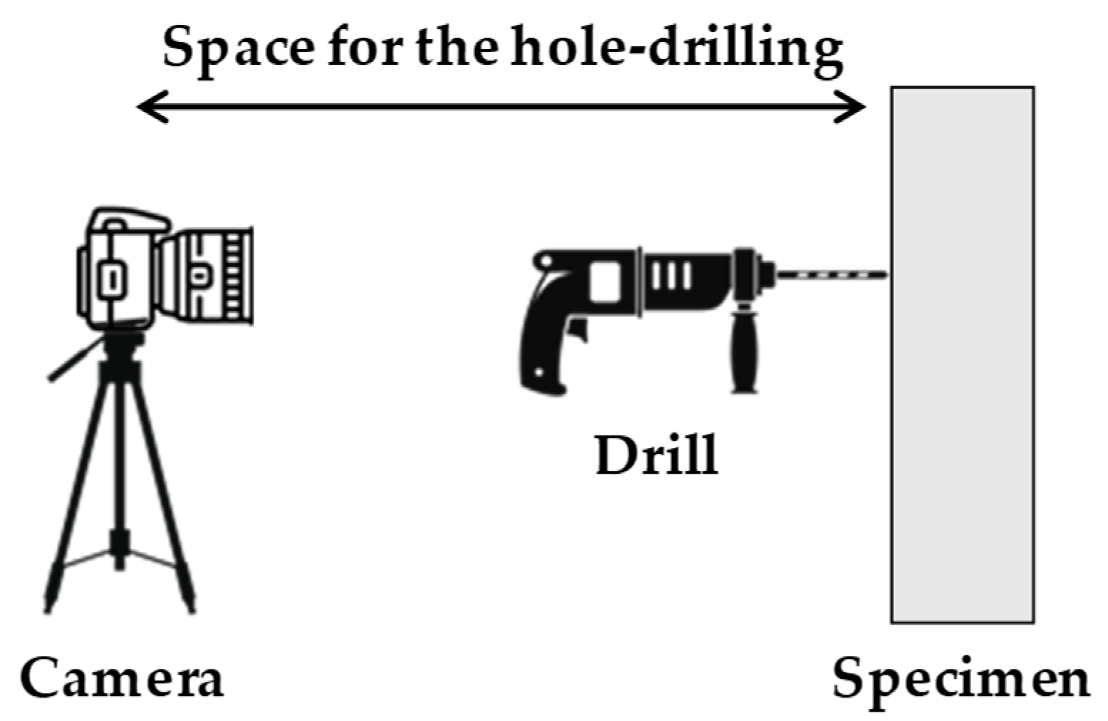
| Item | Model | Specification |
|---|---|---|
| Camera | Sony α7R II | Resolution: 7952 × 5304 pixels |
| Lens | SEL50M28 | Focal length: 50 mm |
| Test | Stress (MPa) | Camera Motions | |||||||
|---|---|---|---|---|---|---|---|---|---|
| Rotation (mrad) | Translation (mm) | ||||||||
| σx | σy | τxy | rx | ry | rz | tx | ty | tz | |
| 1–10 | 20 | −5 | 2 | [−10, 10] | 0 | 0 | 0 | 0 | 0 |
| 11–20 | 0 | [−10, 10] | 0 | 0 | 0 | 0 | |||
| 21–30 | 0 | 0 | [−10, 10] | 0 | 0 | 0 | |||
| 31–40 | 0 | 0 | 0 | [−5, 5] | 0 | 0 | |||
| 41–50 | 0 | 0 | 0 | 0 | [−5, 5] | 0 | |||
| 51–60 | 0 | 0 | 0 | 0 | 0 | [−5, 5] | |||
| 61–100 | unif(−50, 50) * | unif(−10, 10) * | unif(−5, 5) * | ||||||
| Property | Value |
|---|---|
| Young’s modulus | 2.46 MPa |
| Poisson’s ratio | 0.1 |
| Dimension (height × width × depth) | 230 × 150 × 75 mm |
| Hole diameter | 14 mm |
| Pixel resolution | 7952 × 5304 |
| Pixel density | 108.26 pixel/mm |
| Test | True stress (KPa) | Estimated Stresses (KPa) | Error (KPa) σy−σy,true | ||
|---|---|---|---|---|---|
| σy,true | σx | σy | τxy | ||
| 1 | −100.0 | −29.3 | −101.3 | +1.2 | −1.3 |
| 2 | −100.0 | −21.6 | −103.1 | −3.7 | −3.1 |
| 3 | −100.0 | −39.2 | −107.1 | −3.0 | −7.1 |
© 2019 by the authors. Licensee MDPI, Basel, Switzerland. This article is an open access article distributed under the terms and conditions of the Creative Commons Attribution (CC BY) license (http://creativecommons.org/licenses/by/4.0/).
Share and Cite
Lee, J.; Jeong, S.; Lee, Y.-J.; Sim, S.-H. Stress Estimation Using Digital Image Correlation with Compensation of Camera Motion-Induced Error. Sensors 2019, 19, 5503. https://doi.org/10.3390/s19245503
Lee J, Jeong S, Lee Y-J, Sim S-H. Stress Estimation Using Digital Image Correlation with Compensation of Camera Motion-Induced Error. Sensors. 2019; 19(24):5503. https://doi.org/10.3390/s19245503
Chicago/Turabian StyleLee, Junhwa, Seunghoo Jeong, Young-Joo Lee, and Sung-Han Sim. 2019. "Stress Estimation Using Digital Image Correlation with Compensation of Camera Motion-Induced Error" Sensors 19, no. 24: 5503. https://doi.org/10.3390/s19245503
APA StyleLee, J., Jeong, S., Lee, Y.-J., & Sim, S.-H. (2019). Stress Estimation Using Digital Image Correlation with Compensation of Camera Motion-Induced Error. Sensors, 19(24), 5503. https://doi.org/10.3390/s19245503