Leader-Following Consensus and Formation Control of VTOL-UAVs with Event-Triggered Communications †

 ,
,  , , , ,
Abstract
1. Introduction
1.1. Background and Context
1.2. Contribution of the Work
2. Preliminaries
2.1. Notation
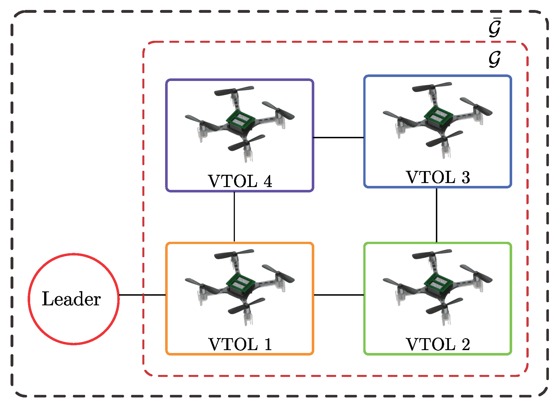
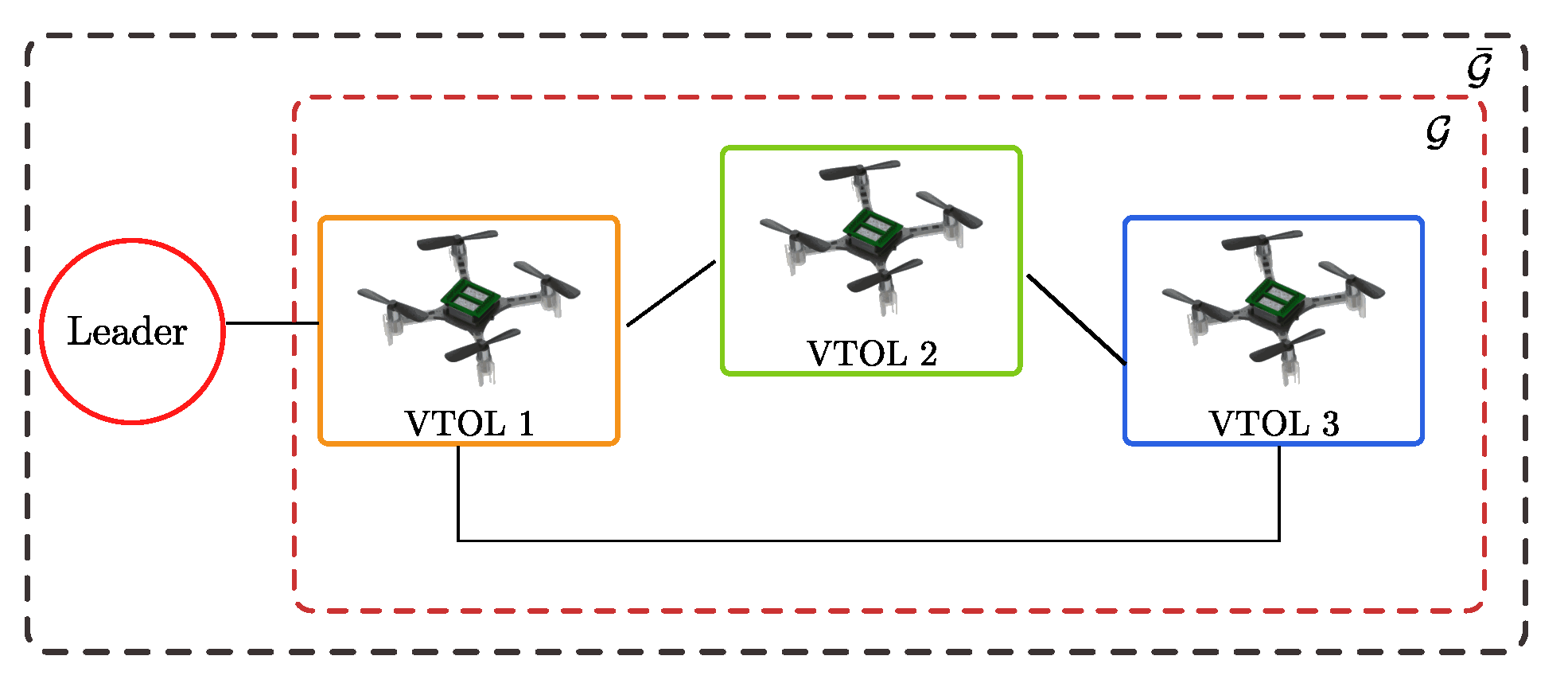
2.2. Graph Theory
- 1.
- The matrix has nonnegative eigenvalues;
- 2.
- The matrix is positive definite if and only if the graph is connected.
2.3. Dynamic Systems and Event-Triggered Communication
- An event function that pinpoints if agent i needs () or not () to transmit its state to other agents j, with where is the node i’s neighbor set. The event function for agent i depends on its current state and a memory of last time became negative.
- A (static distributed) feedback function . The feedback function takes the current state as input and memories of and of . Therefore, the control law for agent i varies with respect to (i) its current state value , (ii) its state last time an event occurred , and also (iii) the state of its neighbors last time an event occurred . The term static means the state is measured and not estimated by another dynamical system (like an observer). The term distributed means the control law for one agent i is only related to the neighbor set , which is itself a subset of the set for all nodes, i.e., .
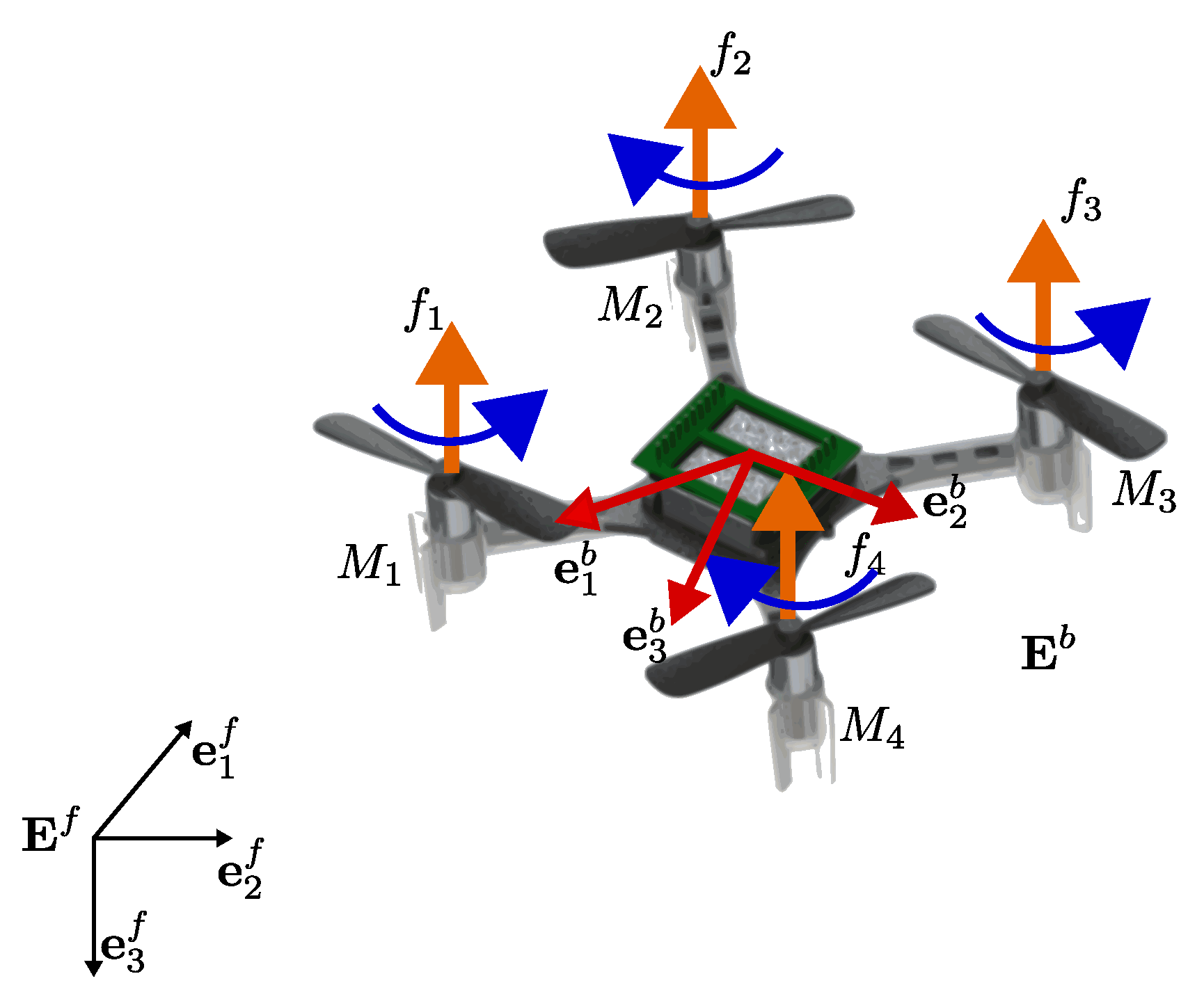
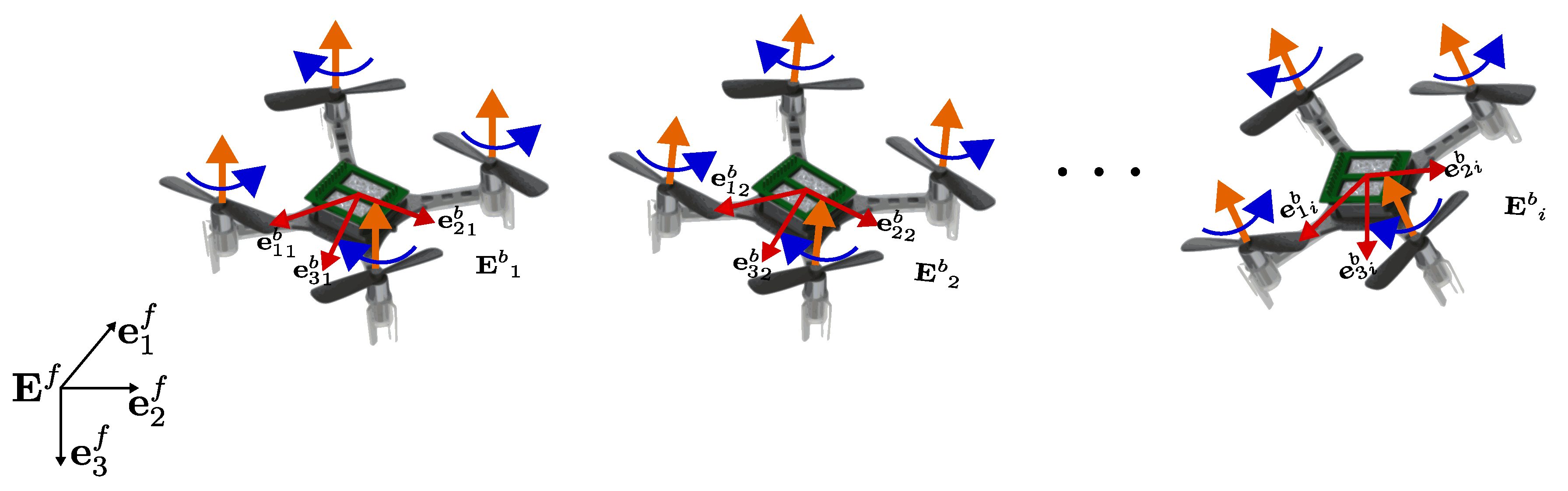
2.4. VTOL-UAV Mathematical Model
2.4.1. Attitude Representation
2.4.2. VTOL-UAVs Model
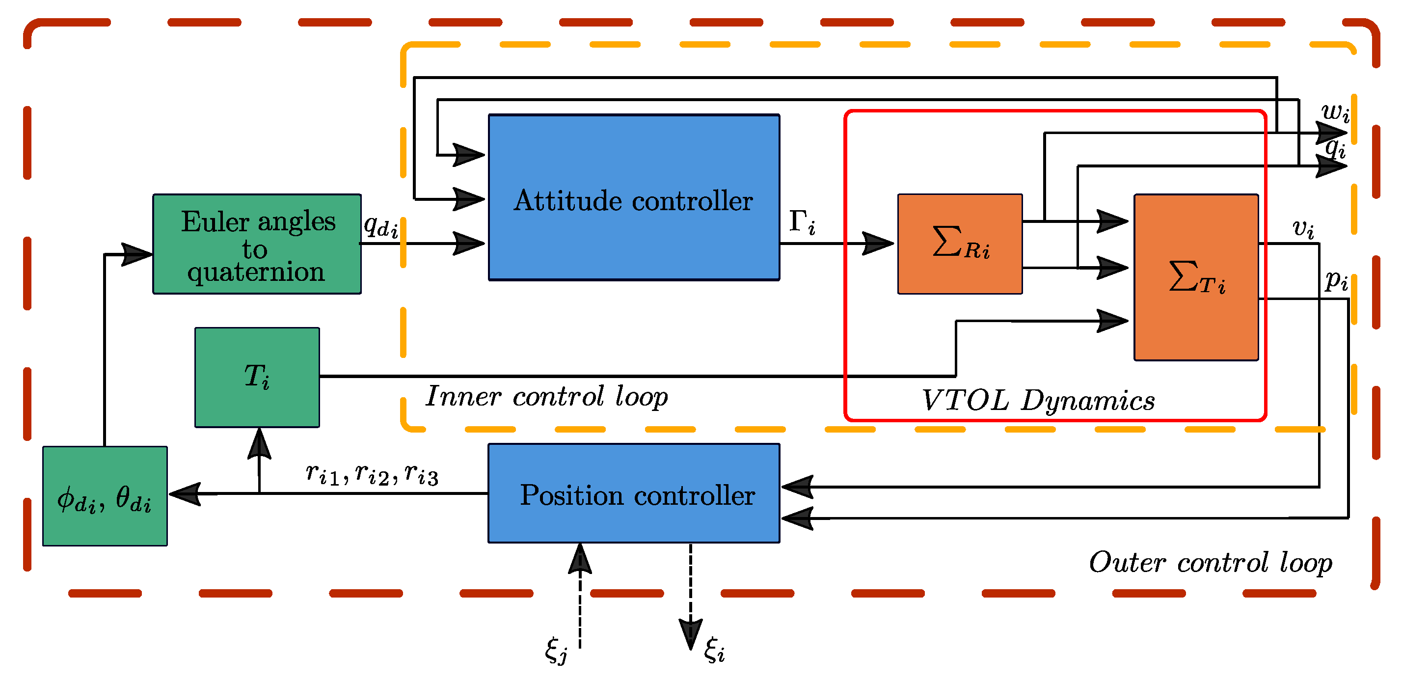
3. Attitude and Position (Inner) Control Loop
3.1. Attitude Control
3.2. Position Control
4. Distributive Event-Triggered Protocol for Consensus and Formation
4.1. Leader-Following Consensus Control
4.2. Exclusion of Zeno Behavior
4.3. Formation Control
- with
- . Note that are such that and for the unidirected graph
5. Numerical and Experimental Tests
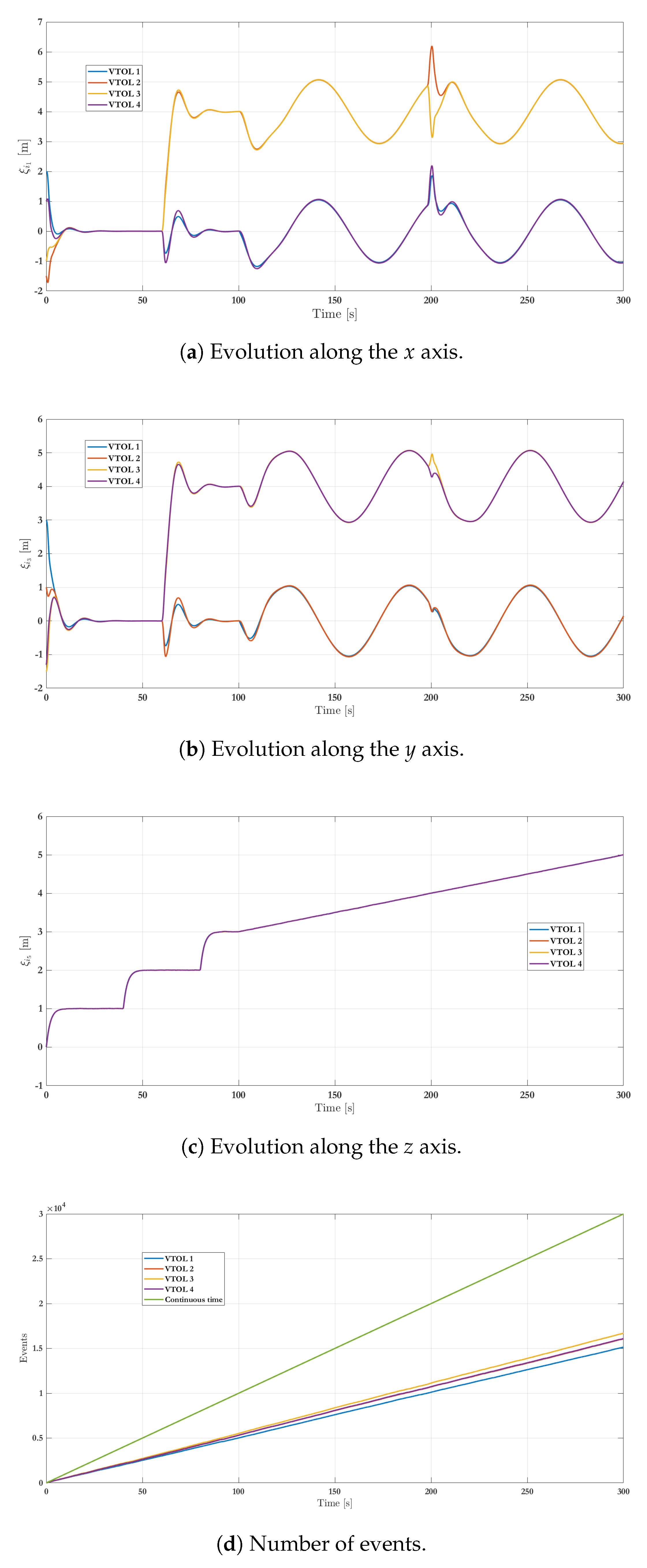
5.1. Simulation Tests
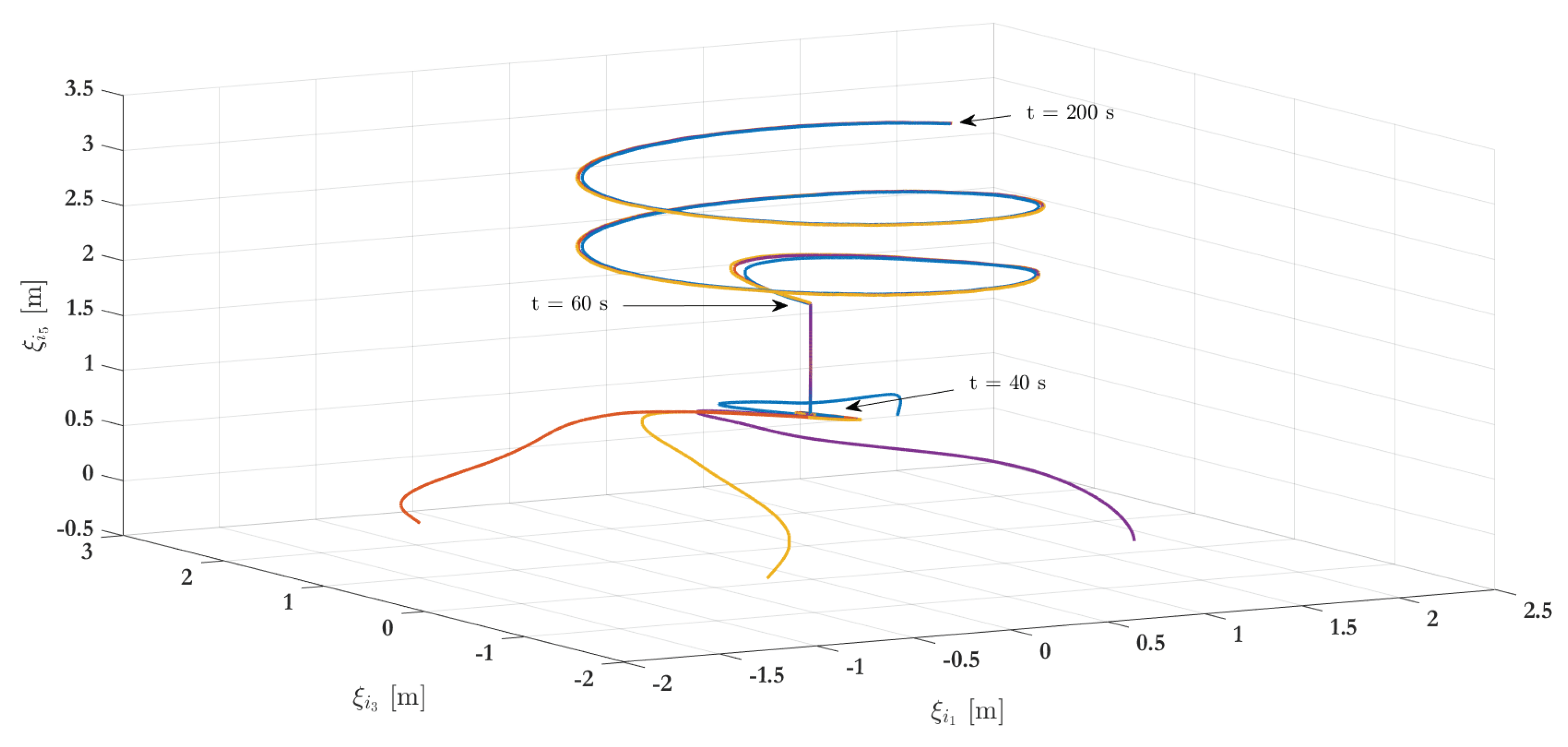
- The first scenario shows the consensus of four agents pursuing reference positions provided by the leader;
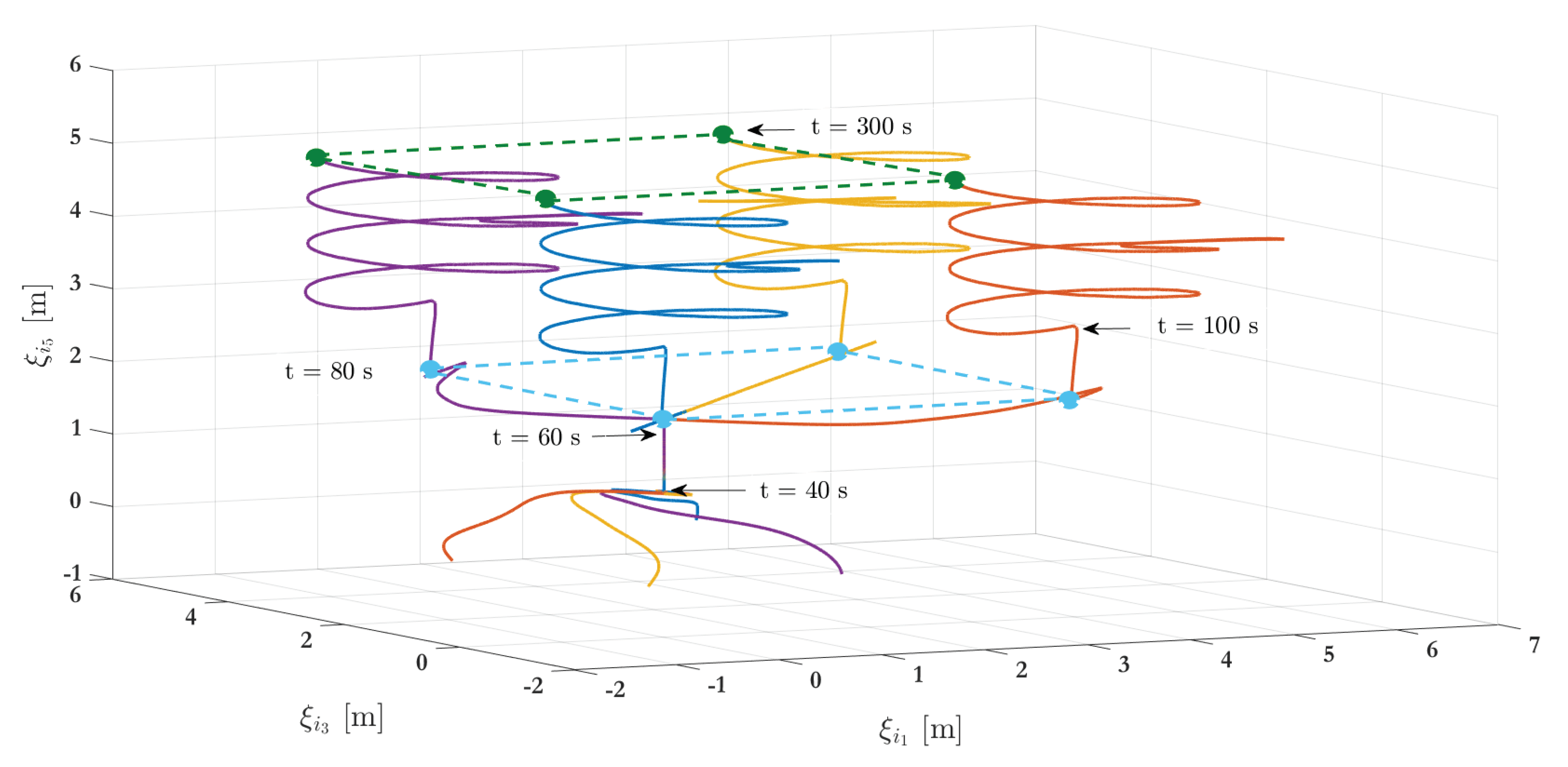
- A second one shows the evolution of the collaborative system for consensus and formation control. Moreover, the robustness to an external perturbation on one of the agents is illustrated.
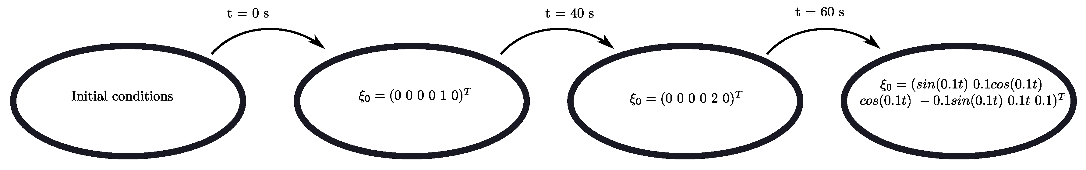
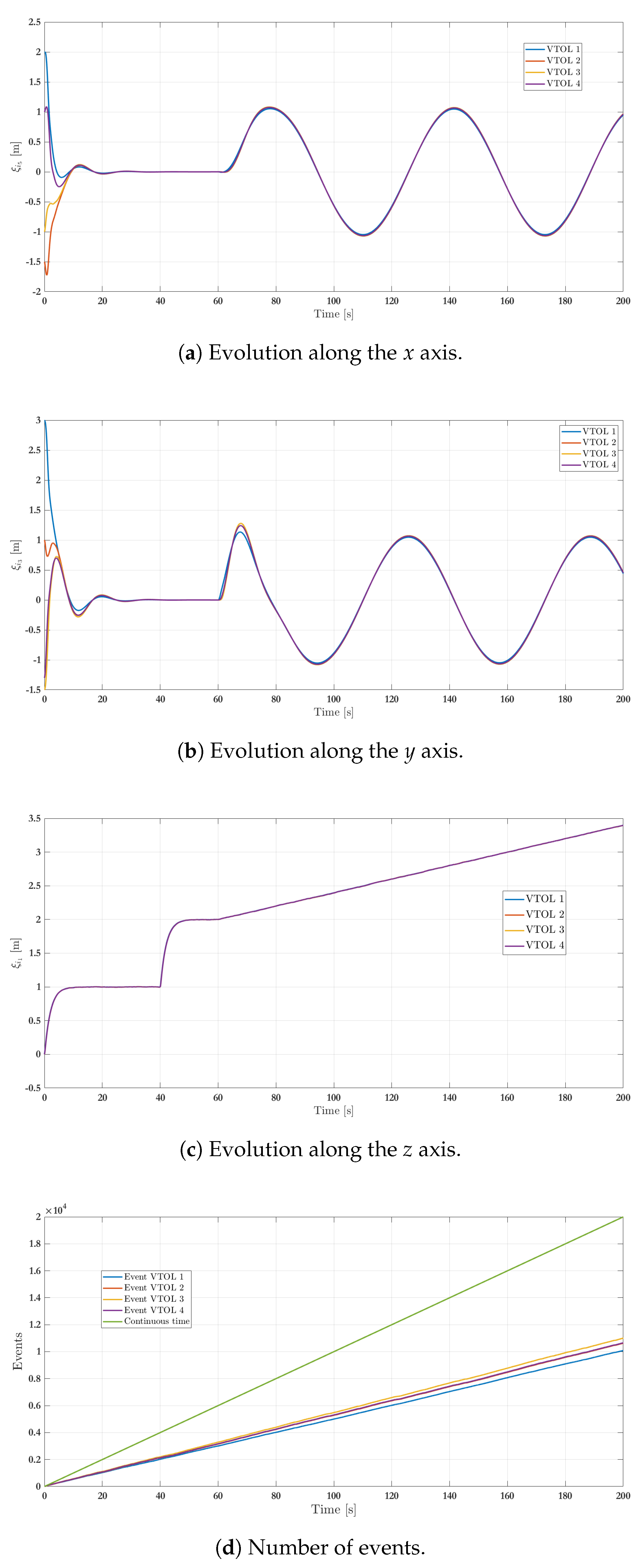
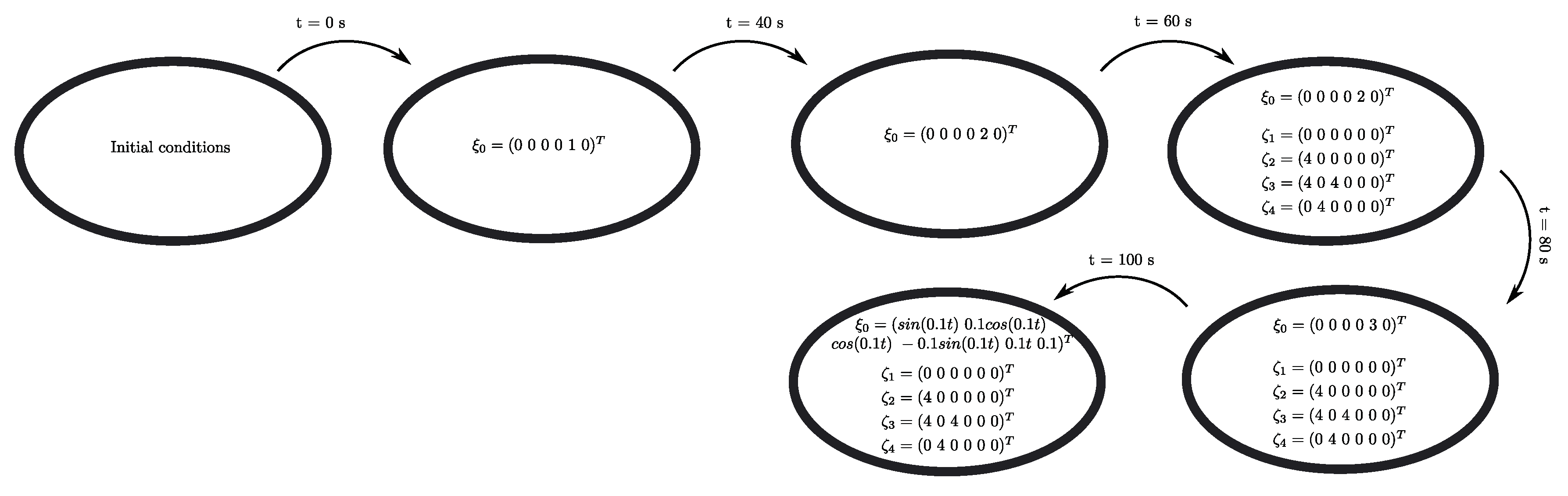
5.1.1. Scenario One
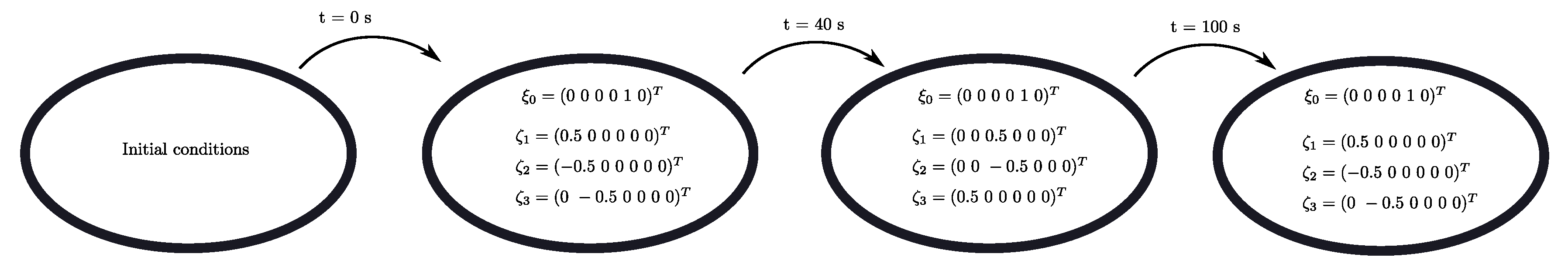
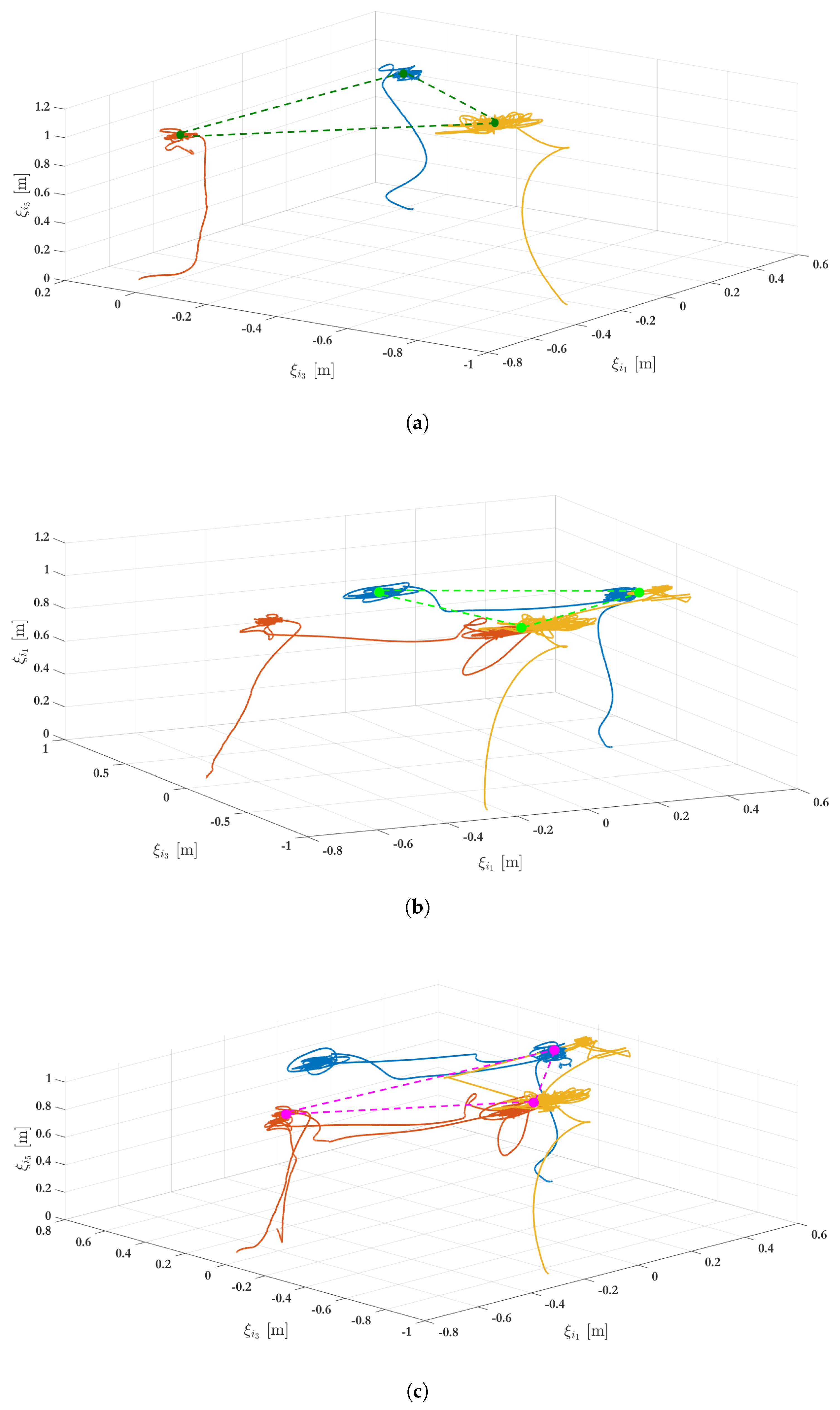
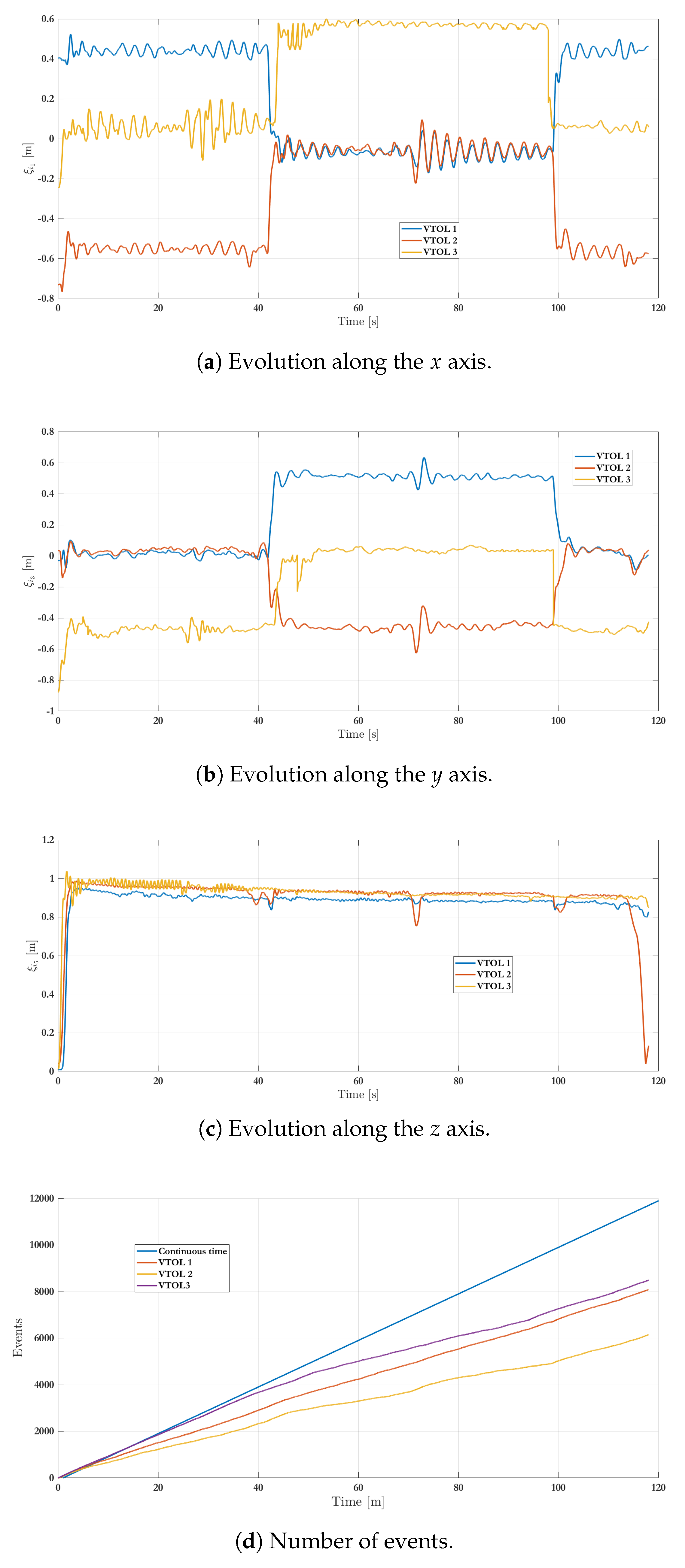
5.1.2. Scenario Two
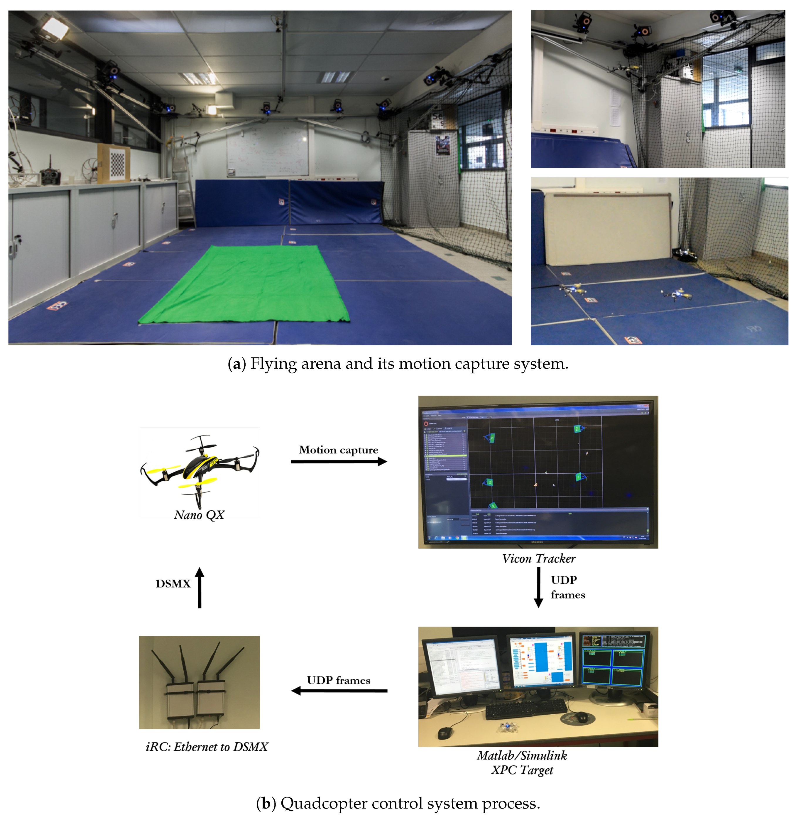
5.2. Experimental Results
6. Conclusions
Author Contributions
Funding
Acknowledgments
Conflicts of Interest
References
- Guerrero-Castellanos, J.F.; Vega-Alonzo, A.; Marchand, N.; Durand, S.; Linares-Flores, J.; Mino-Aguilar, G. Real-time event-based formation control of a group of VTOL-UAVs. In Proceedings of the 2017 3rd International Conference on Event-Based Control, Communication and Signal Processing (EBCCSP), Funchal, Portugal, 24–26 May 2017; pp. 1–8. [Google Scholar]
- Vega-Alonzo, A.; Guerrero-Castellanos, J.F.; Marchand, N.; Durand, S.; Mino-Aguilar, G.; Gonzalez-Díaz, V.R. Event-triggered leader-following consensus of UAVs carrying a suspended load. In Proceedings of the 2019 5th International Conference on Event-Based Control, Communication, and Signal Processing (EBCCSP), Vienna, Austria, 27–29 May 2019; pp. 1–8. [Google Scholar] [CrossRef]
- Song, H.; Rawat, D.B.; Jeschke, S.; Brecher, C. Front Matter. In Cyber-Physical Systems; Intelligent Data-Centric Systems, Academic Press: Boston, MA, USA, 2017; pp. i–ii. [Google Scholar]
- Martínez-Rey, M.; Espinosa, F.; Gardel, A.; Santos, C. On-Board Event-Based State Estimation for Trajectory Approaching and Tracking of a Vehicle. Sensors 2015, 15, 14569–14590. [Google Scholar] [CrossRef] [PubMed]
- Bradley, J.M.; Atkins, E.M. Optimization and Control of Cyber-Physical Vehicle Systems. Sensors 2015, 15, 23020–23049. [Google Scholar] [CrossRef] [PubMed]
- Ahmed, N.; Cortes, J.; Martinez, S. Distributed Control and Estimation of Robotic Vehicle Networks: Overview of the Special Issue. IEEE Control Syst. 2016, 36, 36–40. [Google Scholar]
- Ahmed, N.; Cortes, J.; Martinez, S. Distributed Control and Estimation of Robotic Vehicle Networks: Overview of the Special Issue-Part II. IEEE Control Syst. 2016, 36, 18–21. [Google Scholar]
- Thunberg, J.; Goncalves, J.; Hu, X. Consensus and formation control on SE(3) for switching topologies. Automatica 2016, 66, 109–121. [Google Scholar] [CrossRef]
- Peng, X.; Guo, K.; Geng, Z. Full State Tracking and Formation Control for Under-Actuated VTOL UAVs. IEEE Access 2019, 7, 3755–3766. [Google Scholar] [CrossRef]
- Du, H.; Zhu, W.; Wen, G.; Duan, Z.; Lü, J. Distributed Formation Control of Multiple Quadrotor Aircraft Based on Nonsmooth Consensus Algorithms. IEEE Trans. Cybern. 2019, 49, 342–353. [Google Scholar] [CrossRef]
- Olfati-Saber, R.; Murray, R.M. Consensus problems in networks of agents with switching topology and time-delays. IEEE Trans. Autom. Control 2004, 49, 1520–1533. [Google Scholar] [CrossRef]
- Bullo, F.; Cortés, J.; Martinez, S. Distributed Control of Robotic Networks: A Mathematical Approach to Motion Coordination Algorithms; Princeton University Press: Princeton, NJ, USA, 2009. [Google Scholar]
- Ren, W.; Beard, R.W. Distributed Consensus in Multi-Vehicle Cooperative Control; Springer: London, UK, 2008. [Google Scholar]
- Lewis, F.L.; Zhang, H.; Hengster-Movric, K.; Das, A. Cooperative Control of Multi-Agent Systems: Optimal and Adaptive Design Approaches; Springer Science & Business Media: London, UK, 2013. [Google Scholar]
- Monaco, S.; Normand-Cyrot, D. Advanced tools for nonlinear sampled-data systems’ analysis and control. In Proceedings of the 2007 European Control Conference (ECC), Kos, Greece, 2–5 July 2007; pp. 1155–1158. [Google Scholar]
- Miskowicz, M. Event-Based Control and Signal Processing; CRC Press: Boca Raton, FL, USA, 2015. [Google Scholar]
- Årzén, K.E. A Simple Event-Based PID Controller. In Proceedings of the 14th World Congress of IFAC, Beijing, China, 5–9 July1999. [Google Scholar]
- Åström, K.J.; Bernhardsson, B. Comparison of Riemann and Lebesque sampling for first order stochastic systems. In Proceedings of the 41st IEEE Conference on Decision and Control, Las Vegas, NV, USA, 10–13 December 2002; IEEE: Piscataway, NJ, USA, 2002; Volume 2, pp. 2011–2016. [Google Scholar]
- Tabuada, P. Event-triggered real-time scheduling of stabilizing control tasks. IEEE Trans. Autom. Control 2007, 52, 1680–1685. [Google Scholar] [CrossRef]
- Anta, A.; Tabuada, P. To sample or not to sample: Self-triggered control for nonlinear systems. IEEE Trans. Autom. Control 2010, 55, 2030–2042. [Google Scholar] [CrossRef]
- Mazo, M., Jr.; Anta, A.; Tabuada, P. On self-triggered control for linear systems: Guarantees and complexity. In Proceedings of the 2009 European Control Conference (ECC), Budapest, Hungary, 23–26 August 2009; IEEE: Piscataway, NJ, USA, 2009; pp. 3767–3772. [Google Scholar]
- Marchand, N.; Durand, S.; Guerrero-Castellanos, J.F. A general formula for event-based stabilization of nonlinear systems. IEEE Trans. Autom. Control 2013, 58, 1332–1337. [Google Scholar] [CrossRef]
- Dimarogonas, D.V.; Frazzoli, E.; Johansson, K.H. Distributed Event-Triggered Control for Multi-Agent Systems. IEEE Trans. Autom. Control 2012, 57, 1291–1297. [Google Scholar] [CrossRef]
- Seyboth, G.S.; Dimarogonas, D.V.; Johansson, K.H. Event-based broadcasting for multi-agent average consensus. Automatica 2013, 49, 245–252. [Google Scholar] [CrossRef]
- Garcia, E.; Cao, Y.; Casbeer, D.W. Decentralized event-triggered consensus with general linear dynamics. Automatica 2014, 50, 2633–2640. [Google Scholar] [CrossRef]
- Nowzari, C.; Cortes, J. Team-Triggered Coordination for Real-Time Control of Networked Cyber-Physical Systems. IEEE Trans. Autom. Control 2016, 61, 34–47. [Google Scholar] [CrossRef]
- Zimmerling, M.; Mottola, L.; Kumar, P.; Ferrari, F.; Thiele, L. Adaptive Real-Time Communication for Wireless Cyber-Physical Systems. ACM Trans. Cyber-Phys. Syst. 2017, 1, 8:1–8:29. [Google Scholar] [CrossRef]
- Muehlebach, M.; Trimpe, S. Distributed Event-Based State Estimation for Networked Systems: An LMI Approach. IEEE Trans. Autom. Control 2018, 63, 269–276. [Google Scholar] [CrossRef]
- Santos, C.; Espinosa, F.; Martinez-Rey, M.; Gualda, D.; Losada, C. Self-Triggered Formation Control of Nonholonomic Robots. Sensors 2019, 19, 2689. [Google Scholar] [CrossRef]
- Fan, Y.; Feng, G.; Wang, Y.; Song, C. Distributed event-triggered control of multi-agent systems with combinational measurements. Automatica 2013, 49, 671–675. [Google Scholar] [CrossRef]
- Zhu, W.; Jiang, Z.P.; Feng, G. Event-based consensus of multi-agent systems with general linear models. Automatica 2014, 50, 552–558. [Google Scholar] [CrossRef]
- Xing, L.; Wen, C.; Guo, F.; Liu, Z.; Su, H. Event-Based Consensus for Linear Multiagent Systems Without Continuous Communication. IEEE Trans. Cybern. 2017, 47, 2132–2142. [Google Scholar] [CrossRef] [PubMed]
- Cheng, Y.; Ugrinovskii, V. Event-triggered leader-following tracking control for multivariable multi-agent systems. Automatica 2016, 70, 204–210. [Google Scholar] [CrossRef]
- Xu, W.; Ho, D.W.C.; Li, L.; Cao, J. Event-Triggered Schemes on Leader-Following Consensus of General Linear Multiagent Systems Under Different Topologies. IEEE Trans. Cybern. 2017, 47, 212–223. [Google Scholar] [CrossRef] [PubMed]
- Yu, P.; Ding, L.; Liu, Z.W.; Guan, Z.H. Leader–follower flocking based on distributed event-triggered hybrid control. Int. J. Robust Nonlinear Control. 2016, 26, 143–153. [Google Scholar] [CrossRef]
- Li, W.; Liu, Y.; Sun, H. A survey of event-based consensus for multi-agent systems. In Proceedings of the 2017 Chinese Automation Congress (CAC), Jinan, China, 20–22 October 2017; pp. 6606–6611. [Google Scholar]
- Qin, J.; Ma, Q.; Shi, Y.; Wang, L. Recent Advances in Consensus of Multi-Agent Systems: A Brief Survey. IEEE Trans. Ind. Electron. 2017, 64, 4972–4983. [Google Scholar] [CrossRef]
- Ding, L.; Han, Q.; Ge, X.; Zhang, X. An Overview of Recent Advances in Event-Triggered Consensus of Multiagent Systems. IEEE Trans. Cybern. 2018, 48, 1110–1123. [Google Scholar] [CrossRef]
- Nowzari, C.; Garcia, E.; Cortes, J. Event-triggered communication and control of networked systems for multi-agent consensus. Automatica 2019, 105, 1–27. [Google Scholar] [CrossRef]
- Olfati-Saber, R.; Shamma, J.S. Consensus filters for sensor networks and distributed sensor fusion. In Proceedings of the 2005 44th IEEE Conference on Decision and Control and 2005 European Control Conference (CDC-ECC’05), Seville, Spain, 12–15 December 2005; IEEE: Piscataway, NJ, USA, 2005; pp. 6698–6703. [Google Scholar]
- Ni, W.; Cheng, D. Leader-following consensus of multi-agent systems under fixed and switching topologies. Syst. Control Lett. 2010, 59, 209–217. [Google Scholar] [CrossRef]
- Shuster, M.D. A survey of attitude representations. Navigation 1993, 8, 439–517. [Google Scholar]
- Schlanbusch, R.; Loria, A.; Nicklasson, P.J. On the stability and stabilization of quaternion equilibria of rigid bodies. Automatica 2012, 48, 3135–3141. [Google Scholar] [CrossRef]
- Guerrero-Castellanos, J.F.; Marchand, N.; Hably, A.; Lesecq, S.; Delamare, J. Bounded attitude control of rigid bodies: Real-time experimentation to a quadrotor mini-helicopter. Control Eng. Pract. 2011, 19, 790–797. [Google Scholar] [CrossRef]
- Sepulchre, R.; Jankovic, M.; Kokotović, P.V. Constructive Nonlinear Control; Springer: London, UK, 1997. [Google Scholar]
- Zavala, A.; Fantoni, I.; Lozano, R. Global stabilization of a PVTOL aircraft model with bounded inputs. Int. J. Control 2003, 76, 1833–1844. [Google Scholar] [CrossRef]


| Agent | Attitude | Position |
|---|---|---|
| VTOL 1 | (2, 8, −5) | (2, 3, 0) |
| VTOL 2 | (10, −15, 4) | (−1.5, 1, 0) |
| VTOL 3 | (−5, 10, −8) | (−1, −1.5, 0) |
| VTOL 4 | (−15, 7, −2) | (1, −1.3, 0) |
| Agent | Attitude | Position |
|---|---|---|
| VTOL 1 | ( −3.1, 3.4, 0.8) | ( 0.7, −0.6, 0) |
| VTOL 2 | ( 0.95, 0.99, 50.5) | ( 0.4, −0.03, 0) |
| VTOL 3 | ( −0.9, 0.53, 2.72) | ( −0.7, 0.03, 0) |
© 2019 by the authors. Licensee MDPI, Basel, Switzerland. This article is an open access article distributed under the terms and conditions of the Creative Commons Attribution (CC BY) license (http://creativecommons.org/licenses/by/4.0/).
Share and Cite
Guerrero-Castellanos, J.F.; Vega-Alonzo, A.; Durand, S.; Marchand, N.; Gonzalez-Diaz, V.R.; Castañeda-Camacho, J.; Guerrero-Sánchez, W.F. Leader-Following Consensus and Formation Control of VTOL-UAVs with Event-Triggered Communications . Sensors 2019, 19, 5498. https://doi.org/10.3390/s19245498
Guerrero-Castellanos JF, Vega-Alonzo A, Durand S, Marchand N, Gonzalez-Diaz VR, Castañeda-Camacho J, Guerrero-Sánchez WF. Leader-Following Consensus and Formation Control of VTOL-UAVs with Event-Triggered Communications . Sensors. 2019; 19(24):5498. https://doi.org/10.3390/s19245498
Chicago/Turabian StyleGuerrero-Castellanos, J. Fermi, Argel Vega-Alonzo, Sylvain Durand, Nicolas Marchand, Victor R. Gonzalez-Diaz, Josefina Castañeda-Camacho, and W. Fermin Guerrero-Sánchez. 2019. "Leader-Following Consensus and Formation Control of VTOL-UAVs with Event-Triggered Communications " Sensors 19, no. 24: 5498. https://doi.org/10.3390/s19245498
APA StyleGuerrero-Castellanos, J. F., Vega-Alonzo, A., Durand, S., Marchand, N., Gonzalez-Diaz, V. R., Castañeda-Camacho, J., & Guerrero-Sánchez, W. F. (2019). Leader-Following Consensus and Formation Control of VTOL-UAVs with Event-Triggered Communications . Sensors, 19(24), 5498. https://doi.org/10.3390/s19245498