1. Introduction
Hyperspectral sensors can collect abundant spectral information of target objects in hundreds of narrow bands. Hyperspectral images have extremely high spectral resolution, pixel-wise classification of which is the cornerstone of various hyperspectral applications, including agricultural yield estimation [
1], environment monitoring [
2], resource surveying [
3], and disaster monitoring [
4]. However, hyperspectral classification is still challenging due to high dimensionality, high nonlinearity, and the “small-sample problem” of hyperspectral data [
5,
6].
Research of hyperspectral classification is focused on the feature extraction and classifier designing [
7]. Classic feature extraction methods include principal components analysis (PCA) [
8], independent components analysis (ICA) [
9], linear discriminant analysis [
10], etc., aiming at dimensionality reduction and feature discrimination enhancement of hyperspectral data. Subspace clustering, which has a good theoretical foundation, is an important unsupervised representation learning method for high dimensional and large-scale data analysis [
11,
12]. Recently, subspace clustering has been successfully applied to hyperspectral classification in both an unsupervised manner and a supervised manner [
13,
14]. It is noteworthy that subspace clustering can be used as a powerful tool for band selection [
15,
16]. Classifiers designing combined with pattern recognition and machine learning is an effective solution for hyperspectral classification, and representative algorithms include support vector machine (SVM) [
17], multinomial logistic regression (MLR) [
18], extreme learning machines (ELMs) [
19], etc. Most earlier studies are based on spectral information, while spatial information has attracted more attention recently. Furthermore, a large number of literatures indicate that classification utilizing spatial–spectral information can effectively remove salt–pepper noise and generate better predicted maps [
20,
21,
22,
23]. High dimensionality, high nonlinearity, and limited training samples of hyperspectral data require feature extraction methods and classifiers to be capable of extracting and processing deep abstract features, making feature extraction the core issue of hyperspectral classification [
24]. However, most above-mentioned learning methods and classifiers, such as PCA, ICA, MLR, SVM, etc., are not based on a “deep” manner and deep architectures; on the contrary, can promote the re-use of features and learn more abstract features at higher layers of representations [
25]. For example, subspace clustering when employed as a deep model can better handle realistic data without the linear subspace structure [
26]. In recent years, deep learning has attracted much attention by providing an ideal solution for feature extraction. On the one hand, a deep learning model can extract features through active learning, with less human intervention and strong generalization ability [
27]. On the other hand, deep structures can extract hierarchical features with increasing levels of abstraction [
28]. Different from deep learning models, which take 1D vector as input, such as the stacked auto-encoder (SAE) [
29] and deep belief network (DBN) [
30], the convolutional neural network (CNN) [
31] can directly process 2D or 3D image data. Many important breakthroughs have been made in the field of computer vision by applying CNN, such as image classification [
31,
32,
33,
34], object detection [
35], and semantic segmentation [
36]. A large number of literatures have shown that CNN can effectively extract the deep spatial–spectral features directly from raw hyperspectral data blocks and achieve ideal classification accuracy [
37,
38,
39,
40,
41,
42].
A deep CNN model called AlexNet won the championship of the ImageNet Large Scale Visual Recognition Challenge (ILCVRS) in 2012, creating a giant wave of solving image processing issues with the study of the CNN model. Since then, VGG [
32], GoogleNet [
33], ResNet [
34], and other networks with excellent performance in the ILCVRS competition have overcome one milestone after another in CNN model research. In addition, the lightweight design of the CNN model has attracted more attention in recent years, aiming at reducing computational complexity. Xception [
43], SqueezeNet [
44], MobileNet [
45], ShuffleNet [
46], and other lightweight CNN models have been proposed successively. Researches on the CNN model strongly promote its penetration into related image processing areas. CNN-based hyperspectral classification mainly focus on hierarchical feature extraction with 2D-CNN or 3D-CNN. 2D-CNN-based hyperspectral classification mostly extract spatial features form hyperspectral data after dimension reduction [
37,
38]. The number of retained spectral bands and spatial window size vary from model to model. However, because of spectral information loss during 2D convolutional operation, the accuracy of 2D-CNN-based hyperspectral classification can be improved by utilizing 3D-CNN to extract spatial–spectral features. Chen et al. extract the deep spatial–spectral features from hyperspectral data using the 3D convolution kernel [
39]. The spatial window size is 27 × 27 and kernel size is 5 × 5 × 32. Li et al. built a 3D-CNN-based model with relatively small kernel and window size [
40]. Moreover, features with stronger discrimination can be extracted by optimizing the network structure of 3D-CNN. Hamida et al. alternatively used 3D convolution kernel of different scales to extract spatial–spectral features [
41]. He et al. used multi-scale convolution kernel in the same convolutional layer to extract spatial–spectral features, and then concatenated the extracted spatial–spectral features for hyperspectral classification [
42].
Hyperspectral data annotation is time-consuming and laborious, resulting in very limited labeled samples which can be used for training models. The “small-sample problem” has attracted more and more attention recently [
47,
48]. There are several mainstream methods in the machine learning field to solve the “small-sample problem” of hyperspectral classification, which are data augmentation [
39,
49], semi-supervised learning [
50,
51,
52], transfer learning [
53,
54], and network optimization [
55,
56,
57,
58]. Unlike the other three strategies, network optimization focuses on the model itself. Based on above observations, further optimizing the network structure to extract more discriminative features, and meanwhile improving the parameter using efficiency to avoid overfitting, is the focus of hyperspectral classification research based on 3D-CNN.
In terms of extracting discriminative features, theoretical research and image processing practice have proved that network depth is the key factor [
32,
33,
34,
59,
60]. By using residual connections in ResNet [
34], some researchers construct relatively deeper networks for hyperspectral classification. Lee et al. use 1 × 1 convolution kernels to learning hierarchical features extracted by the previous multi-scale convolution kernels, in which residual connections are used to make a network deeper [
55]. Liu et al. built a Res-3D-CNN of 12 layers with 3D convolution kernels and residual connections [
56]. Zhong et al. improved the position of residual connections and built a SSRN (Spectral–Spatial Residual Network) in which residual connections are used in the spectral feature learning and the spatial feature learning, respectively [
57]. In addition, structure innovation is also an important aspect of network optimization. Lately, Swalpa K R et al. proposed HybridSN, applying a 2D convolutional layer to further processing spatial–spectral features extracted by successive 3D convolutional layers [
58]. This concise and elegant model shows the giant potential of 2D-3D-CNN in hyperspectral classification by comparing it with previous state-of-the-art models, such as SSRN.
In order to better solve the “small-sample problem” of hyperspectral classification, we proposed a deeper 2D-3D-CNN called R-HybridSN (Residual-HybridSN). R-HybridSN not only inherits the advantages of some existing models, but also has considerably innovative designs. With a deep and efficient network structure, our proposed model can better learn deep hierarchical spatial–spectral features. Specially, the depth-separable convolutional layer proposed in Xception [
43] is used to replace the traditional 2D convolutional layer, aiming to reduce the number of parameters and further avoid overfitting.
2. Methodology
2.1. Proposed Model
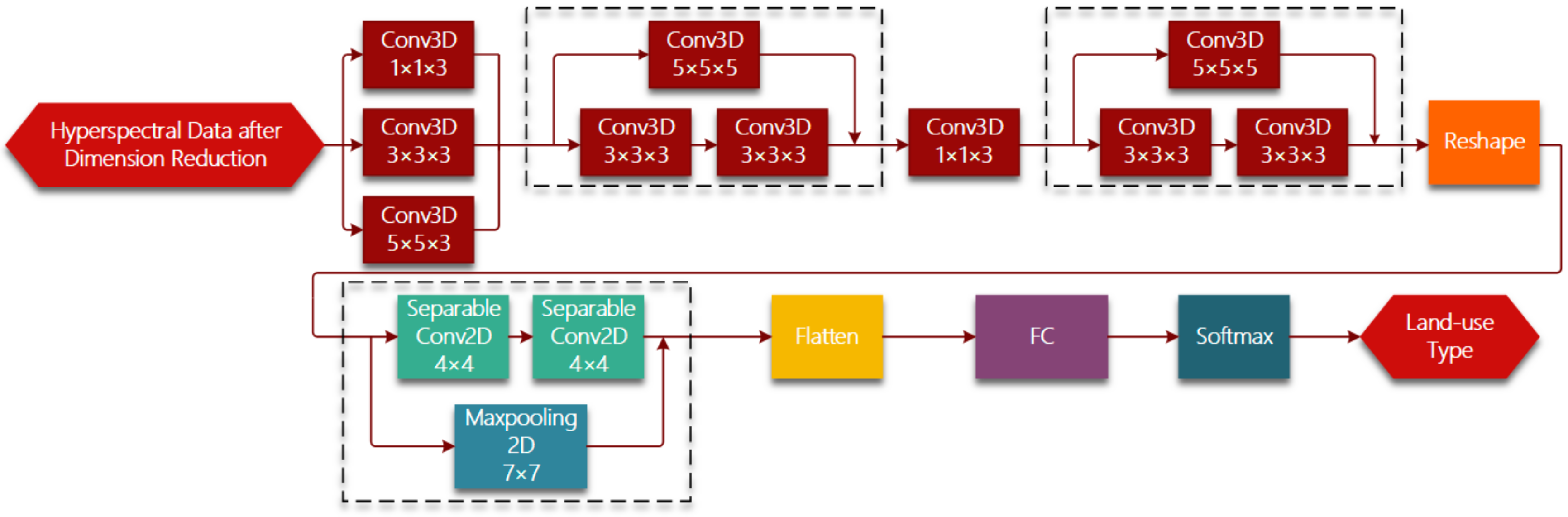
Figure 1 shows the whole framework of hyperspectral imagery classification based on R-HybridSN. In the light of lightweight designing, we conduct dimension reduction on raw hyperspectral data using PCA and keep a relatively small number of principle components. Hyperspectral data can be viewed as a 3D cube. Suppose the spatial size of hyperspectral data is
and the number of spectral bands is D, then the hyperspectral 3D cube can be denoted as
PCA is used in the spectral dimension of hyperspectral data. After selecting the first
principle components, the hyperspectral data can be denoted as
. The proposed R-HybridSN is based on 3D-CNN and accepts the 3D hyperspectral image patch as input, the land-use type of which is determined by the center pixel. A hyperspectral patch includes not only the spectral information of the pixel to be classified, but also the spatial information of the pixel within a certain range around. Every hyperspectral patch can be denoted as
, where
is the predefined neighborhood size.
The R-HybridSN has 11 layers and
Table 1 shows the output dimension of each layer, the number and size of convolution kernels. Reshape and Flatten module is applied for data dimension adjustment, the purpose of which is adapt to the data dimension requirement of next layer. Deep hierarchical spatial–spectral features are extracted by six successive 3D convolutional layers and two depth-separable 2D convolutional layers. In addition, we chose the widely used rectified linear unit (Relu) as the nonlinear activation function. After further abstract integration of spatial–spectral features, every pixel is classified with a specific land-use type in the output layer. Three residual connections are introduced to ease the training process of R-HybridSN and information from the upstream of the network is injected downstream. Specifically, the residual connections used in R-HybridSN include dimension adjustment. The position and dimension adjustment methods are shown in the dotted box in
Figure 1.
2.2. The 2D Convolution Operation
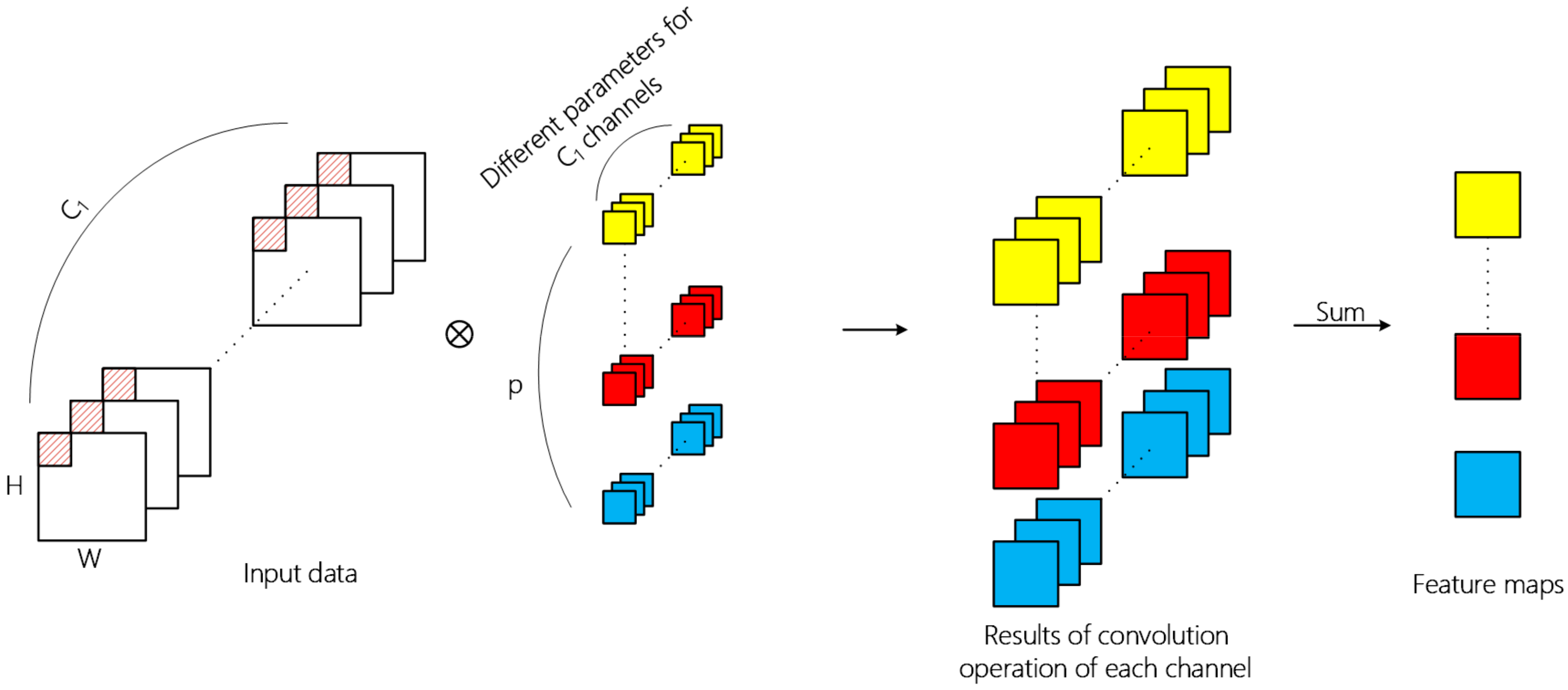
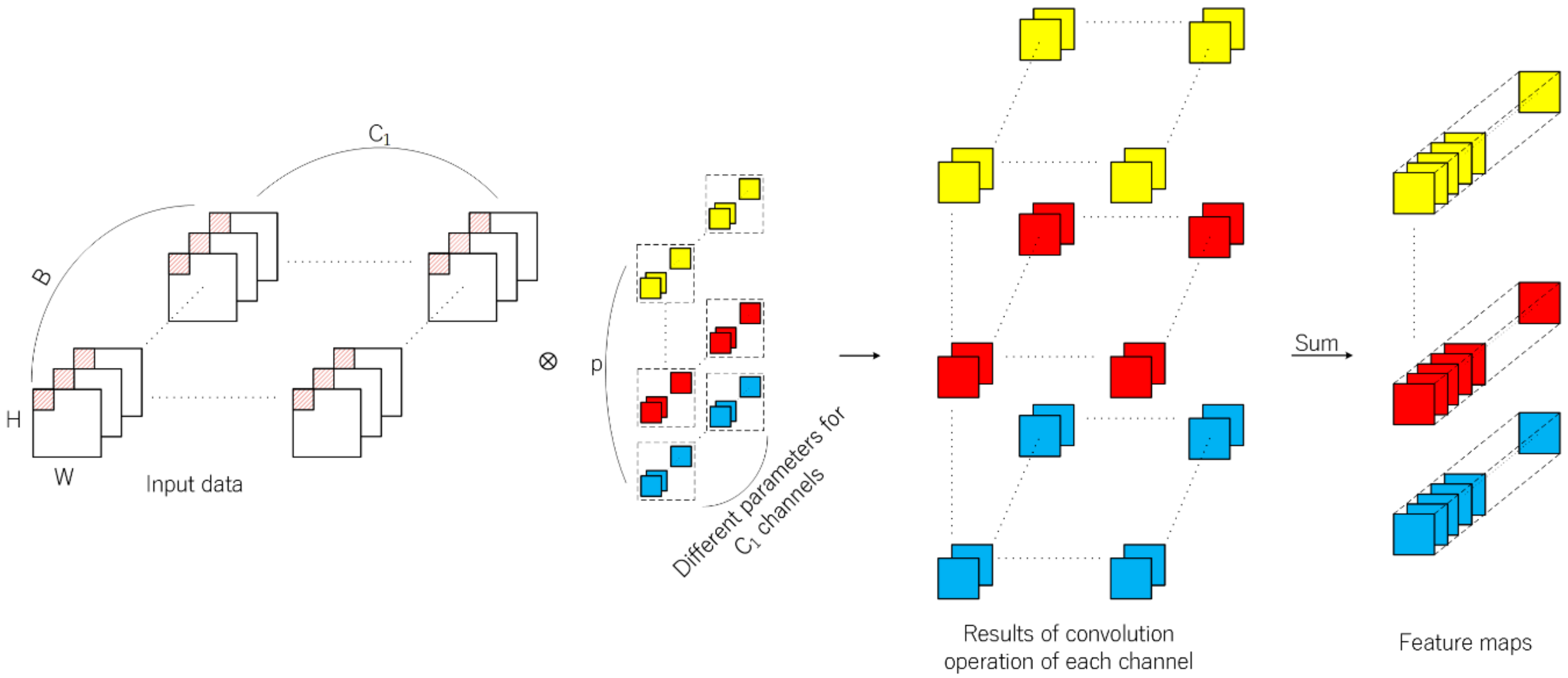
Convolutional neural networks are usually composed of input layer, convolutional layer, pooling layer, fully connected layer, and output layer. The convolutional layer is the core component for the extraction of deep hierarchical features. A convolutional layer extracts features by means of inner product of kernels in this layer and input data of the previous layer, in which convolutional kernel traverses all spatial positions of each channel of input data. The overall 2D convolution operation is shown in
Figure 2 and the value of the
position on the
th feature map at the
th layer is calculated by Formula (1),
where
represents the value at the position
of the
th convolution kernel in the
th layer, and the kernel convolutes the
th feature map of the previous layer;
and
represnets the size of the kernel;
represents the value at the position
of the
th feature map of the previous layer;
represents the output at the position
of the
th feature map in the
th layer;
represents the bias and
is the activation function. Different parameters are used for convolution operation in different channels, and the two-dimensional tensor obtained by summation of operation results is the feature extracted by the convolution kernel.
Through 2D convolution operation, one layer can learn local features from the previous layer and the kernel size determines local spatial size. Successive convolutional layer can increasingly abstract hierarchical features. In addition, the spatial feature learning and cross-channel feature learning in the ordinary 2D convolutional layer is carried out simultaneously. For the input 3D image data with length, width, and band, the operation result of multiple convolution kernels is also a 3D tensor. However, the depth dimension no longer corresponds to the band, but to the number of convolution kernels.
2.3. The 3D-CNN and 2D-3D-CNN
Different from 2D-CNN, feature learning is extended to the depth dimension by using 3D convolution kernels. The 3D convolution kernels conduct inner product across the spatial dimension and the depth dimension. Thus, it is suitable for the feature learning of hyperspectral data with rich spectral information. Firstly, R-HybridSN extracts spatial–spectral features using multi-scale 3D convolution kernels, in which padding is used to ensure the consistent dimension of input and output data. The operation results are concatenated in the spectral dimension as the output feature map of the first layer. The next step is to further integrate and abstract the spatial–spectral features with 5 successive convolutional layers. The process of 3D convolution operation is shown in
Figure 3. The calculation method of the position
of the
th feature cube in the
th convolutional layer is shown in Formula (2).
3D Convolution and 2D convolution have their own characteristics in feature extraction. In the 3D-CNN-based hyperspectral classification task, let the input data dimension, convolution kernel size, and the kernel number be respectively. In the 2D-CNN-based hyperspectral classification task, let the input data dimension, convolution kernel size, and the kernel number be , respectively. If padding is not used and the stride is 1, then the dimension of feature map is generated by 3D convolutional layer, and generated by 2D convolutional layer, respectively. In terms of network parameters, the number of weight parameters is for the 3D convolutional layer, and for the 2D convolutional layer. Therefore, on the one hand, the feature map generated by the 3D convolution operation contains more spectral information. On the other hand, the parameters of 3D convolutional layer are usually far more than those of 2D convolutional layer.
Inspired by HybridSN, the 2D convolutional layer is placed behind the successive 3D convolutional layers to further discriminates the spatial features. In order to fit the input dimension of 2D convolutional layer, the feature cubes generated by the 3D convolutional layer should be jointed in the spectral dimension, namely the dimension of the 4D tensor should be reshaped to . Different from HybridSN, R-HybridSN utilizes two depth-separable convolutional layers to enhance parameters using efficiency and residual connections to ease network training and to enhance the flow of spectral information in the network.
2.4. Depth-Separable Convolution
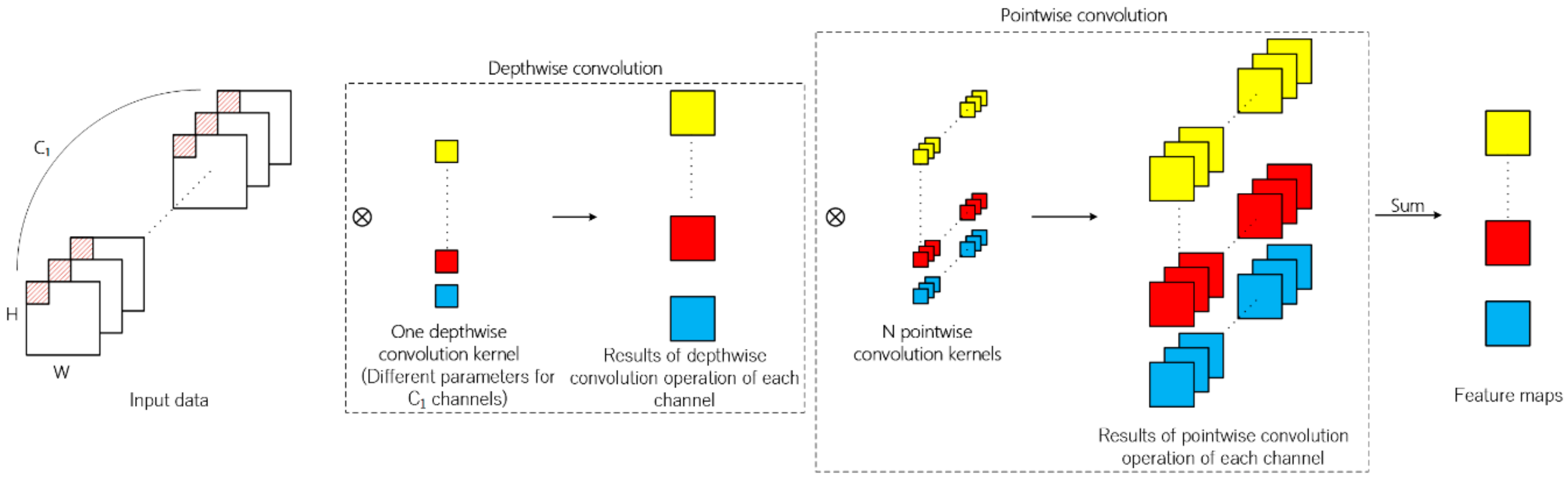
It can be observed from the operation process of traditional 2D convolution that in terms of feature map generation, the information of spatial dimension and channel dimension is mapped simultaneously. Different from traditional 2D convolution, depth-separable convolution can be divided into depthwise convolution and pointwise convolution. Firstly, every channel of input data is convoluted by 2D convolution kernels and the number of kernels is usually set to one in depthwise convolution. The second step is similar to traditional 2D convolution of which kernel size is 1 × 1. The above operation process is illustrated in
Figure 4.
Compared with the traditional 2D convolution, depth-separable convolution both reduces the number of parameters and the calculation times in the network, thus speeding up the network training and reducing the possibility of overfitting in the classification task. Suppose that the channel number of input feature map is , the size of convolution kernel is , the number of depthwise convolution kernel is q, the number of pointwise convolution kernel is N, and the size of the generated feature map is . The number of parameters in the traditional convolutional layer is and the number of parameters in the depth-separable convolutional layer is . The times of multiplications is for the traditional convolutional layer and for the depth-separable convolutional layer, respectively. The ratios on parameters and times of multiplications of traditional convolutional layer to depth-separable convolutional layer are both . Since q is usually set to 1, using depth-separable convolution can greatly reduce the number of parameters and the calculation times required.
The performance of hyperspectral classification can be improved by applying depth-separable convolution. First, the number of parameters and calculation times are reduced. Second, the concatenated feature map generated by successive 3D convolutional layers can be considered to contain extremely abundant spectral information in a certain neighborhood of the pixel to be classified. The depth-separable convolution is very suitable for the data structure of the concatenated feature map, of which the size depth dimension is far larger than that of spatial dimension.
2.5. Residual Learning
The theoretical research on the feedforward deep network indicates that the depth of the network has an exponential advantage over the width of the network (namely the number of neurons in the same layer) in terms of function fitting ability [
59,
60]. In addition, the image classification practice based on CNN shows that the deep network can learn abstract features better [
32,
33,
34]. Therefore, deep network construction is an important strategy to deal with the challenge of hyperspectral classification. And in terms of constructing deep network for “small-sample problem”, the key point is reducing training difficulty and avoid overfitting.
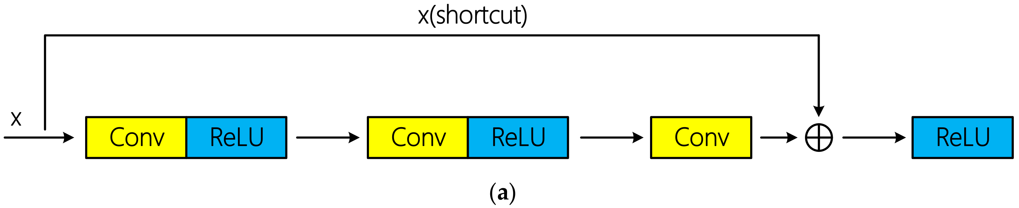
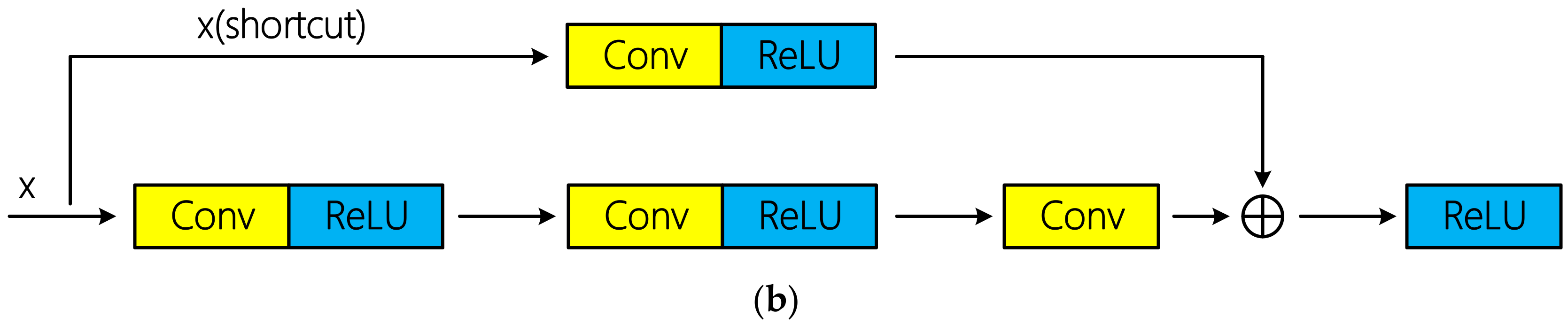
The training of the deep convolutional neural network can be successfully realized through residual connection proposed in literature [
34]. Residual connections can be divided into identity connection and non-identity connection according to whether there is dimension adjustment. Schematic diagram of the two types of residual connections is shown in
Figure 5. Tensor addition requires same dimension. If the input x does not change its dimension after several convolutional layers, x can be directly injected into the downstream of the network by using identity connection; otherwise, dimension adjustment is required. Specially, [
34] indicated that identity connection is sufficient to solve the degradation problem of deep network, and is more economical and practical than non-identity connection with dimension adjustment. In the mentioned hyperspectral classification researches above based on residual learning, all the authors used identical connection and achieved excellent classification performance.
However, there are three non-identity residual connections in R-HybridSN. The first two residual connections occurred among the successive 3D convolutional layers, and the 3D convolutional layer was used to conduct the dimension adjustment. In addition, the dimension adjustment in the third residual connection is done by a max pooling layer. The reasons why identical residuals are not used in this article are as follows:
From the perspective of network structure, identical connection requires consistent input and output dimensions, which reduces the flexibility of model construction to some extent. Thus, we aim to explore the classification performance of hyperspectral data using non-identity residual connection.
Residual connections with convolutional layers make the network more like directed acyclic graphs of layers [
61], in which each branch has the ability to independently extract spectral-spectral features.
The feature map generated by the Reshape module is believed to contain extremely rich spectral information. However, due to the mode of feature map generating used by subsequent 2D convolutional layers, the extracted spectral features suffer some losses. In order to better realize spatial–spectral association, we add the feature map generated by the Reshape module to the feature map generated by the last 2D convolutional layer, enhancing the flow of spectral information in the R-HybridSN.
3. Datasets and Contrast Models
To verify the performance of the proposed model, we use three public available hyperspectral datasets, namely Indian Pines, Salinas, and University of Pavia. The Indian Pines, Salinas, and University of Pavia datasets are available online at
http://www.ehu.eus/ccwintco/index.php?title=Hyperspectral_Remote_Sensing_Scenes. We use some public available codes to prepare the training and testing data, compute the experimental results and implement the M3D-DCNN as one of the contrast models. The codes are available online at
https://github.com/gokriznastic/HybridSN and
https://github.com/eecn/Hyperspectral-Classification. Indian Pines consists of 145 × 145 pixels with a spatial resolution of 20 m. The bands covering the water absorption region were removed and the remaining 200 bands are used for classification. The Indian Pines scene mainly contains different types of crops, forests, and other perennials. The ground truth available is designed to sixteen classes. Salinas consists of 512 × 217 pixels with a spatial resolution of 3.7 m. As with Indian Pines, the water absorption bands were discarded and the number of remaining bands is 204. The Salinas scene mainly consists of vegetation, bare soil, and vineyards. The labeled samples are divided into 16 classes, total of which is 54,129. The University of Pavia consists of 610 × 340 pixels with a spatial resolution of 1.3 m. The labeled samples are divided into 9 classes, most of which are the features of the town, such as metal plate, roof, asphalt pavement, etc. The total number of labeled samples is 42,776.
Most of CNN-based hyperspectral classification algorithms are supervised and the number of training samples are of great significance to the classification accuracy. The same three datasets were used in [
58] and the proportion of training samples used was 30%. In addition, supplementary experiments using 10% labeled data as training samples were conducted to further observe the performance of HybridSN. In [
57], 20% labeled data were used to train SSRN for Indian Pines, and 10% for University of Pavia, respectively.
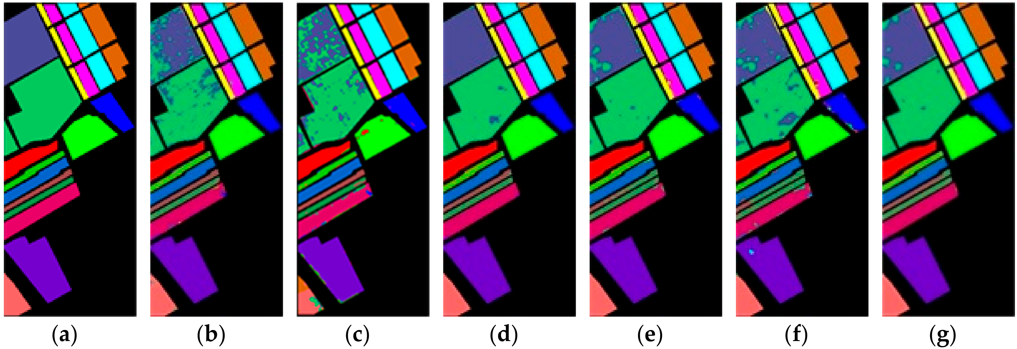
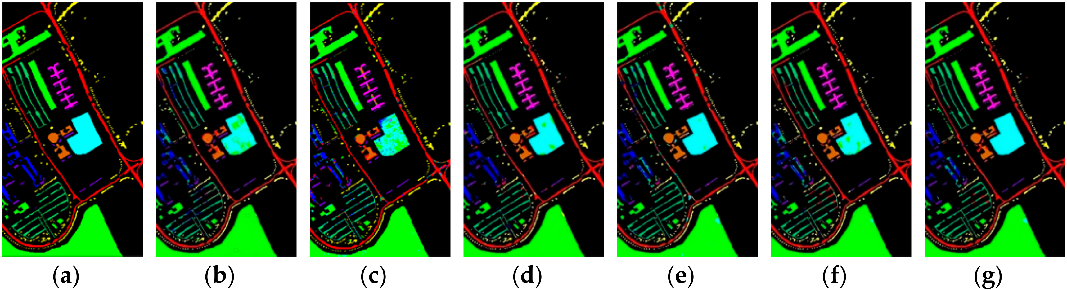
In our experiment, the number of training samples was further reduced to observe the classification performance of R-HybridSN. In addition, different from the common setting of most hyperspectral classification experiments, we do not use the same amount of training samples for each class in this paper. Instead, the training sample ratio of each ground object class is consistent with that in the total labeled samples. Three landmark CNN-based hyperspectral classification models—2D-CNN [
37], M3D-DCNN [
42], and HybridSN [
58]—are compared with our proposed R-HybridSN. In addition, in order to observe the impact of residual learning and depth-separable convolution in R-HybridSN on classification performance, we built the following two extra contrast models, namely Model A and Model B. Model A replaces the part of depth-separable convolution with traditional 2D convolution and Model B removes residual connections from R-HybridSN. The other settings are consistent with R-HybridSN.


