Design and Implementation of a Novel Tilt Sensor Based on the Principle of Variable Reluctance


Abstract
:1. Introduction
- (1)
- It is the first time the novel structure of a sensor with a measurement range of 360° is presented. According to the requirement, sensors with this structure can be made very large or very small.
- (2)
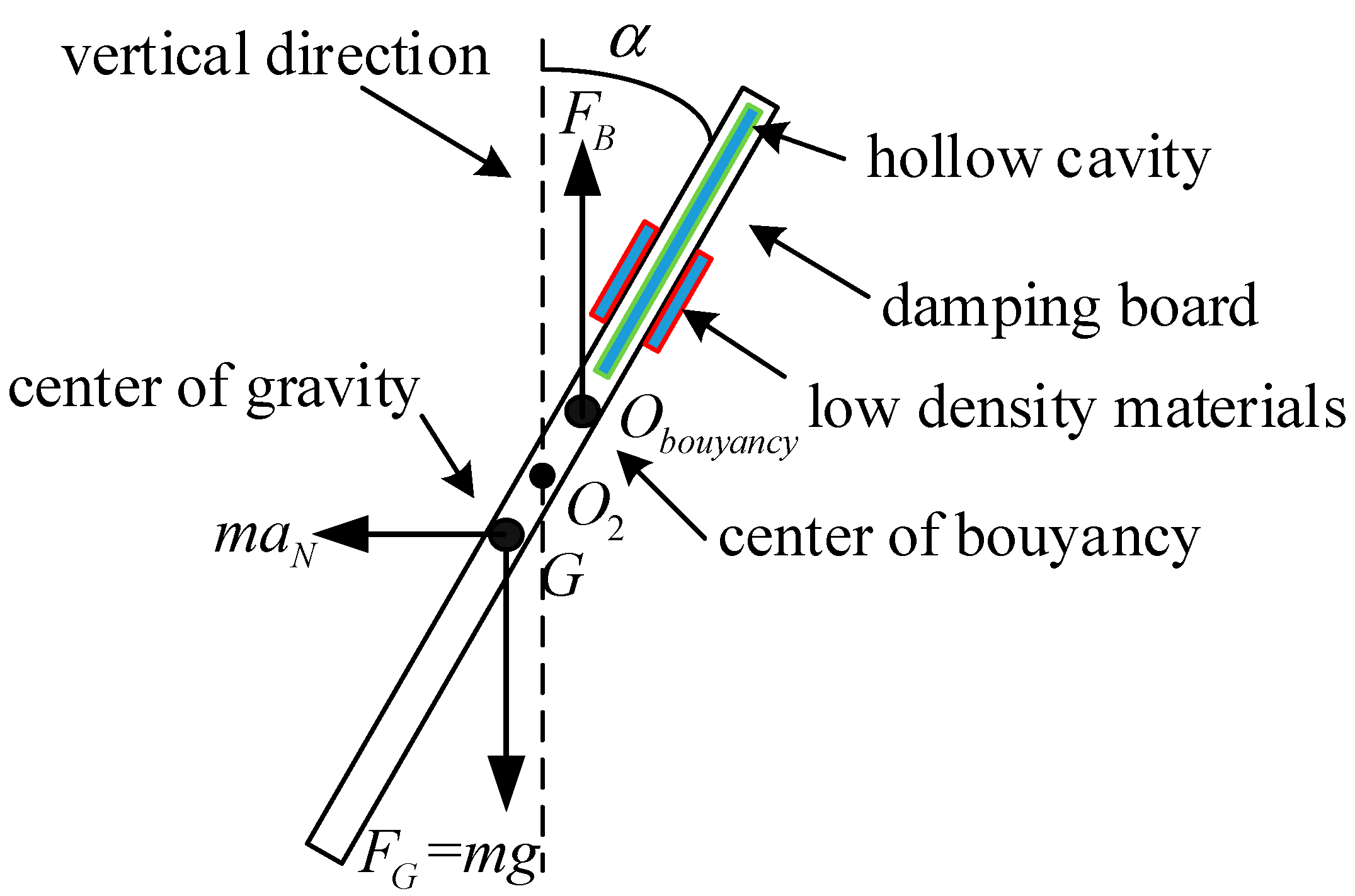
- In order to reduce the influence of translation noise, the sensor is filled with oil. A damping board fixed in the sensor, with the structure of a buoyancy center moving up from the geometric center and the gravity center moving down from the geometric center is proposed.
- (3)
- A scheme of non-electricity conversion is proposed. Mechanical motion such as roll angle is transformed into the variation of reluctance. The variation of reluctance causes the change of inductance value of the sensor coil. The change of inductance leads to the change of output frequency of the clapper oscillator circuit.
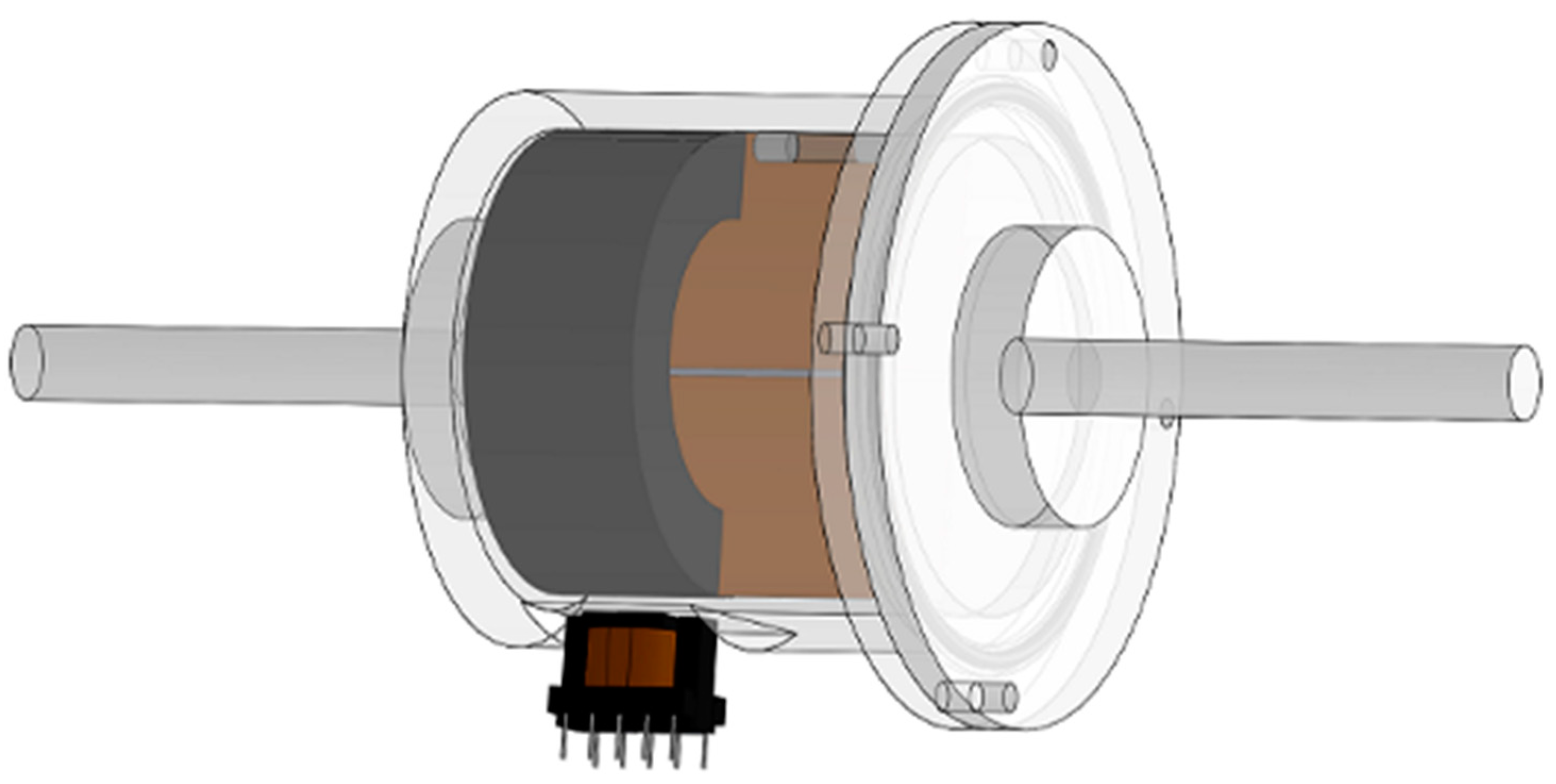
2. Sensor Structure Design
3. Theoretical Analysis
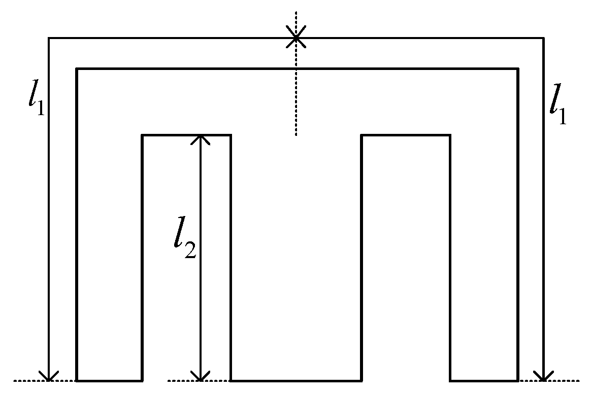
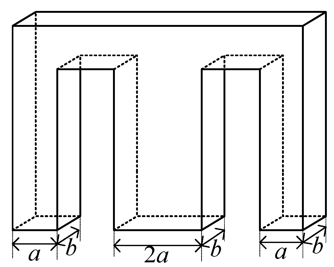
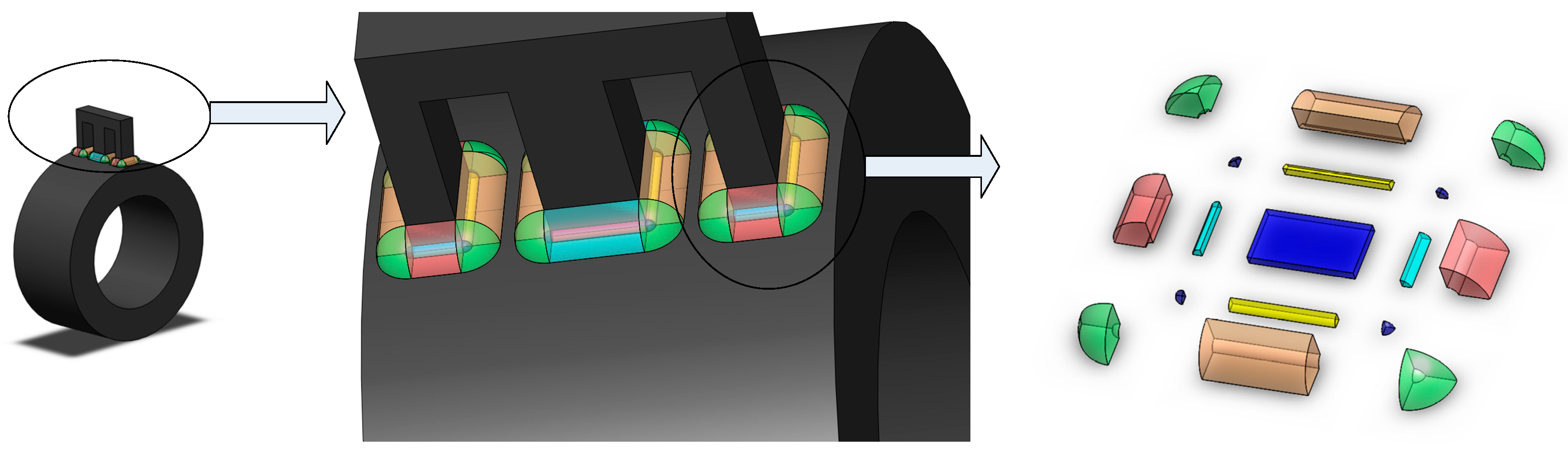
3.1. Sensor Analysis of Gas Gap in the Sensor
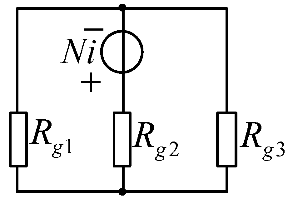
3.2. Reluctance Analysis of the Sensor
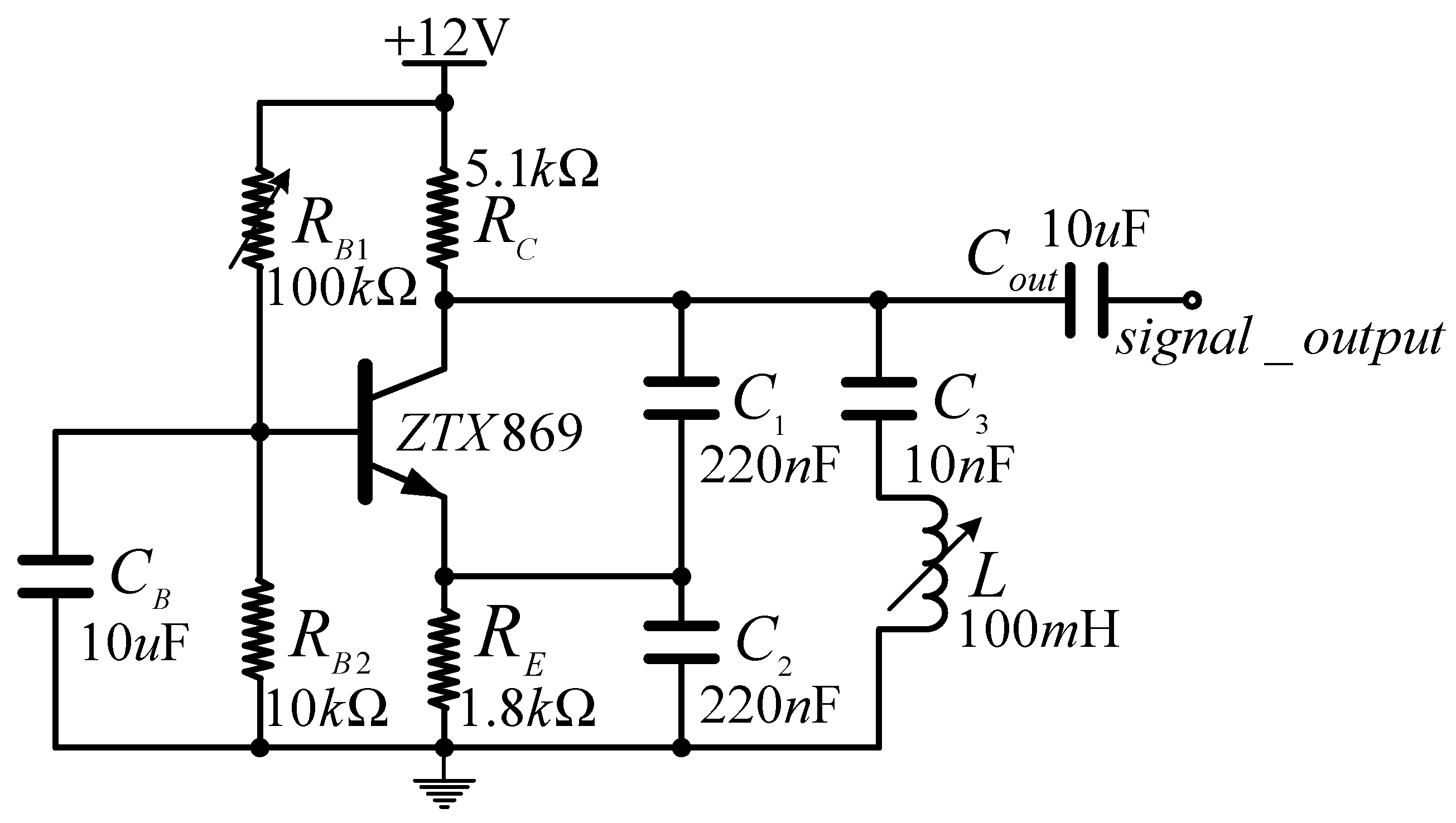
3.3. Design of the Clapp Oscillator
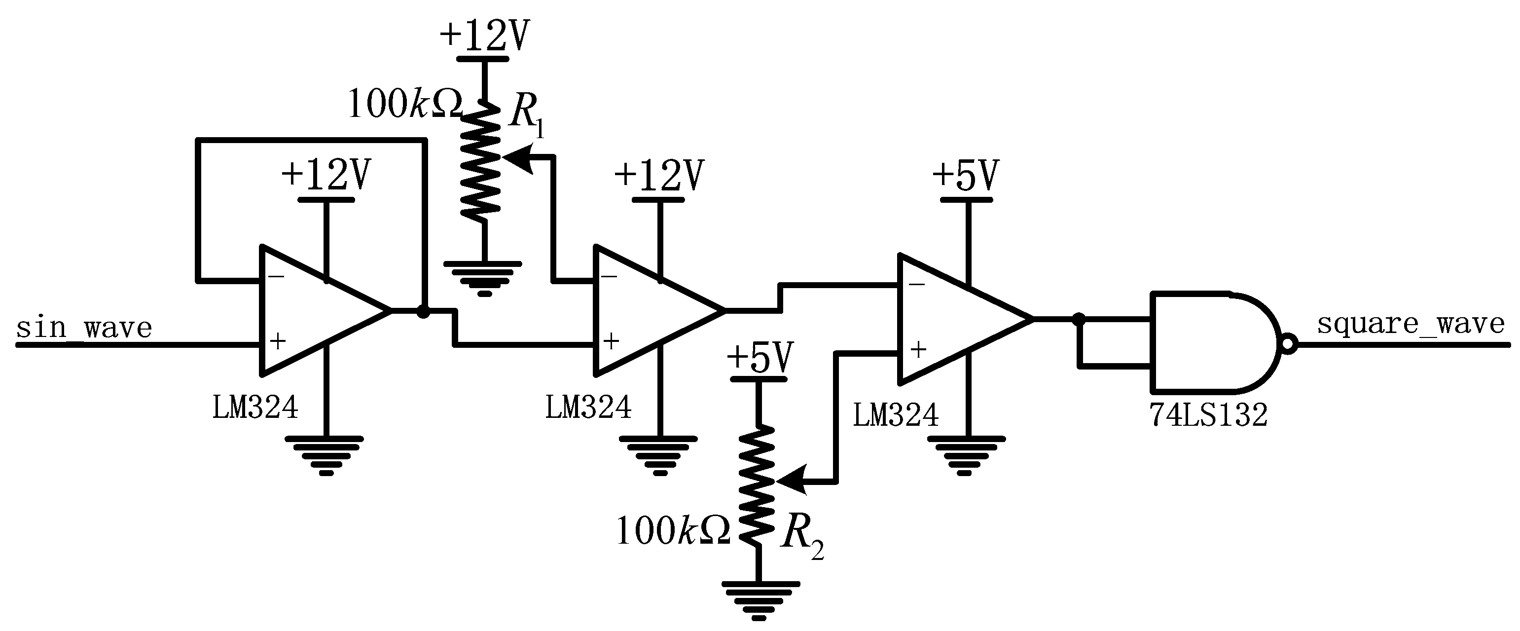
3.4. Design of the Waveform Conversion Circuit
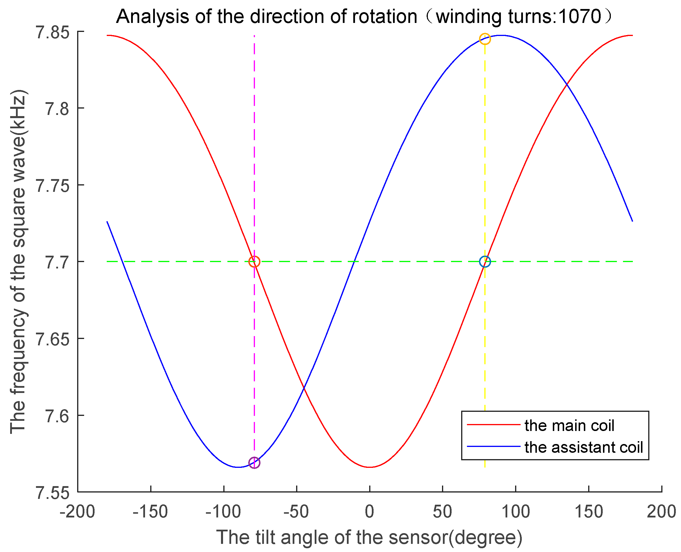
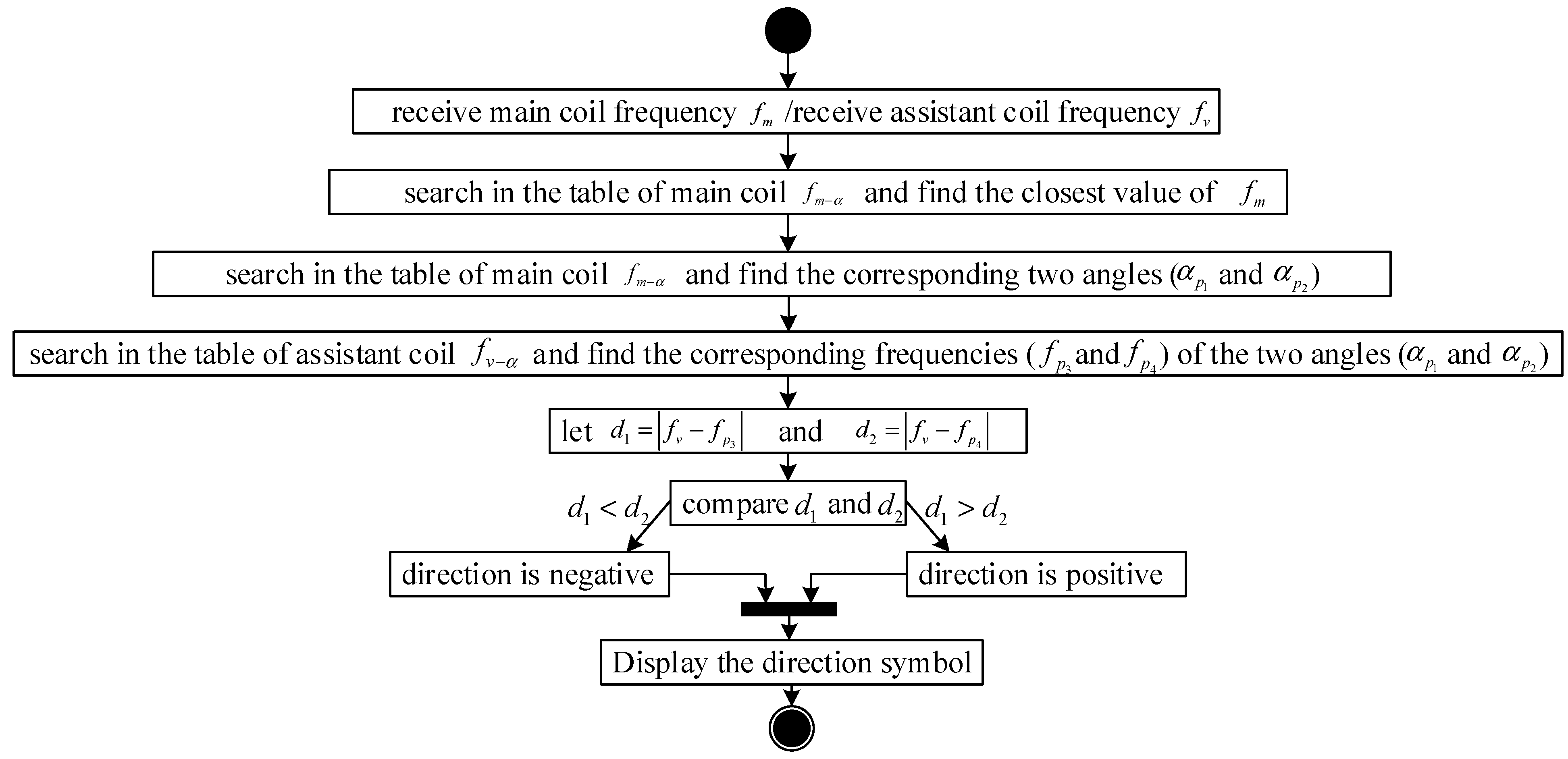
3.5. Analysis of the Sensor’s Direction of Rotation
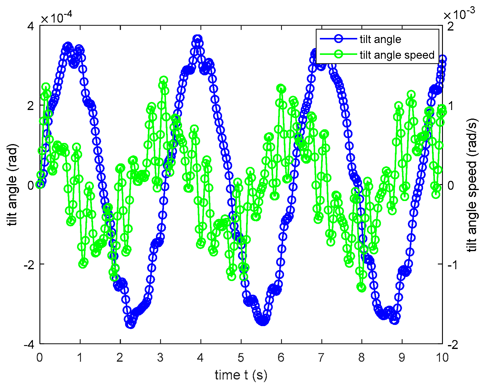
3.6. Theoretical Analysis of the Sensor’s Dynamic Characteristics
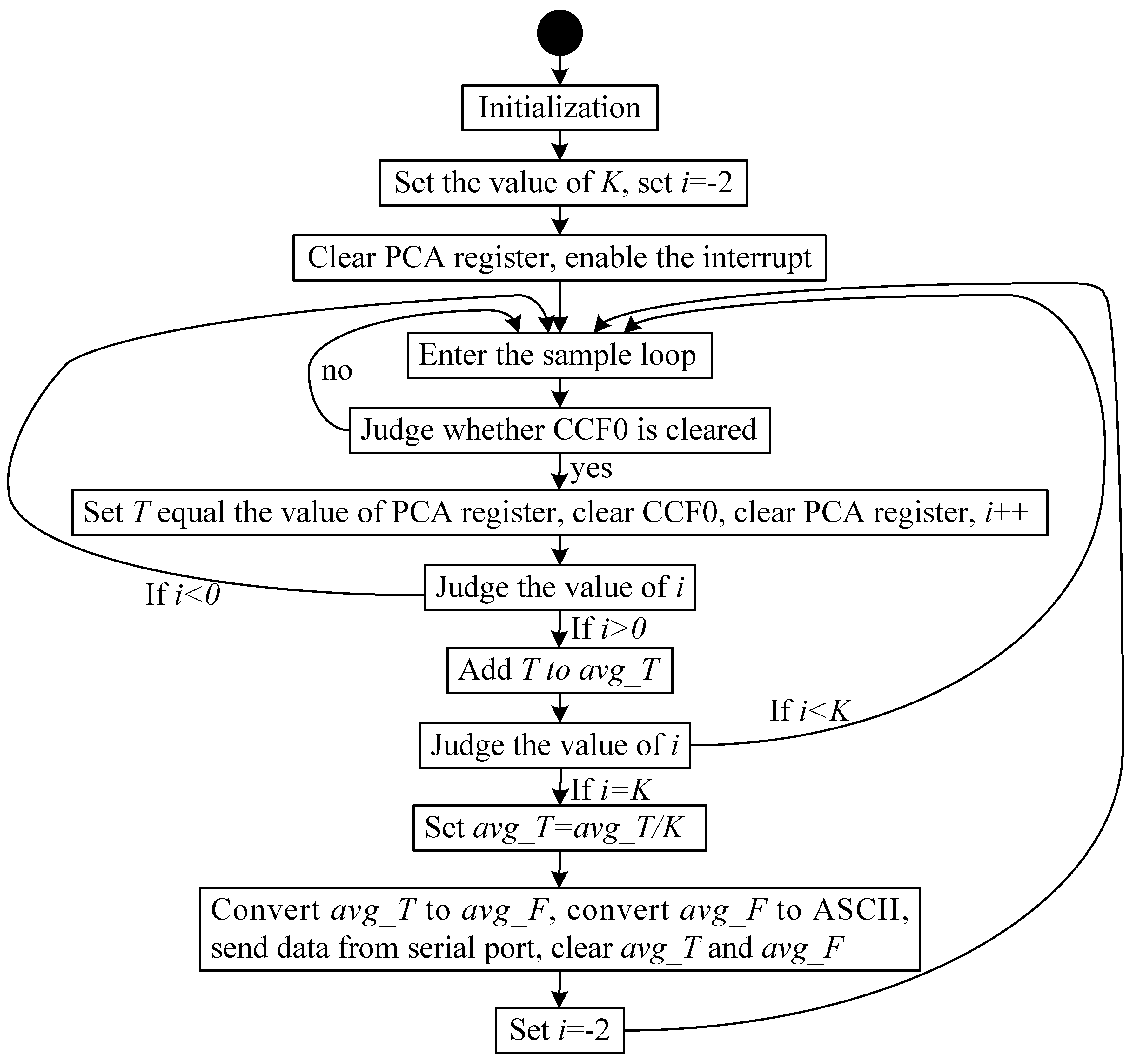
3.7. Design of the Frequency Meter
4. Experimental Section
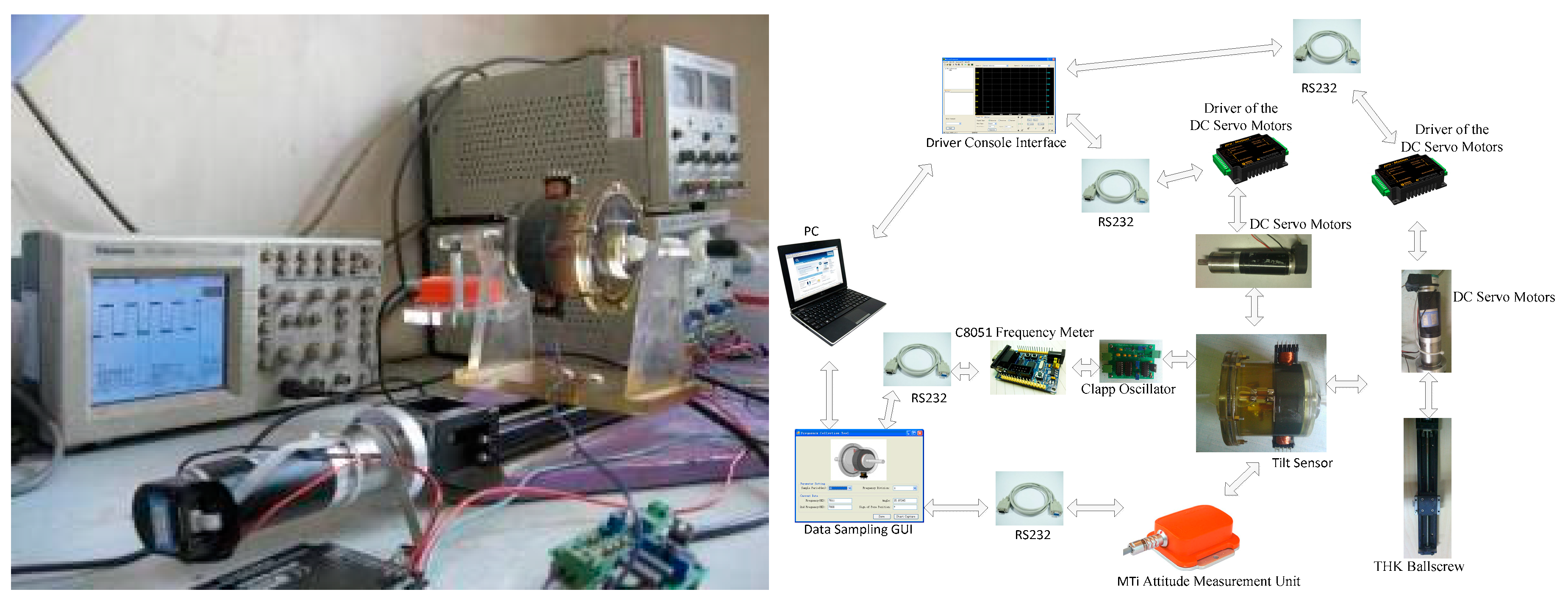
4.1. Design of the Experimental Hardware Platform
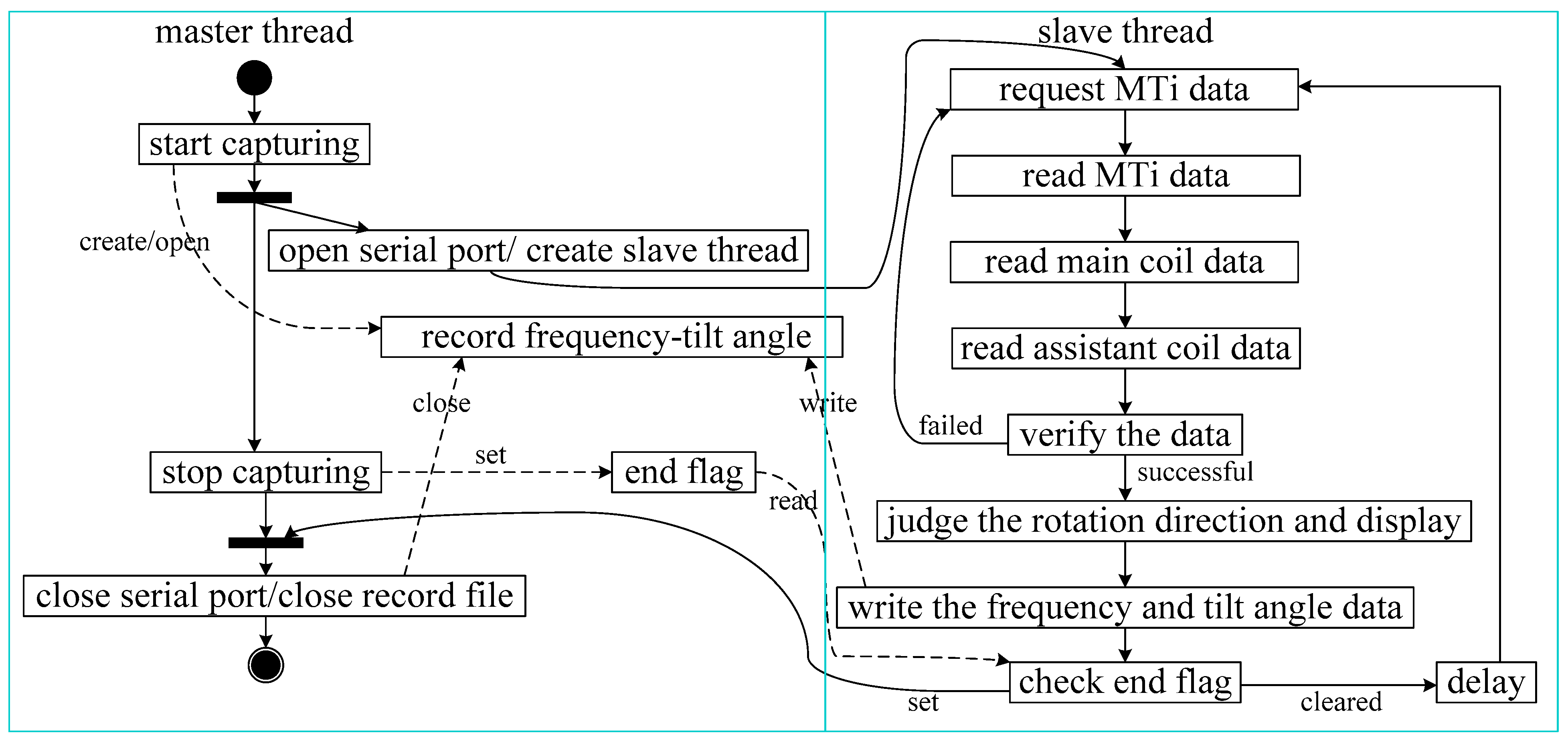
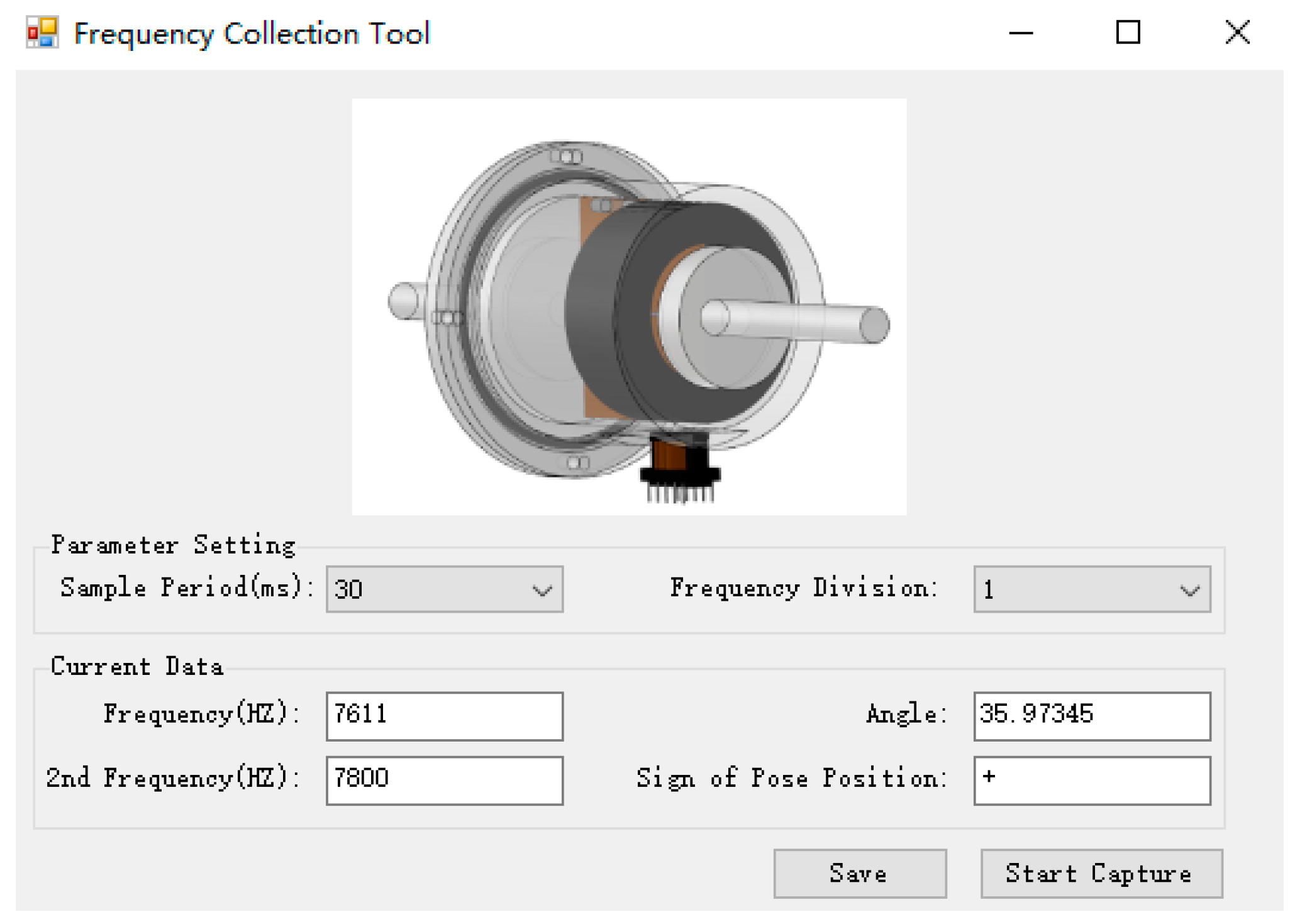
4.2. Design of Experimental Software Platform
5. Results and Discussion
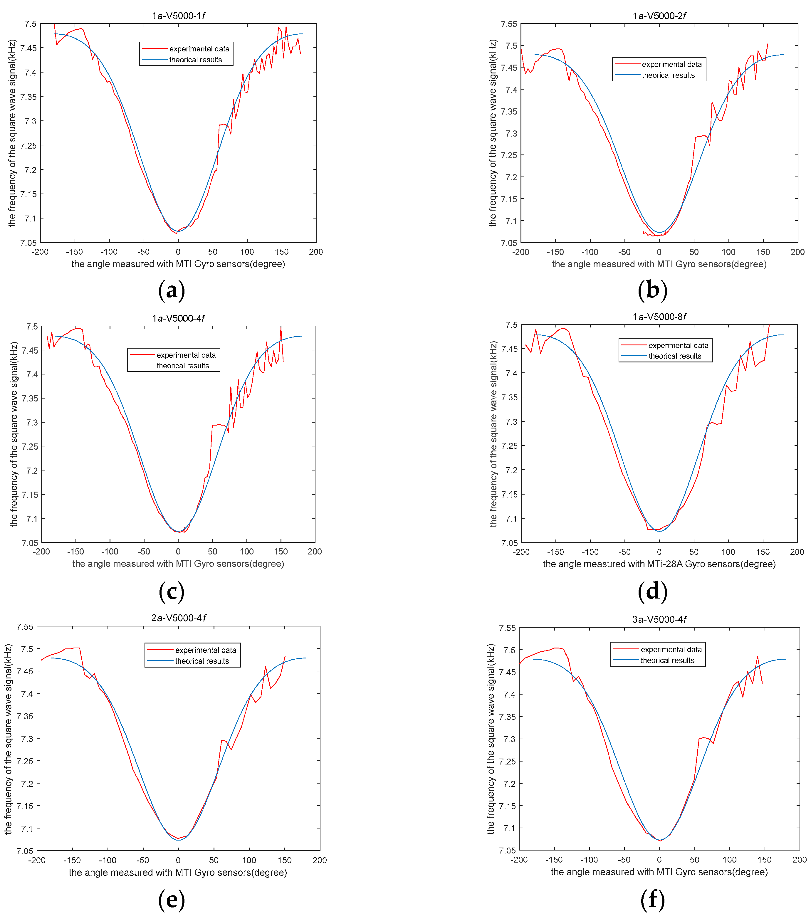
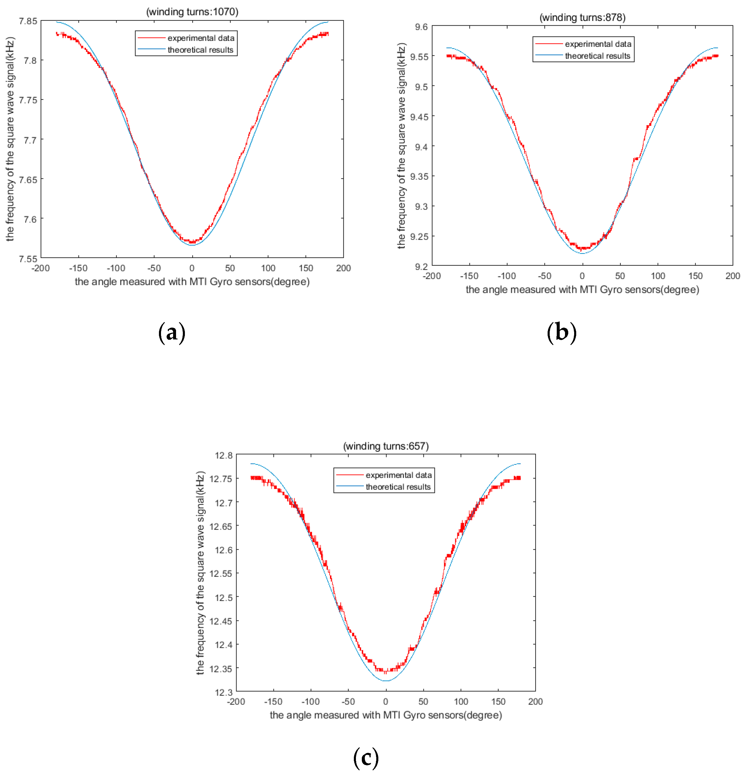
5.1. Experiments of the Sensor in Pure Rotation
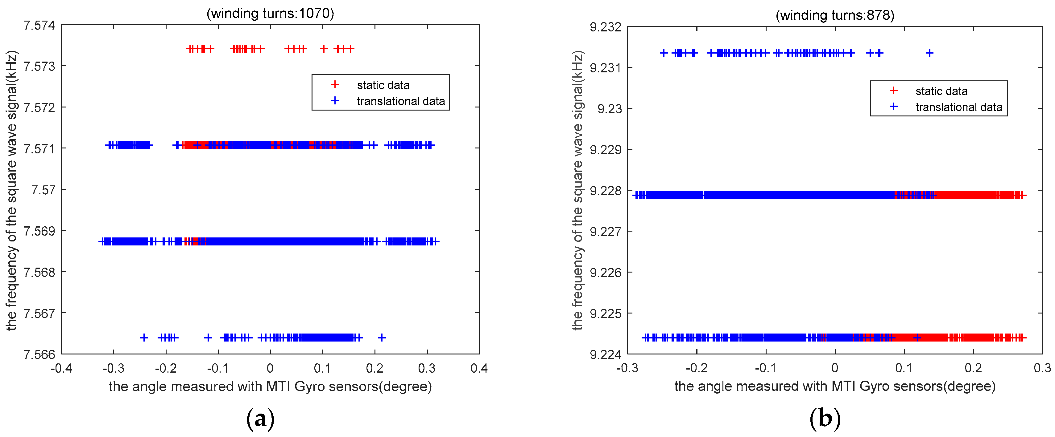
5.2. Experiments of the Sensor in Rotation with Translational Interference
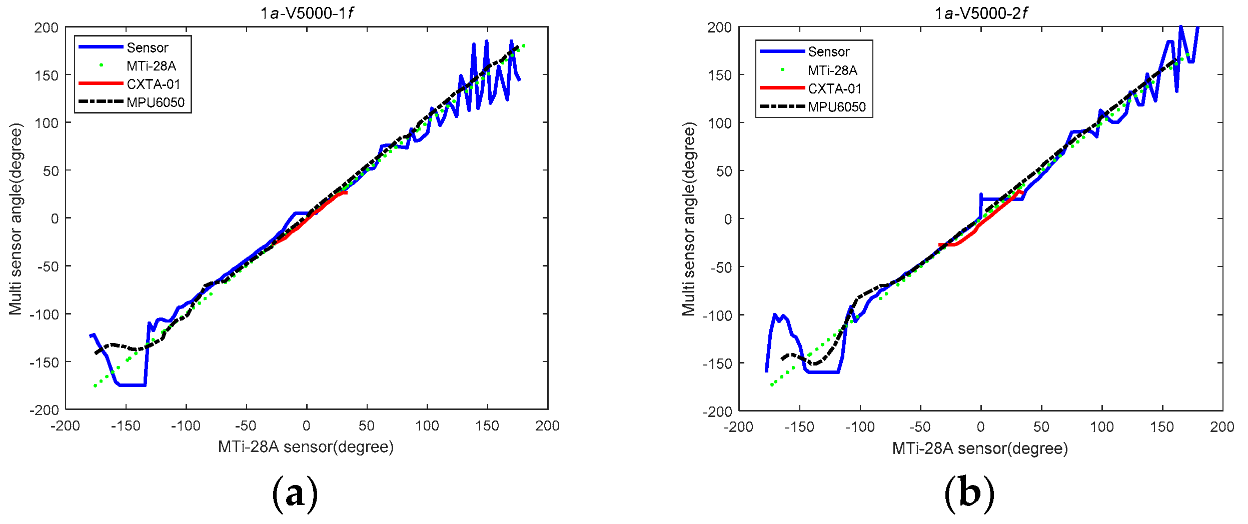
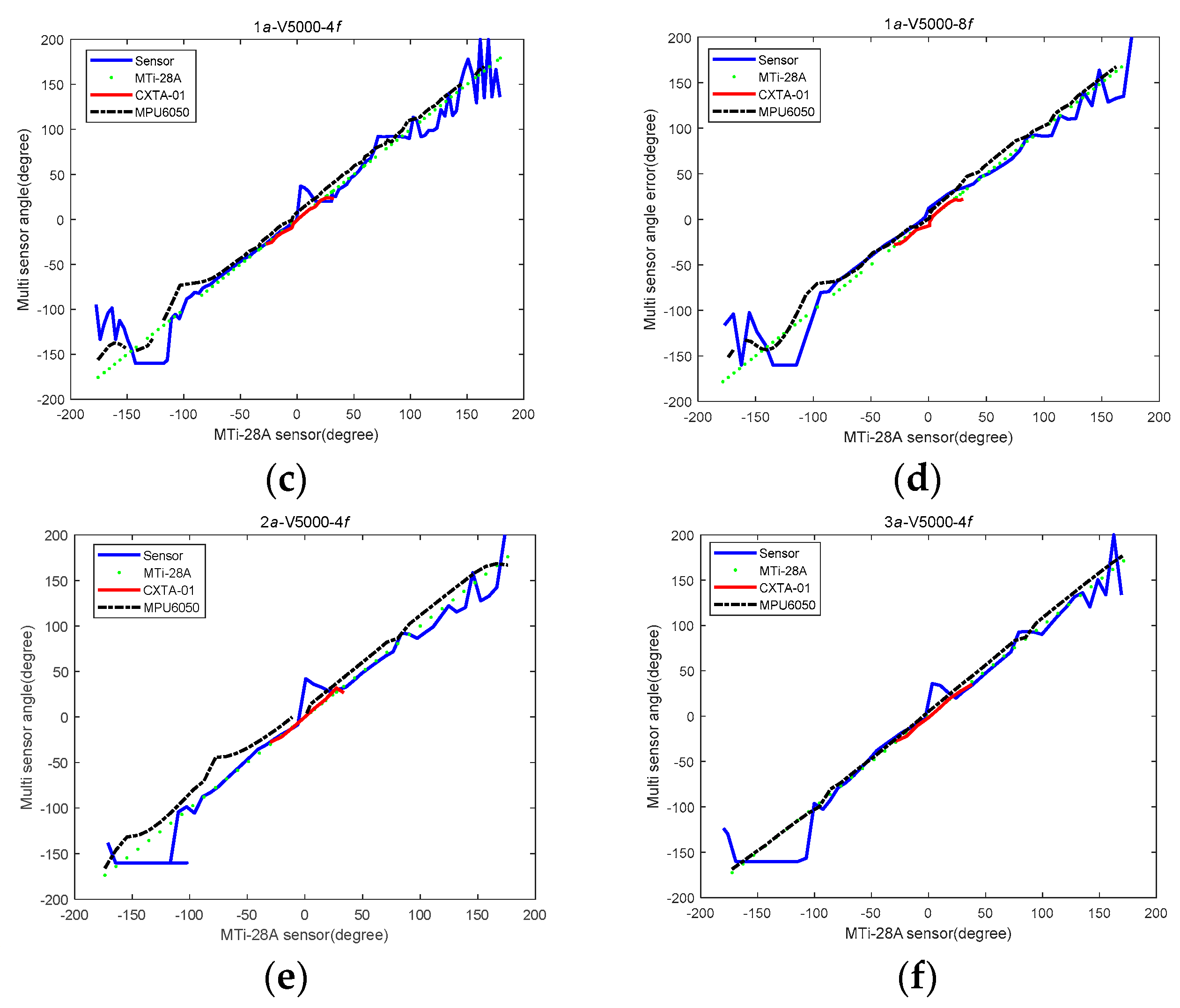
5.3. Experiments of the Sensor Compared with Three Other Sensors
5.4. Key Influencing Factors
- (a)
- The larger the volume of the damping plate is within the allowable range of the structure, the greater the buoyancy obtained.
- (b)
- The density distribution of the damping plate also affects the dynamic characteristics of the sensor. It determines both distance lG and lB, which affect the gravity torque and the buoyancy torque of the damping board, respectively. The larger the values of those two distances, the better the anti-interference ability of the sensor for translational noise.
- (c)
- The density of liquid damping inside the sensor also affects the dynamic characteristics of the sensor.
- (d)
- The system frequency fosc and 16-bit PCA register of the C8051 single-chip microcomputer that was used to measure the oscillation frequency value of the sensor determine the accuracy of the sensor.
- (1)
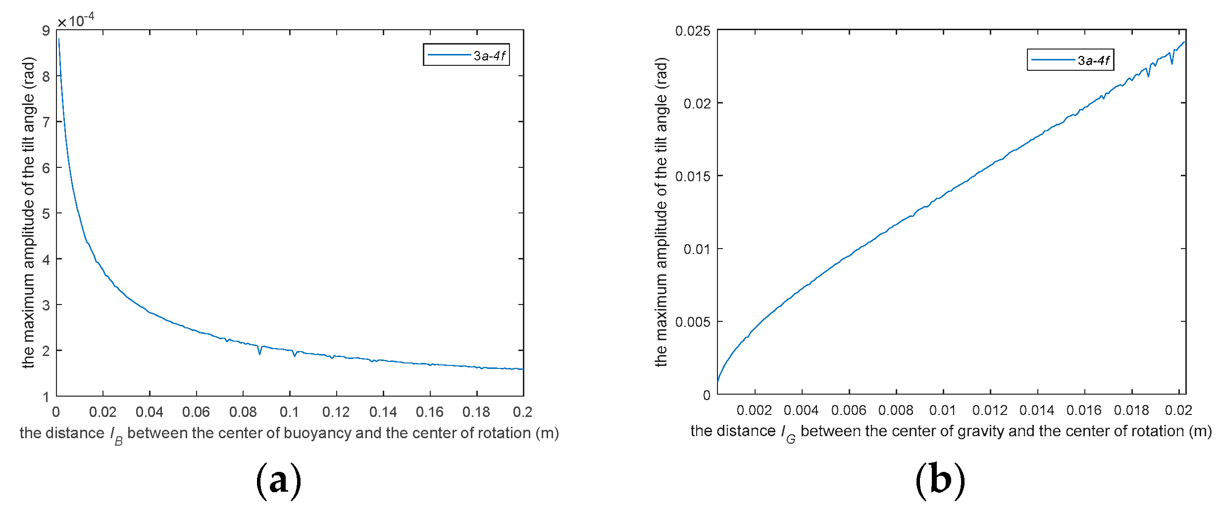
- First, we analyzed the influence of parameter lB on the dynamic characteristics of the sensor. All the parameters except parameter lB were set to a fixed value respectively. We can get an unary function as shown in the Figure 24a below.
- (2)
- Similarly, the influence of parameter lG on the dynamic performance of the sensor is shown in the Figure 24b below.
- (3)
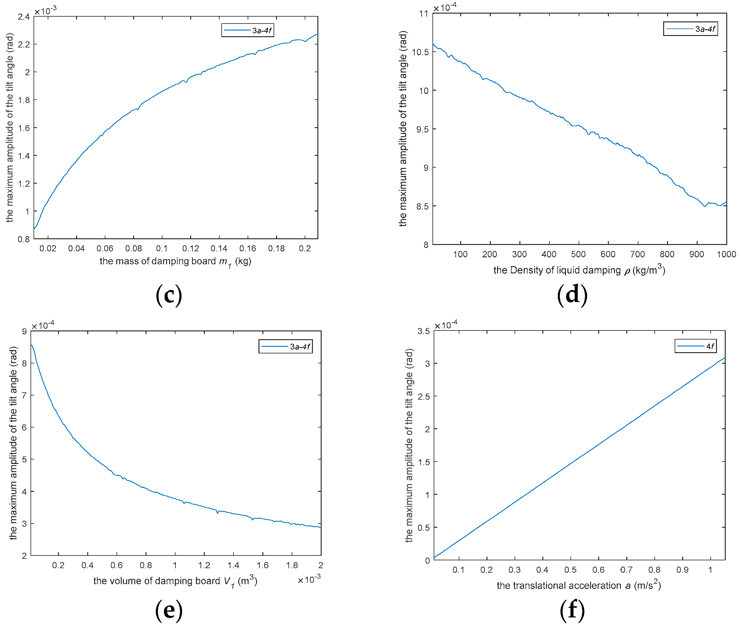
- The influence of the mass m1 of the damping board on the sensor is shown in the Figure 24c below.
- (4)
- The effect of the density of the liquid damping on the characteristics of the sensor is shown in the Figure 24d.
- (5)
- The effect of damper plate volume V1 on sensor characteristics is shown in the Figure 24e.
- (6)
- The influence of translational acceleration a amplitude on sensor characteristics is shown in the Figure 24f.
6. Conclusions
- (1)
- The structure of the dynamic tilt sensor is designed based on an eccentric principle, which has the advantage of a wide measuring range.
- (2)
- The translational noise of the sensor is reduced by the internal damping effect of the liquid with which the sensor is filled.
- (3)
- The translational noise of the sensor is also reduced by a design that places the center of gravity and the center of buoyancy at non-coinciding points.
- (a)
- We will carry out the multi-parameter optimization to refine the parameters of the sensor.
- (b)
- The machining accuracy of sensor structure components needs to be further improved.
- (c)
- The assembly accuracy of sensor structure parts needs to be further improved.
- (d)
- Filtering algorithms should be developed for the sensor to process its output raw data.
- (e)
- Research on the influence of viscosity coefficient on the characteristics of the sensor is needed in the future.
- (f)
- Our own sensor calibration platform is not precise enough, there are calibration errors.
Author Contributions
Funding
Conflicts of Interest
Appendix A

| Number | Portion of Gap | Permeance of Portion |
|---|---|---|
| 1 | 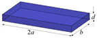 | |
| 2 |  | |
| 3 |  | |
| 4 |  | |
| 5 |  | |
| 6 |  | |
| 7 |  | |
| 8 | 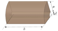 | |
| 9 | 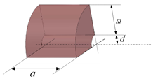 | |
| 10 | 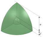 |
Appendix B
References
- Sauter, T.; Nachtnebel, H.; Kero, N. A smart capacitive angle sensor. IEEE Trans. Ind. Inform. 2005, 1, 250–258. [Google Scholar] [CrossRef]
- George, B.; Kumar, V.J. Digital differential capacitive angle transducer. In Proceedings of the 2007 IEEE Instrumentation & Measurement Technology Conference IMTC 2007, Warsaw, Poland, 1–3 May 2007; pp. 1–6. [Google Scholar]
- Thi Thuy, H.T.; Dac, H.N.; Quoc, T.V.; Quoc, T.P.; Ngoc, A.N.; Duc, T.C.; Bui, T.T. Study on design optimization of a capacitive tilt angle sensor. IETE J. Res. 2019, 8, 1–8. [Google Scholar] [CrossRef]
- Chen, D.; Zhang, Z. Deflection Angle Detection of the Rotor and Signal Processing for a Novel Rotational Gyroscope; Springer International Publishing: Cham, Switzerland, 2018. [Google Scholar]
- Zhang, F. Natural convection gas pendulum and its application in accelerometer and tilt senor. Prog. Nat. Sci. 2005, 15, 857–860. [Google Scholar]
- Piao, L.; Zhang, W.; Zhang, F. FEM analysis of the pendulum characteristic of nature convection in dimensional enclosure. Electron. Compon. Mater. 2003, 22, 16–18. [Google Scholar]
- Piao, L.; Piao, R.; Ren, A.; Hu, Y. Research on pendulum characteristic of natural convection gas within three-dimensional closed cavity. In Proceedings of the 2018 IEEE 4th Information Technology and Mechatronics Engineering Conference (ITOEC), Chongqing, China, 14–16 December 2018; IEEE: Piscataway, NJ, USA, 2018; pp. 1703–1707. [Google Scholar]
- Sun, Y.; Di, Q.; Zhang, W.; Chen, W.; Yang, Y.; Zheng, J. Dynamic inclination measurement at-bit based on MEMS accelerometer. In Proceedings of the 2017 29th Chinese Control and Decision Conference (CCDC), Chongqing, China, 28–30 May 2017; pp. 5016–5019. [Google Scholar]
- Yao, X.; Sun, G.; Lin, W.Y.; Chou, W.C.; Lei, K.F.; Lee, M.Y. The design of an In-Line accelerometer-based inclination sensing system. In Proceedings of the 2012 IEEE International Symposium on Circuits and Systems (ISCAS), Seoul, Korea, 20–23 May 2012; IEEE: Piscataway, NJ, USA; pp. 333–336. [Google Scholar]
- Duan, X.; Liu, J.; Li, J.; Yang, W.; Xian, H. Design of digital dipmeter based on MEMS accelerometer and SOC MCU. In Proceedings of the 2011 Fourth International Conference on Intelligent Computation Technology and Automation, Shenzhen, China, 28–29 March 2011; IEEE: Piscataway, NJ, USA; pp. 1085–1088. [Google Scholar]
- Yang, R.; Bao, H.; Zhang, S.; Ni, K.; Zheng, Y.; Dong, X. Simultaneous measurement of tilt angle and temperature with pendulum-based fiber Bragg grating sensor. IEEE Sens. J. 2015, 15, 6381–6384. [Google Scholar] [CrossRef]
- Zhang, Q.; Zhu, T.; Yin, F.; Chiang, K.S. Temperature-insensitive real-time inclinometer based on an etched fiber Bragg grating. IEEE Photonics Technol. Lett. 2014, 26, 1049–1052. [Google Scholar] [CrossRef]
- Tang, G.; Wei, J. A fiber Bragg grating based tilt sensor suitable for constant temperature room. J. Opt. 2015, 17, 1–6. [Google Scholar] [CrossRef]
- Jiang, S.; Wang, J.; Sui, Q. Distinguishable circumferential inclined direction tilt sensor based on fiber Bragg grating with wide measuring range and high accuracy. Opt. Commun. 2015, 35, 58–63. [Google Scholar] [CrossRef]
- Wang, Y.; Zhao, C.-L.; Hu, L.; Kang, J.; Dong, X.; Zhang, Z.; Jing, S. A novel tilt sensor with a large measurement range based on long-period fiber grating. In Proceedings of the 2011 International Conference on Electronics and Optoelectronics, Dalian, China, 29–31 July 2011; pp. V465–V467. [Google Scholar]
- Bezglasnyi, S.P. Stabilization of stationary motions of a gyrostat with a cavity filled with viscous fluid. Russ. Aeronaut. 2014, 57, 333–338. [Google Scholar] [CrossRef]
- Ji, Q.; Zhang, S.; Zhao, H. Design and implementation of an active pendulum control system for fluid damping measurement. In Proceedings of the 2017 4th International Conference on Information Science and Control Engineering (ICISCE), Changsha, China, 21–23 July 2017; IEEE: Piscataway, NJ, USA; pp. 936–941. [Google Scholar]
- Guo, L.; Liao, Q.; Wei, S. Design of a novel biomimetic tilt sensor based on variable reluctive transducer. In Proceedings of the 9th International Conference on Electronic Measurement and Instruments, Beijing, China, 16–19 August 2009; pp. 1350–1354. [Google Scholar]


| System Parameter | Specification |
|---|---|
| Number of turns(rotation) | 1070 |
| Number of turns(rotation) Number of turns(rotation) Number of turns(rotation & translation) Capacitance parameter C1 Capacitance parameter C2 Capacitance parameter C3 Radius R Radius r a b | 878 657 1030 220 nF 220 nF 10 nF 32 mm 31.5 mm 6 mm 3 mm |
| δ(rotation) δ(rotation & translation) | 0.18 mm 0.44 mm |
| Results of Various a and f | Figure | Title |
|---|---|---|
| 1a V5000 1f 1a V5000 2f 1a V5000 4f 1a V5000 8f 2a V5000 4f | Figure 22a Figure 22b Figure 22c Figure 22d Figure 22e | 1a-V5000-1f 1a-V5000-2f 1a-V5000-4f 1a-V5000-8f 2a-V5000-4f |
| 3a V5000 4f | Figure 22f | 3a-V5000-4f |
© 2019 by the authors. Licensee MDPI, Basel, Switzerland. This article is an open access article distributed under the terms and conditions of the Creative Commons Attribution (CC BY) license (http://creativecommons.org/licenses/by/4.0/).
Share and Cite
Guo, L.; Zhang, L.; Song, Y.; Zhao, L.; Zhao, Q. Design and Implementation of a Novel Tilt Sensor Based on the Principle of Variable Reluctance. Sensors 2019, 19, 5228. https://doi.org/10.3390/s19235228
Guo L, Zhang L, Song Y, Zhao L, Zhao Q. Design and Implementation of a Novel Tilt Sensor Based on the Principle of Variable Reluctance. Sensors. 2019; 19(23):5228. https://doi.org/10.3390/s19235228
Chicago/Turabian StyleGuo, Lei, Lishuai Zhang, Yuan Song, Liang Zhao, and Qiancheng Zhao. 2019. "Design and Implementation of a Novel Tilt Sensor Based on the Principle of Variable Reluctance" Sensors 19, no. 23: 5228. https://doi.org/10.3390/s19235228
APA StyleGuo, L., Zhang, L., Song, Y., Zhao, L., & Zhao, Q. (2019). Design and Implementation of a Novel Tilt Sensor Based on the Principle of Variable Reluctance. Sensors, 19(23), 5228. https://doi.org/10.3390/s19235228