Bayesian Prediction of Pre-Stressed Concrete Bridge Deflection Using Finite Element Analysis


Abstract
:1. Introduction
2. Gaussian Process Regression (GPR)
2.1. Bayesian Inference in GPR
2.2. Covariance Matrix Design Using Kernel Functions
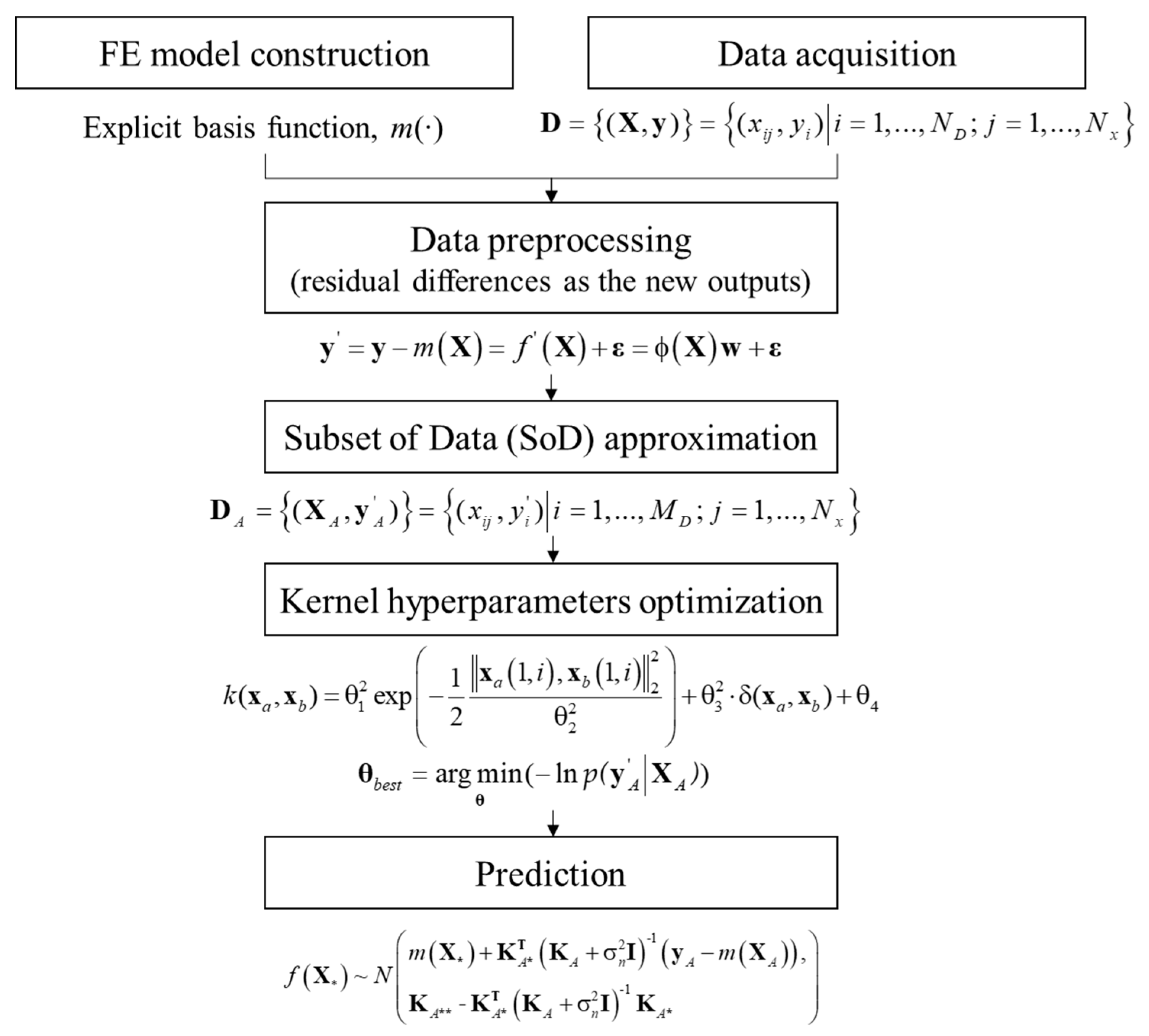
2.3. GPR with FE Analysis Results
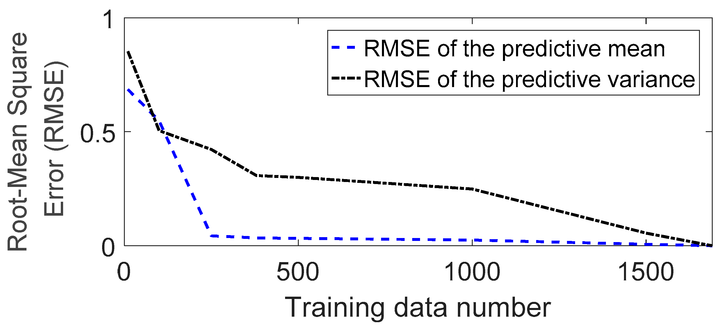
2.4. Approximation Algorithm for Reducing Computational Cost
3. Application Example
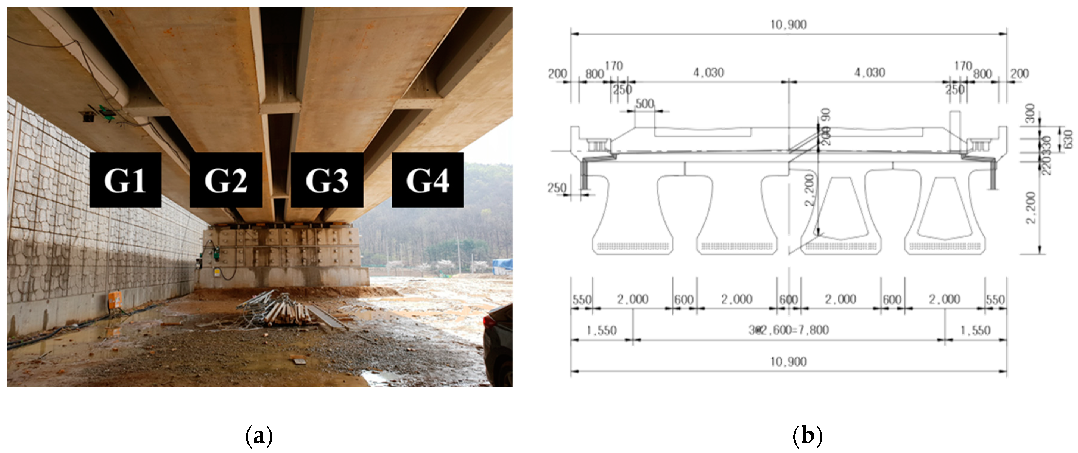
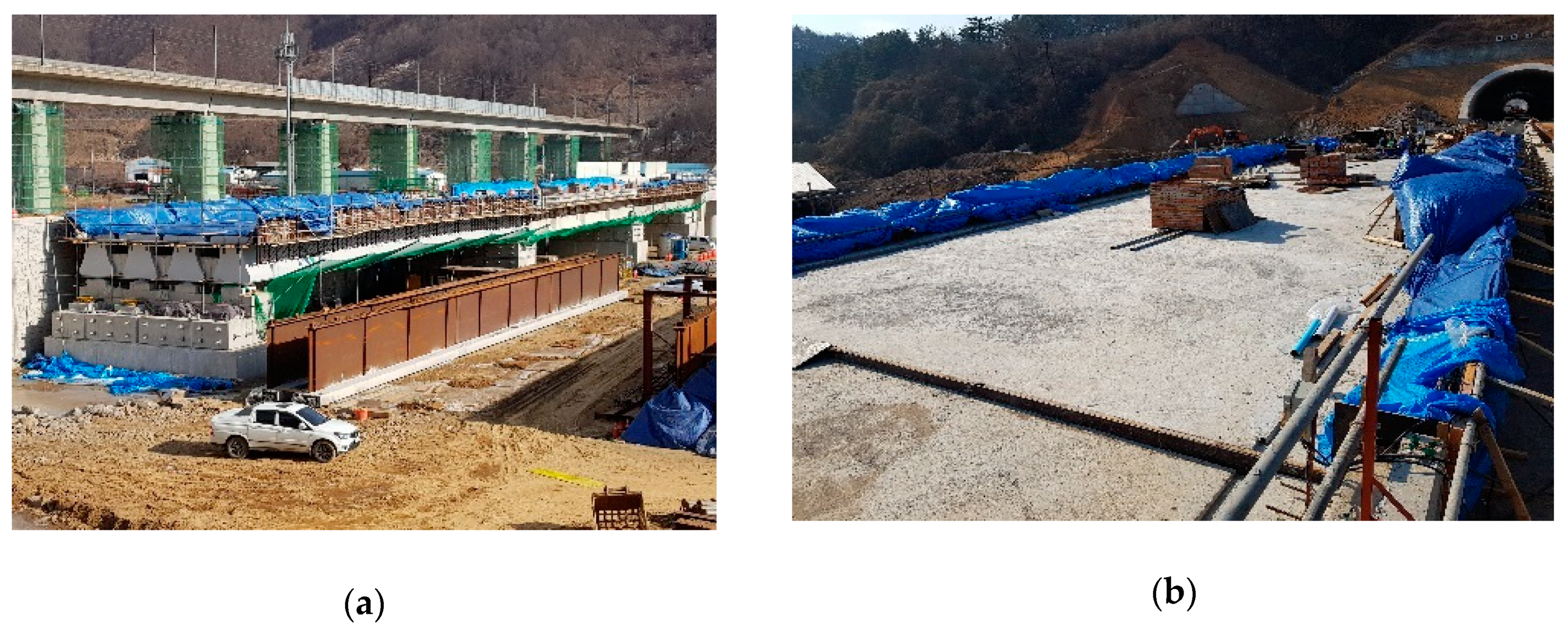
3.1. Example Bridge Description
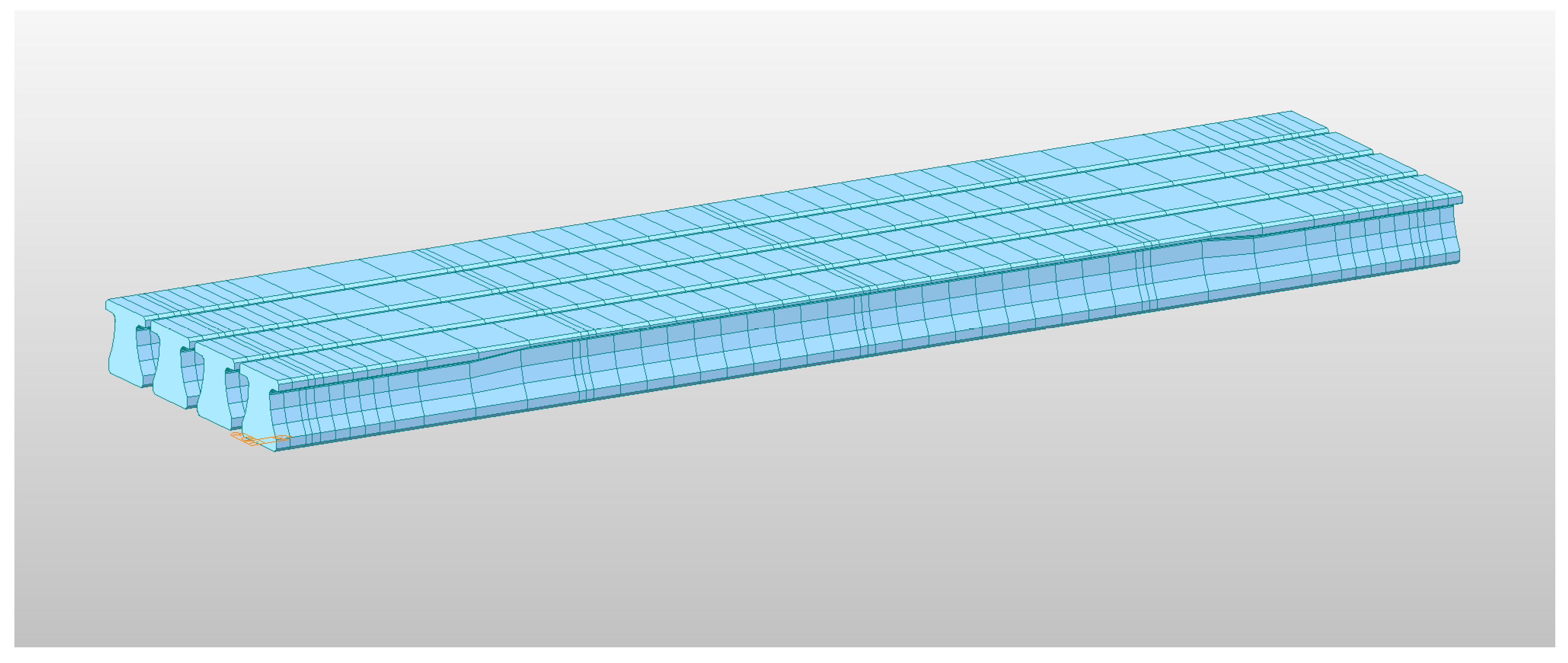
3.2. Prior prediction based on FE analysis
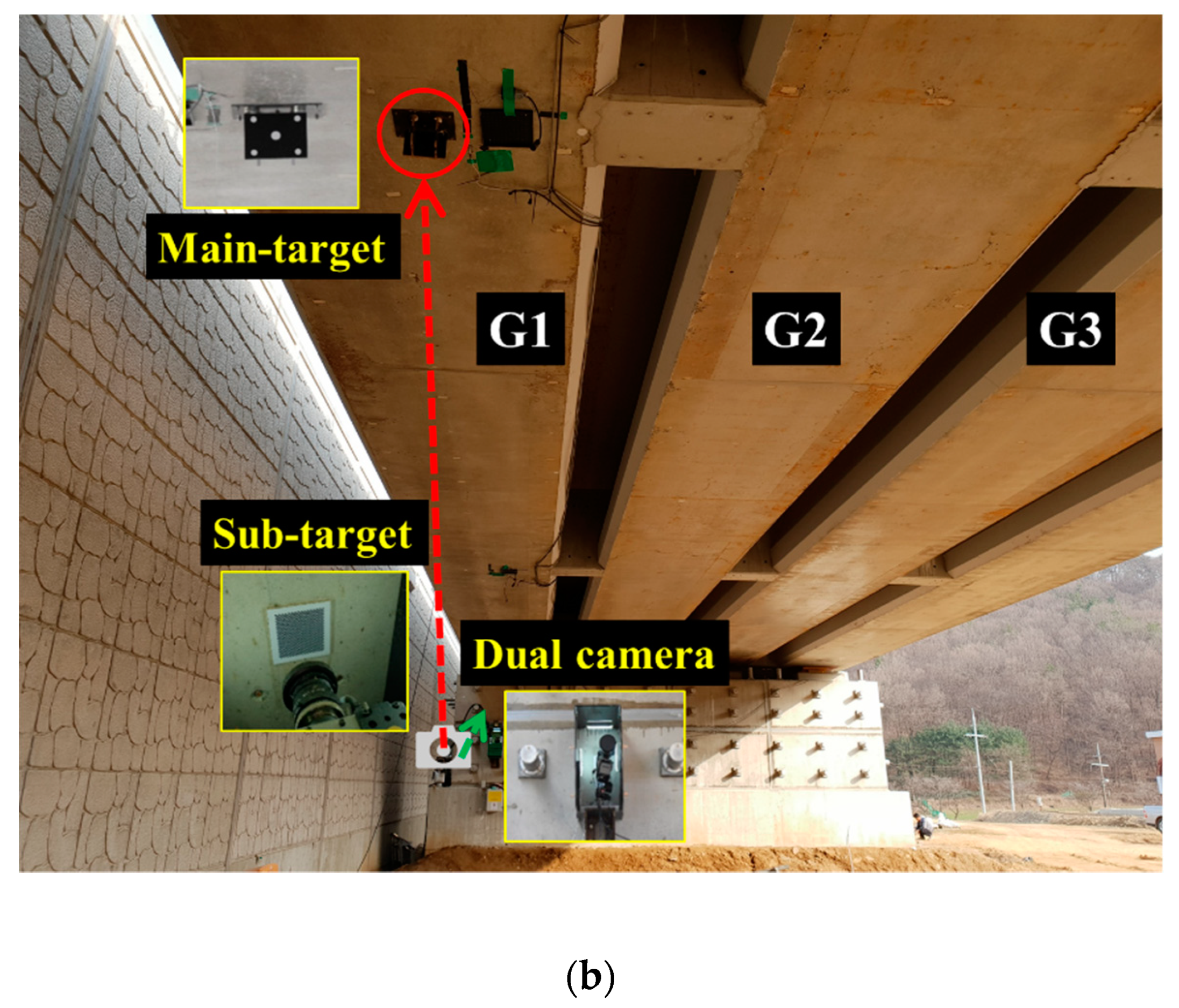
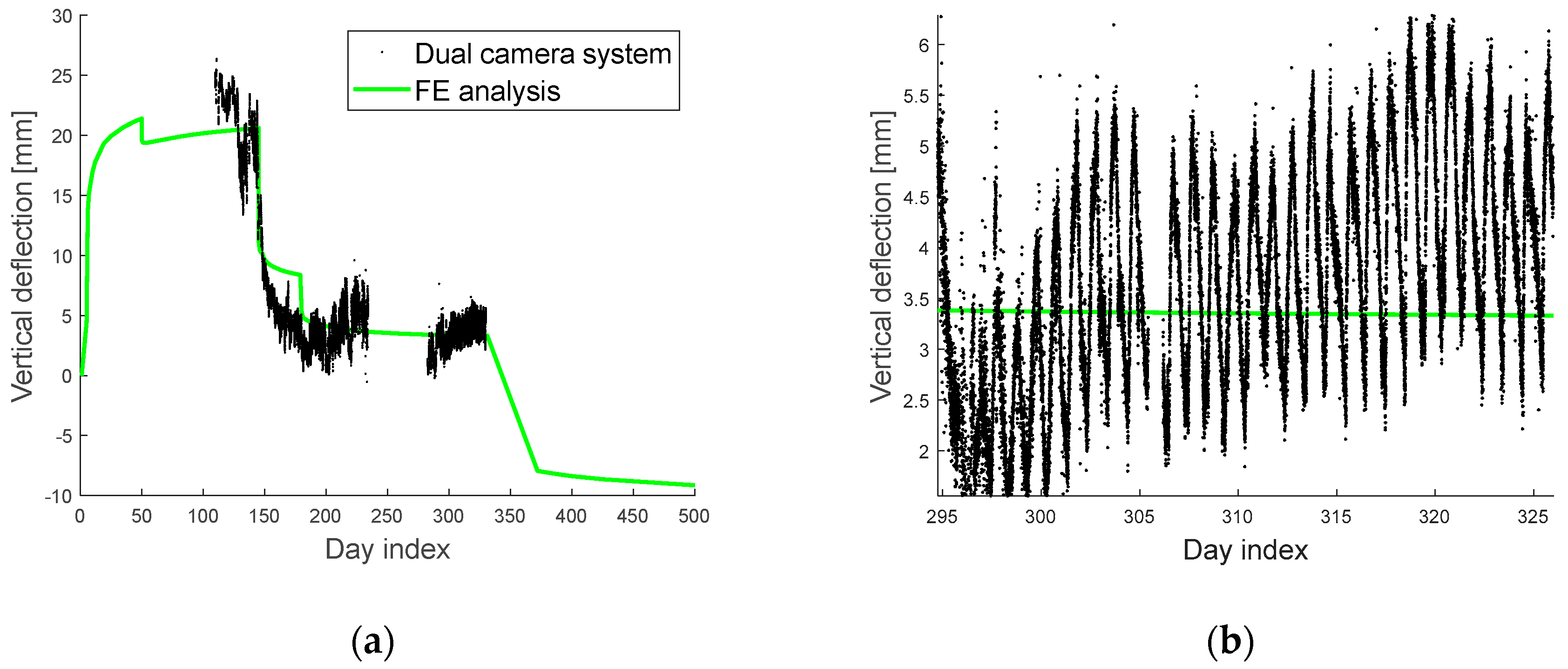
3.3. Measurement Data
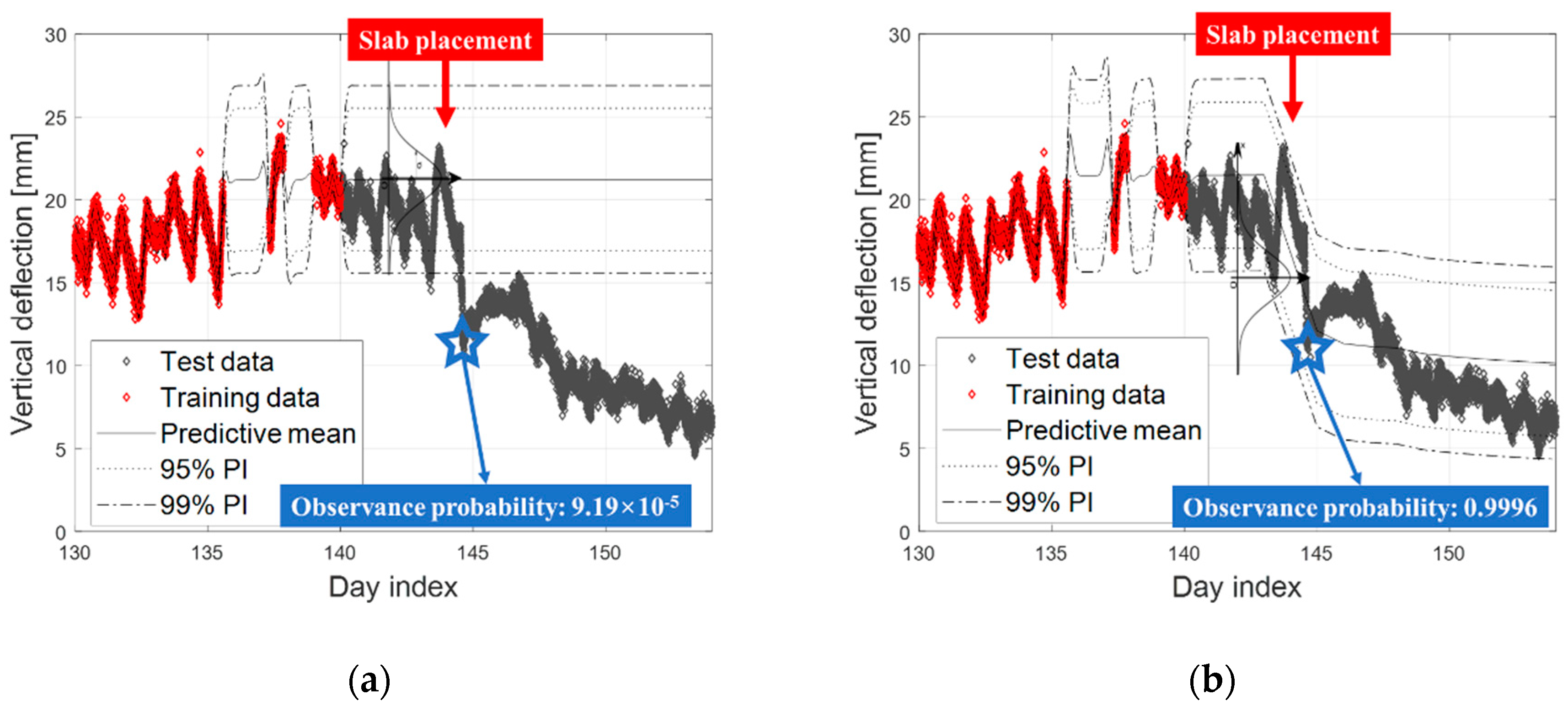
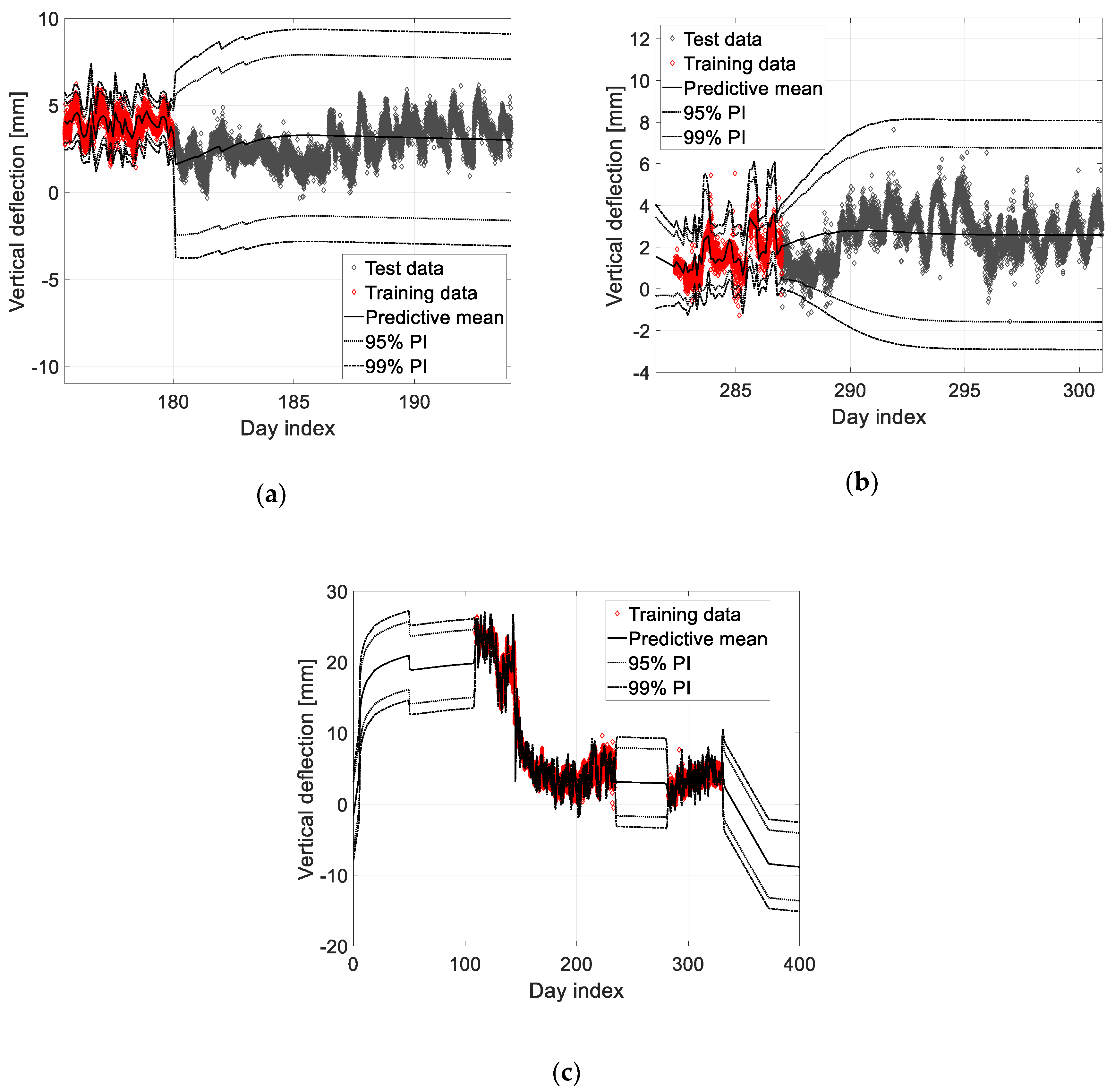
3.4. Probabilistic Prediction Results
4. Conclusions
Author Contributions
Funding
Conflicts of Interest
References
- Guo, T.; Sause, R.; Frangopol, D.M.; Li, A. Time-dependent reliability of PSC box-girder bridge considering creep, shrinkage, and corrosion. J. Bridge Eng. 2010, 16, 29–43. [Google Scholar] [CrossRef]
- Lee, J.; Lee, K.C.; Lee, Y.J. Long-Term Deflection Prediction from Computer Vision-Measured Data History for High-Speed Railway Bridge. Sensors 2018, 18, 1488. [Google Scholar] [CrossRef] [PubMed]
- International Union of Railways (UIC). Testing and Approval of Railway Vehicle from the Point of View of Their Dynamic Behavior-Safety-Track Fatigue-Running behavior; UIC Code 518; UIC: Paris, France, 2009. [Google Scholar]
- Iles, D.C. Design Guide for Steel Railway Bridges; Steel Construction Institute: Berkshire, UK, 2004. [Google Scholar]
- Korea Rail Network Authority. Guideline of Track Maintenance; Korea Rail Network Authority: Daejeon, Korea, 2016. [Google Scholar]
- Guo, T.; Liu, T.; Li, A. Deflection reliability analysis of PSC box-girder bridge under high-speed railway loads. Adv. Struct. Eng. 2012, 15, 2001–2011. [Google Scholar] [CrossRef]
- Nilson, A.H.; Winter, G.; Urquhart, L.C.; Charles Edward, O.R. Design of Concrete Structures; McGraw-Hill: New York, NY, USA, 1991; Volume 49. [Google Scholar]
- Fédération Internationale Du Béton. Structural Concrete: Textbook on Behaviour, Design and Performance; Updated Knowledge of the CEB/FIP Model Code 1990; Bulletin No. 2; FIB: Lausanne, Switzerland, 1999. [Google Scholar]
- Videla, C.; Carreira, D.J.; Garner, N. Guide for modeling and calculating shrinkage and creep in hardened concrete. ACI Rep. 2008, 209.2R–2–209.2R–44. [Google Scholar]
- KCI Committee. Concrete Design Code and Commentary; KCI Committee: Seoul, Korea, 2012. [Google Scholar]
- Bažant, Z.P.; Baweja, S. Creep and shrinkage prediction model for analysis and design of concrete structures: Model B3. ACI Spec. Publ. 2000, 194, 1–84. [Google Scholar]
- Bažant, Z.P.; Yu, Q.; Li, G.H.; Klein, G.J.; Kristek, V. Excessive deflections of record-span prestressed box girder. Concr. Int. 2010, 32, 44–52. [Google Scholar]
- Kamatchi, P.; Rao, K.B.; Dhayalini, B.; Saibabu, S.; Parivallal, S.; Ravisankar, K.; Iyer, N.R. Long-term prestress loss and camber of box-girder bridge. ACI Struct. J. 2014, 111, 1297. [Google Scholar] [CrossRef]
- Bažant, Z.P.; Yu, Q.; Li, G.H. Excessive long-time deflections of prestressed box girders. I: Record-span bridge in Palau and other paradigms. J. Struct. Eng. 2012, 138, 676–686. [Google Scholar] [CrossRef]
- Bažant, Z.P.; Yu, Q.; Li, G.H. Excessive long-time deflections of prestressed box girders. II: Numerical analysis and lessons learned. J. Struct. Eng. 2012, 138, 687–696. [Google Scholar] [CrossRef]
- Sun, L.; Hao, X.W. Analysis of Bridge Deflection Based on Time Series. Appl. Mech. Mater. 2011, 71, 4545–4548. [Google Scholar] [CrossRef]
- Xin, J.; Zhou, J.; Yang, S.; Li, X.; Wang, Y. Bridge structure deformation prediction based on GNSS data using Kalman-ARIMA-GARCH model. Sensors 2018, 18, 298. [Google Scholar] [CrossRef] [PubMed]
- Pnevmatikos, N.G.; Hatzigeorgiou, G.D. Damage detection of framed structures subjected to earthquake excitation using discrete wavelet analysis. Bull. Earthq. Eng. 2017, 15, 227–248. [Google Scholar] [CrossRef]
- Pnevmatikos, N.G.; Blachowski, B.; Hatzigeorgiou, G.D.; Swiercz, A. Wavelet analysis based damage localization in steel frames with bolted connections. Smart Struct. Syst. 2016, 18, 1189–1202. [Google Scholar] [CrossRef]
- Liu, J.L.; Wang, Z.C.; Ren, W.X.; Li, X.X. Structural time-varying damage detection using synchrosqueezing wavelet transform. Smart Struct. Syst. 2015, 15, 119–133. [Google Scholar] [CrossRef]
- Wang, C.; Ren, W.X.; Wang, Z.C.; Zhu, H.P. Time-varying physical parameter identification of shear type structures based on discrete wavelet transform. Smart Struct. Syst. 2014, 14, 831–845. [Google Scholar] [CrossRef]
- Law, S.S.; Zhu, X.Q.; Tian, Y.J.; Li, X.Y.; Wu, S.Q. Statistical damage classification method based on wavelet packet analysis. Struct. Eng. Mech. 2013, 46, 459–486. [Google Scholar] [CrossRef]
- Fan, Z.; Feng, X.; Zhou, J. A novel transmissibility concept based on wavelet transform for structural damage detection. Smart Struct. Syst. 2013, 12, 291–308. [Google Scholar] [CrossRef]
- Yang, I.H. Prediction of time-dependent effects in concrete structures using early measurement data. Eng. Struct. 2007, 29, 2701–2710. [Google Scholar] [CrossRef]
- Guo, T.; Chen, Z. Deflection control of long-span PSC box-girder bridge based on field monitoring and probabilistic FEA. J. Perform. Constr. Facil. 2016, 30, 04016053. [Google Scholar] [CrossRef]
- Lee, Y.J.; Kim, R.; Suh, W.; Park, K. Probabilistic fatigue life updating for railway bridges based on local inspection and repair. Sensors 2017, 17, 936. [Google Scholar] [CrossRef]
- Kim, R.E.; Moreu, F.; Spencer, B.F. System identification of an in-service railroad bridge using wireless smart sensors. Smart Struct. Syst. 2015, 15, 683–698. [Google Scholar] [CrossRef]
- Moreu, F.; Kim, R.E.; Spencer, B.F., Jr. Railroad bridge monitoring using wireless smart sensors. Struct. Control Health Monit. 2017, 24, e1863. [Google Scholar] [CrossRef]
- Kim, R.E.; Moreu, F.; Spencer, B.F., Jr. Hybrid model for railroad bridge dynamics. J. Struct. Eng. 2016, 142, 04016066. [Google Scholar] [CrossRef]
- He, W.Y.; Zhu, S. Adaptive-scale damage detection strategy for plate structures based on wavelet finite element model. Struct. Eng. Mech. 2015, 45, 239–256. [Google Scholar] [CrossRef]
- Rasmussen, C.E.; Williams, C.K. Gaussian Processes for Machine Learning; MIT Press: Cambridge, MA, USA, 2006. [Google Scholar]
- Barber, D. Bayesian Reasoning and Machine Learning; Cambridge University Press: Cambridge, UK, 2012. [Google Scholar]
- Hager, W.W. Updating the inverse of a matrix. SIAM Rev. 1989, 31, 221–239. [Google Scholar] [CrossRef]
- Snelson, E.L. Flexible and Efficient Gaussian Process Models for Machine Learning. Ph.D. Thesis, University College London (UCL), London, UK, 2007. [Google Scholar]
- Chalupka, K.; Williams, C.K.; Murray, I. A framework for evaluating approximation methods for Gaussian process regression. J. Mach. Learn. Res. 2013, 14, 333–350. [Google Scholar]
- Liu, H.; Ong, Y.S.; Shen, X.; Cai, J. When Gaussian process meets big data: A review of scalable GPs. arXiv 2018, arXiv:1807.01065. [Google Scholar]
- Herbrich, R.; Lawrence, N.D.; Seeger, M. Fast sparse Gaussian process methods: The informative vector machine. In Proceedings of the 15th International Conference on Neural Information Processing Systems; MIT Press: Cambridge, MA, USA, 2002; pp. 625–632. [Google Scholar]
- Keerthi, S.; Chu, W. A matching pursuit approach to sparse gaussian process regression. In Proceedings of the 18th International Conference on Neural Information Processing Systems; MIT Press: Vancouver, BC, Canada, 2006; pp. 643–650. [Google Scholar]
- Seeger, M. Bayesian Gaussian Process Models: PAC-Bayesian Generalisation Error Bounds and Sparse Approximations; No. THESIS_LIB; University of Edinburgh: Edinburgh, UK, 2003. [Google Scholar]
- Lee, J.; Lee, K.C.; Kwon, H.C.; Lim, K.M.; Min, K.H. Long-term Behavior of Pretension Girder Bridges by Construction Phase Time. J. Korean Soc. Hazard Mitig. 2018, 18, 51–56. [Google Scholar] [CrossRef]
- Midas Civil 2017 [Computer Software]; MIDAS Engineering Software: Seongnam, Korea, 2017.
- Lee, J.; Lee, K.C.; Jeong, S.; Lee, Y.J.; Sim, S.H. Long-term displacement of full-scale bridges using camera ego-motion compensation. Mechanical Systems and Signal Processing, Under Review. 2019. [Google Scholar]


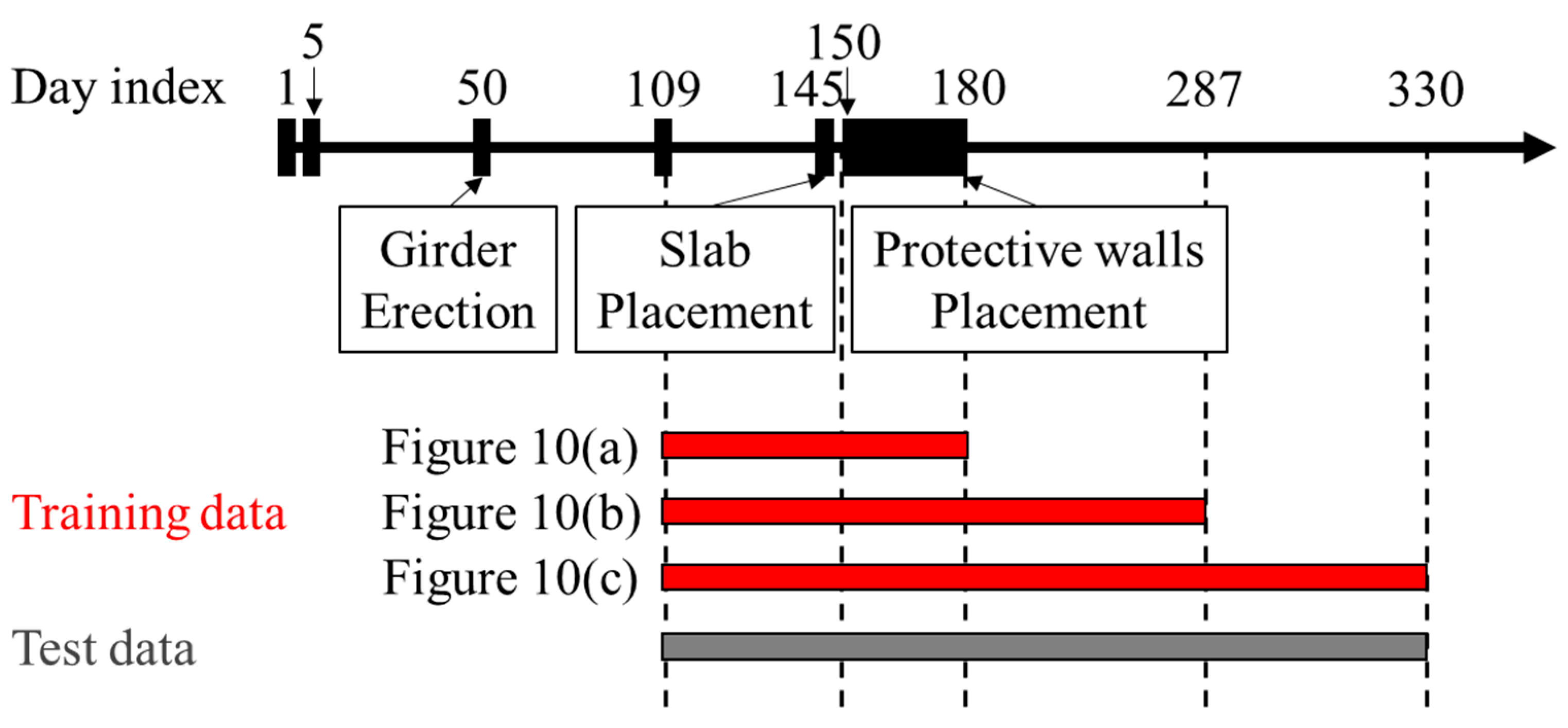
| Date | Day Index | Construction Schedule |
|---|---|---|
| 18 September 2017 | 1 | Girder concrete casting and tendon tensioning |
| 22 September 2017 | 5 | Tendon release |
| 6 November 2017 | 50 | Girder erection |
| 8–9 February 2018 | 144–145 | Slab placement |
| 14 February 2018–16 March 2018 | 150–180 | Protective wall placement |
| Classification | Concrete | ||
|---|---|---|---|
| Slab | Cross Beam | Girder | |
| Material code in MIDAS | C30 | C30 | C49 |
| Compressive strength | 30 MPa | 30 MPa | 49 MPa |
| Modulus of elasticity | 27.52 GPa | 27.52 GPa | 32.08 GPa |
| Unit weight | 2.5 ton/m3 | 2.5 ton/m3 | 2.5 ton/m3 |
| Poisson’s ratio | 0.18 | 0.18 | 0.18 |
| Classification | Strand |
|---|---|
| Material code in MIDAS | SWPC7B 15.2 mm, Low Relaxation |
| Modulus of elasticity | 200,000 MPa |
| Unit weight | 7.85 ton/m3 |
| Poisson’s ratio | 0.3 |
| Total tendon area | 15.2 mm × 90 EA |
| Ultimate strength | 1900 MPa |
| Yield strength | 1600 MPa |
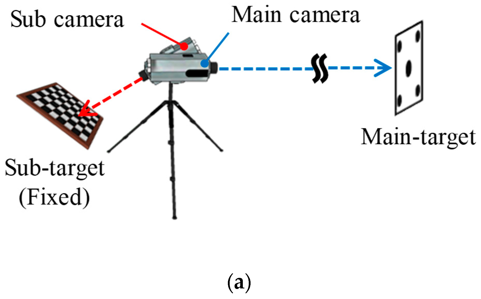
| Item | Specifications |
|---|---|
| Main camera | Telescope lens (focal length: 800 mm) 1920 × 1200 resolution |
| Sub-camera | Wide-angle lens (focal length: 6 mm) 1920 × 1200 resolution |
| Main target | Five circular dots 15 × 11 cm2 |
| Sub-target | 32 × 31 checkerboard |
© 2019 by the authors. Licensee MDPI, Basel, Switzerland. This article is an open access article distributed under the terms and conditions of the Creative Commons Attribution (CC BY) license (http://creativecommons.org/licenses/by/4.0/).
Share and Cite
Lee, J.; Lee, K.-C.; Sim, S.-H.; Lee, J.; Lee, Y.-J. Bayesian Prediction of Pre-Stressed Concrete Bridge Deflection Using Finite Element Analysis. Sensors 2019, 19, 4956. https://doi.org/10.3390/s19224956
Lee J, Lee K-C, Sim S-H, Lee J, Lee Y-J. Bayesian Prediction of Pre-Stressed Concrete Bridge Deflection Using Finite Element Analysis. Sensors. 2019; 19(22):4956. https://doi.org/10.3390/s19224956
Chicago/Turabian StyleLee, Jaebeom, Kyoung-Chan Lee, Sung-Han Sim, Junhwa Lee, and Young-Joo Lee. 2019. "Bayesian Prediction of Pre-Stressed Concrete Bridge Deflection Using Finite Element Analysis" Sensors 19, no. 22: 4956. https://doi.org/10.3390/s19224956
APA StyleLee, J., Lee, K.-C., Sim, S.-H., Lee, J., & Lee, Y.-J. (2019). Bayesian Prediction of Pre-Stressed Concrete Bridge Deflection Using Finite Element Analysis. Sensors, 19(22), 4956. https://doi.org/10.3390/s19224956