Data Anomaly Detection for Internet of Vehicles Based on Traffic Cellular Automata and Driving Style


Abstract
:1. Introduction
2. Relative Works
2.1. Traffic Flow Model
2.2. Data Anomaly Detection
3. Model and Description
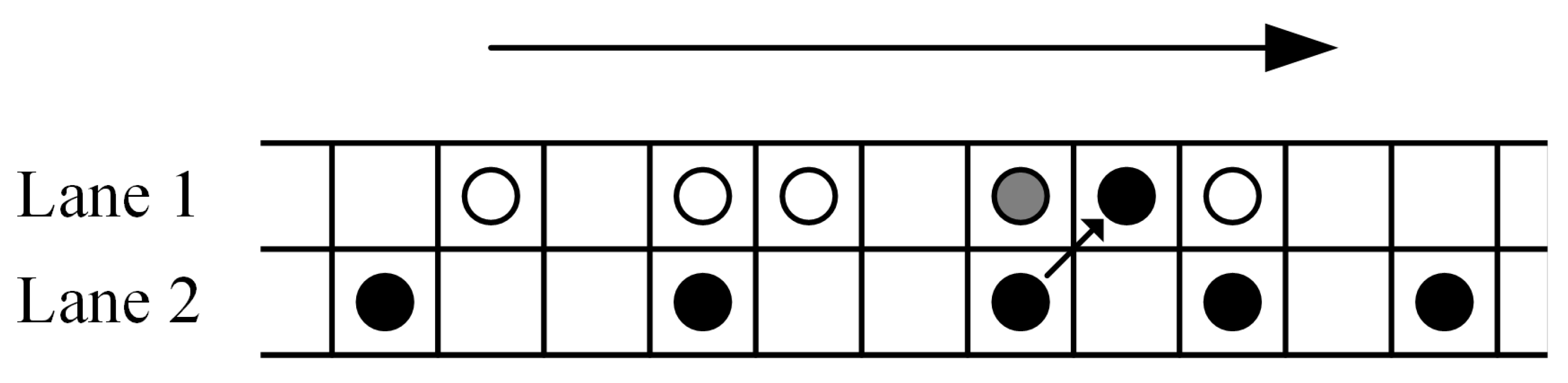
3.1. Traffic Cellular Automata
3.2. Rule Set of Traffic Cellular Automata
3.2.1. Accelerate Rule
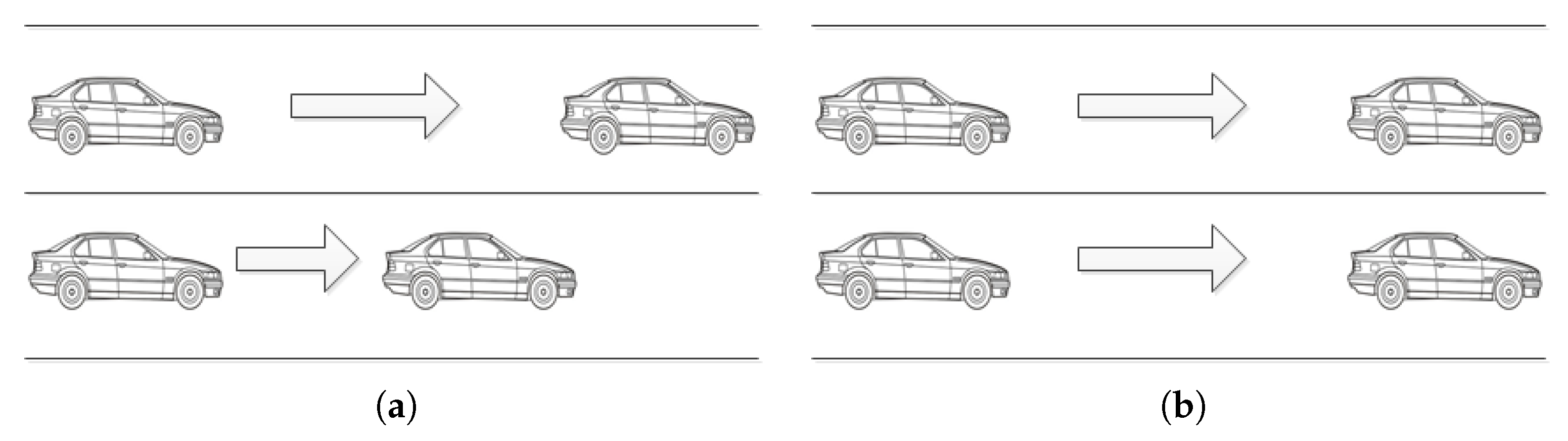
3.2.2. Overtaking/Lane-Changing Rule
3.2.3. Mandatory Deceleration Rule
3.2.4. Random Slowing Rule
3.3. Driving Style Quantization Model
4. Add Algorithm: Anomaly Detection Based on Driving Style
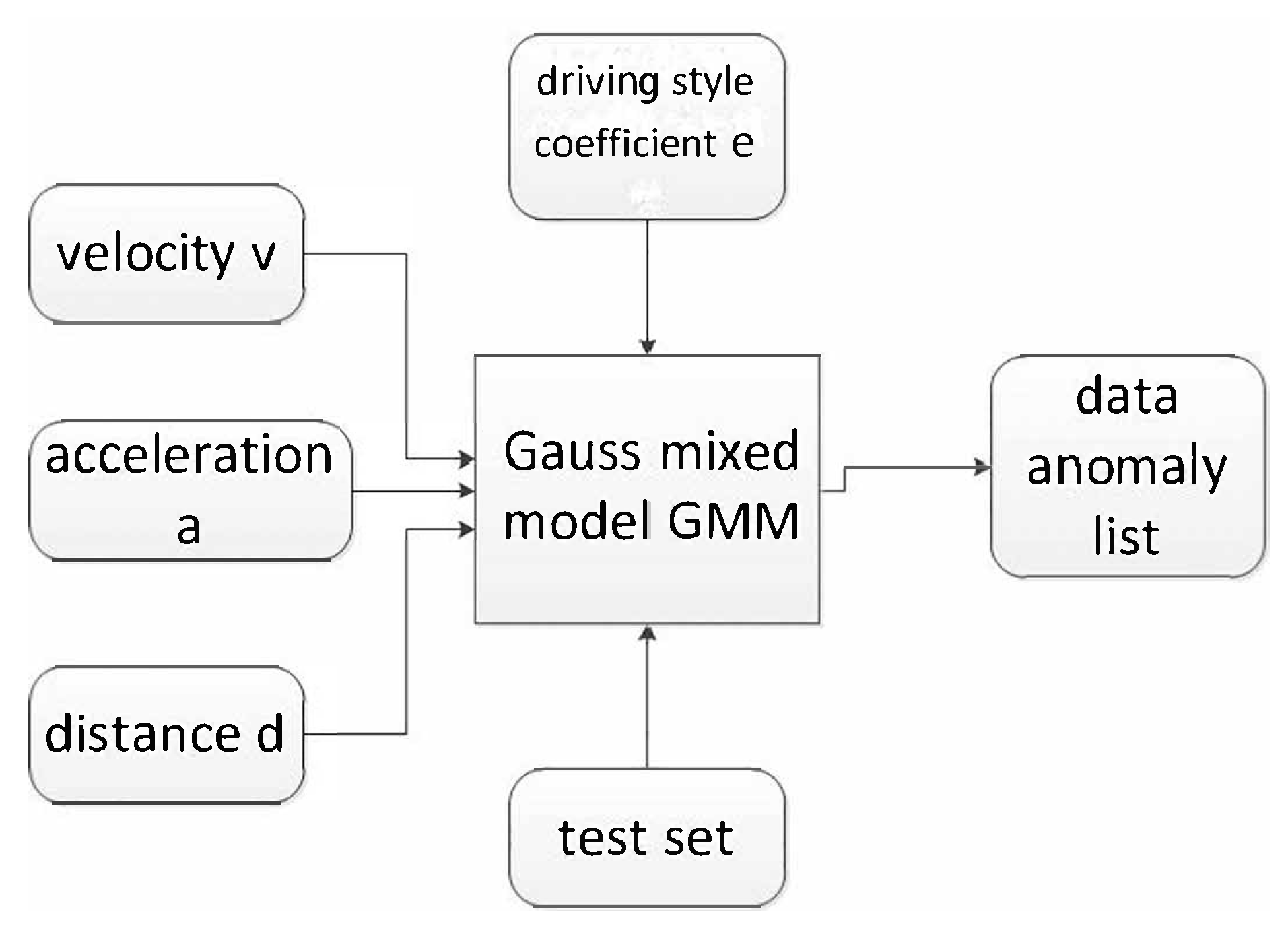
4.1. Gaussian Mixed Model (GMM)
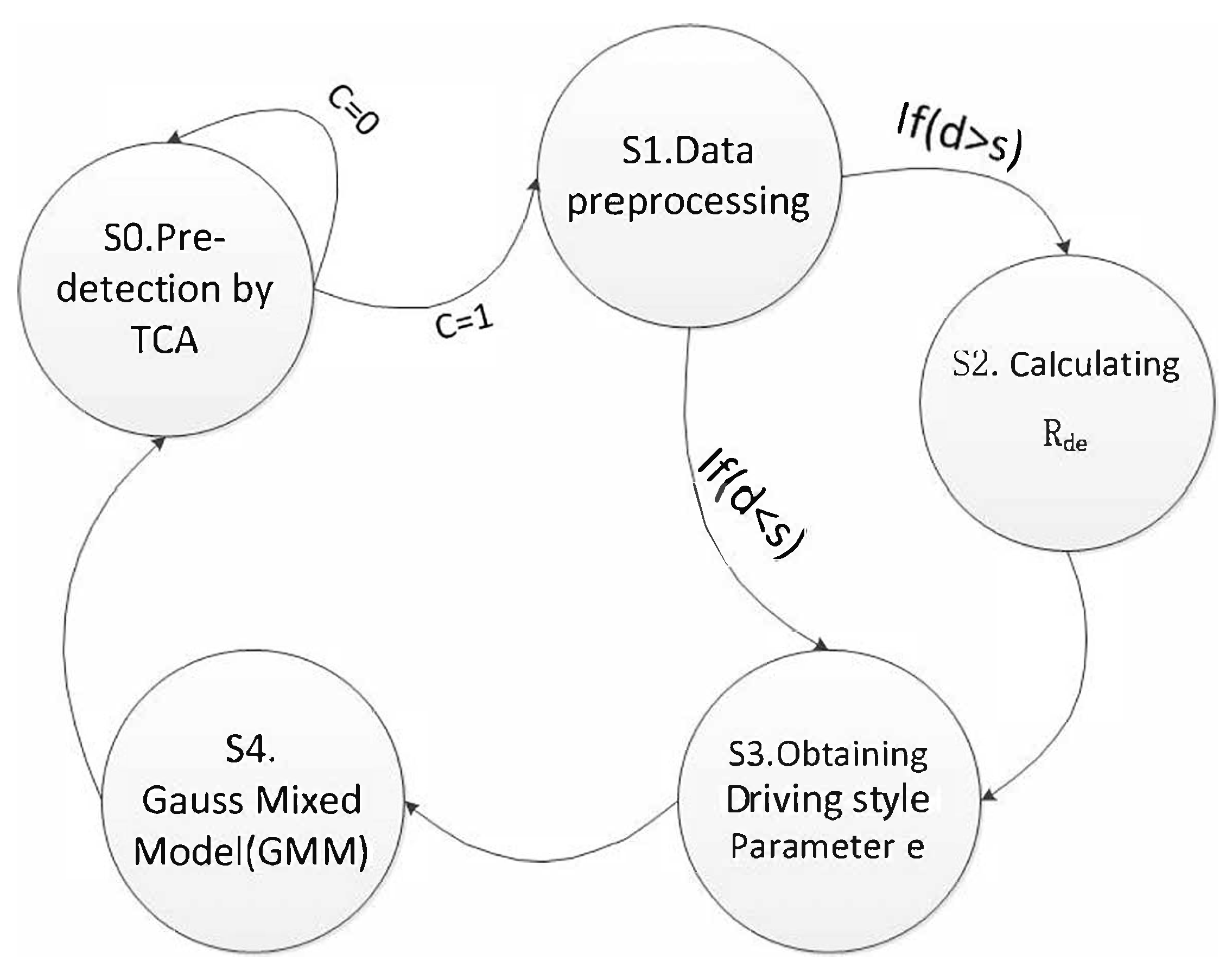
4.2. Add Algorithm
5. Experiment and Analysis
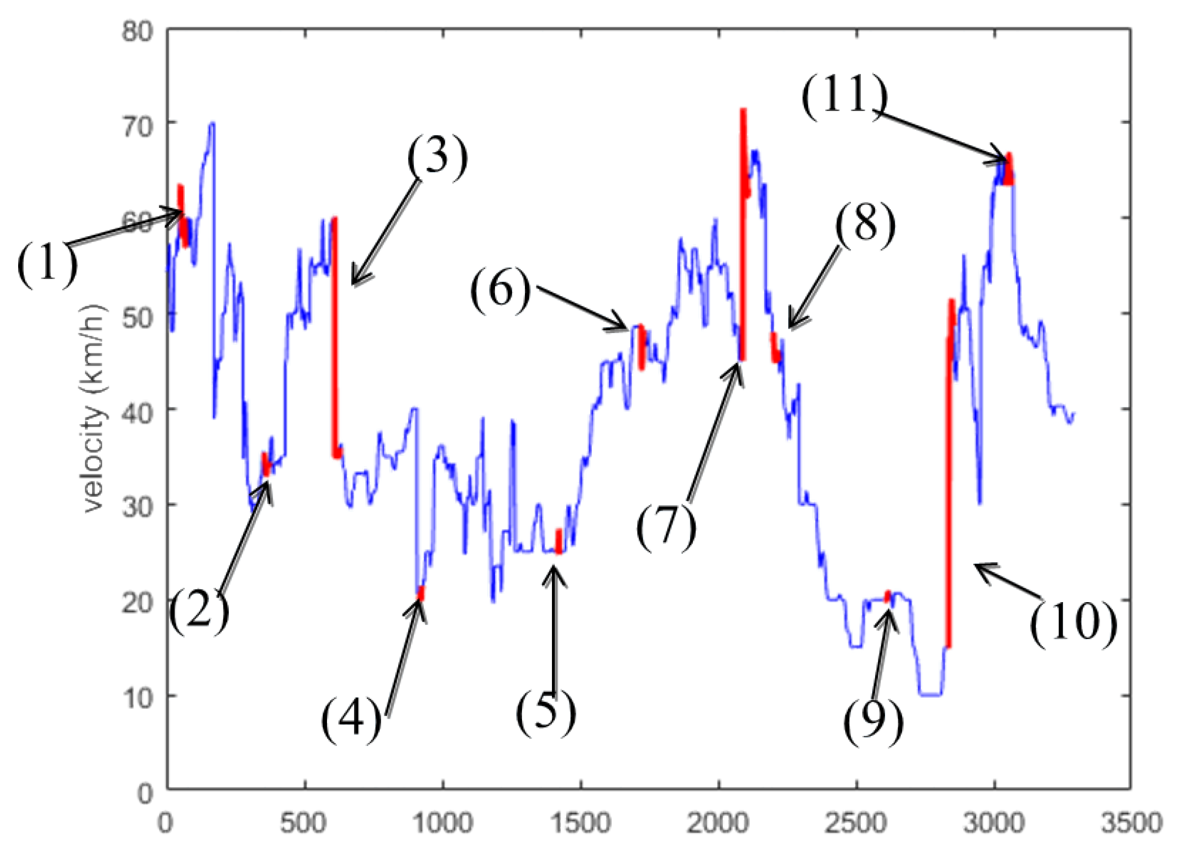
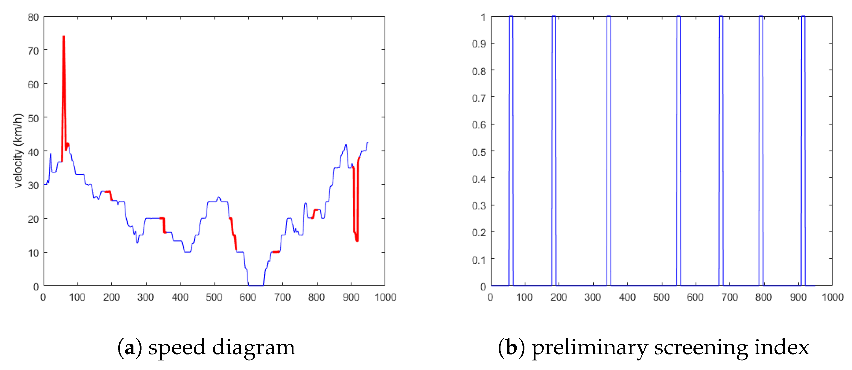
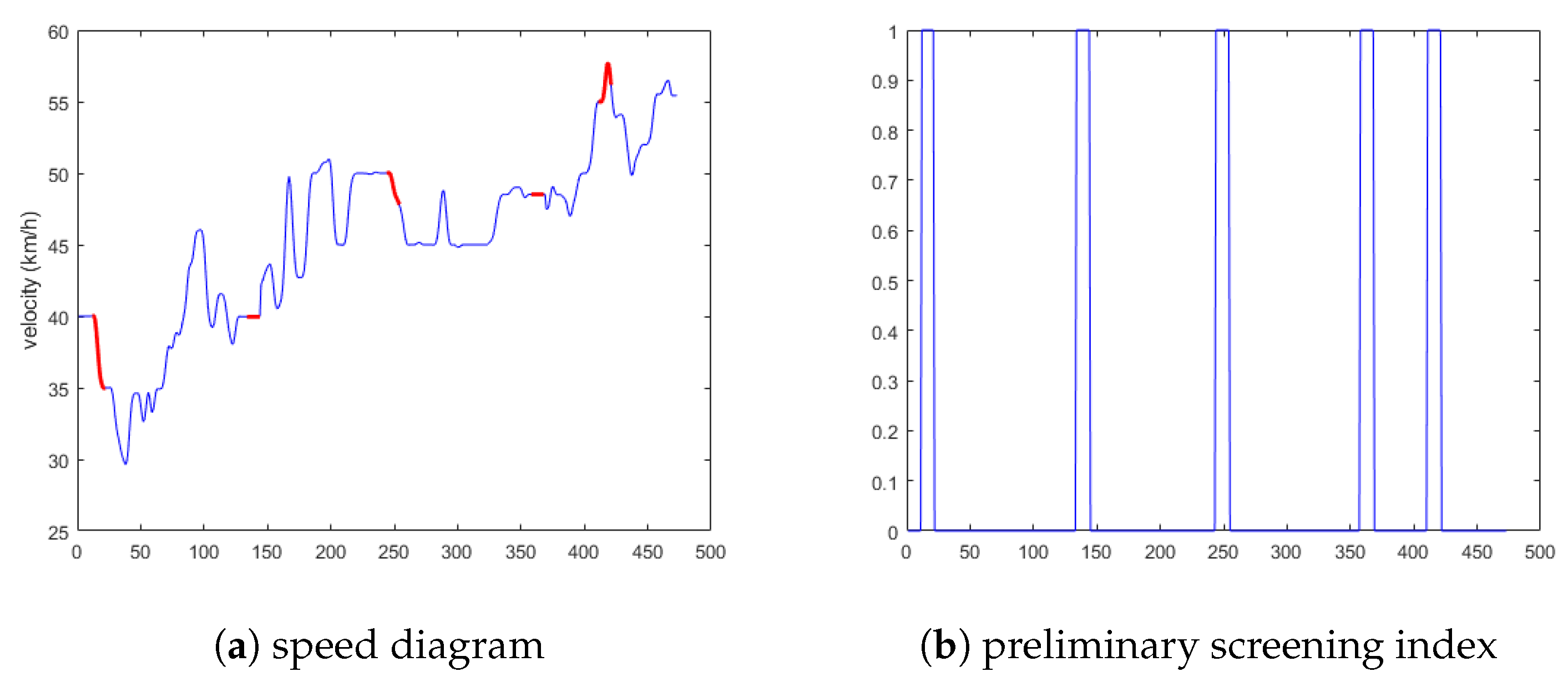
5.1. Experimental Results and Analysis
5.1.1. Experimental Results Analysis of the First Situation
5.1.2. Experimental Results Analysis of the Second Situation
5.1.3. Experimental Results Analysis of the Third Situation
6. Conclusions
Author Contributions
Funding
Acknowledgments
Conflicts of Interest
References
- Ding, N.; Ma, H.; Zhao, C.; Ma, Y.; Ge, H. Driver Emotional State Based-Data Anomaly Detection for Vehicular Ad Hoc Networks. In Proceedings of the IEEE SmartIot, Tianjin, China, 9–11 August 2019. [Google Scholar]
- Ahmed, E.; Gharavi, H. Cooperative vehicular networking: A survey. IEEE Trans. Intell. Transp. Syst. 2018, 19, 996–1014. [Google Scholar] [CrossRef] [PubMed]
- Qiu, T.; Liu, J.; Si, W.; Wu, D.O. Robustness Optimization Scheme With Multi-Population Co-Evolution for Scale-Free Wireless Sensor Networks. IEEE/ACM Trans. Netw. 2019, 27, 1028–1042. [Google Scholar] [CrossRef]
- GCN, Connected Cars Can Lie–Posing a New Threat to Smart Cities. 2018. Available online: https:gcn.comarticles20180613/connected-cars-malicious.aspx (accessed on 1 October 2019).
- Xu, C.; Zhao, F.; Guan, J.; Zhang, H.; Muntean, G.M. Qoe-drivenuser-centric vod services in urban multihomed p2p–based vehicular networks. IEEE Trans. Veh. Technol. 2013, 62, 2273–2289. [Google Scholar] [CrossRef]
- Wang, L.; Da, X.L.; Bi, Z.; Xu, Y. Data cleaning for RFID and WSN integration. IEEE Trans. Ind. Inf. 2013, 10, 408–418. [Google Scholar] [CrossRef]
- Klauer, S.G.; Dingus, T.A.; Neale, V.L.; Sudweeks, J.D.; Ramsey, D.J. The impact of driver inattention on near-crash/crash risk: An analysis using the 100-car naturalistic driving study data. United States. In A Human Factors Evaluation of the Spatial Gesture Interface for In-Vehicle Information Systems; National Highway Traffic Safety Administration: Washington, DC, USA, 2006. [Google Scholar]
- Karagiannis, G.; Altintas, O.; Ekici, E.; Heijenk, G.; Jarupan, B.; Lin, K.; Weil, T. Vehicular networking: A survey and tutorial on requirements, architectures, challenges, standards and solutions. IEEE Commun. Surv. Tutor. 2011, 13, 584–616. [Google Scholar] [CrossRef]
- Jinna, H.; Qiu, T.; Atiquzzaman, M.; Ren, Z. CVCG: Cooperative V2V-aided transmission scheme based on coalitional game for popular content distribution in vehicular ad-hoc networks. IEEE Trans. Mob. Comput. 2018. [Google Scholar] [CrossRef]
- Del Castillo, J.M.; Benitez, F.G. On the functional form of the speed-density relationship—I: General theory. Transp. Res. Part B Methodol. 1995, 29, 373–389. [Google Scholar] [CrossRef]
- Yu, H.; Wu, Z.; Wang, S.; Wang, Y.; Ma, X. Spatiotemporal recurrent convolutional networks for traffic prediction in transportation networks. Sensors 2017, 17, 1501. [Google Scholar] [CrossRef] [PubMed]
- Lighthill, M.J.; Whitham, G.B. On kinematic waves II. A theory of traffic flow on long crowded roads. Proc. R. Soc. Lond. Ser. A Math. Phys. Sci. 1955, 229, 317–345. [Google Scholar]
- Li, L.; Su, X.; Zhang, Y.; Lin, Y.; Li, Z. Trend modeling for traffic time series analysis: An integrated study. IEEE Trans. Intell. Transp. Syst. 2015, 16, 3430–3439. [Google Scholar] [CrossRef]
- Prigogine, I.; Herman, R. Kinetic Theory of Vehicular Traffic: Comparison with Data. Transp. Sci. 1972, 6, 440–452. [Google Scholar]
- Diao, X.; Chen, C.H. A sequence model for air traffic flow management rerouting problem. Transp. Res. Part E Logist. Transp. Rev. 2018, 110, 15–30. [Google Scholar] [CrossRef]
- Khan, Z.H.; Gulliver, T.A. A macroscopic traffic model for traffic flow harmonization. Eur. Transp. Res. Rev. 2018, 10, 30. [Google Scholar] [CrossRef]
- Zhao, H.T.; Yang, S.; Chen, X.X. Cellular automata model for urban road traffic flow considering pedestrian crossing street. Phys. A Stat. Mech. Appl. 2016, 462, 1301–1313. [Google Scholar] [CrossRef]
- Bouadi, M.; Jetto, K.; Benyoussef, A.; El Kenz, A. The investigation of the reentrance phenomenon in cellular automaton traffic flow model. Phys. A Stat. Mech. Appl. 2017, 469, 1–14. [Google Scholar] [CrossRef]
- Lin, C.W.; Sangiovanni-Vincentelli, A. Cyber-security for the controller area network (CAN) communication protocol. In Proceedings of the 2012 International Conference on Cyber Security, Washington, DC, USA, 14–16 December 2012; pp. 1–7. [Google Scholar]
- Müter, M.; Groll, A.; Freiling, F.C. A structured approach to anomaly detection for in-vehicle networks. In Proceedings of the 2010 Sixth International Conference on Information Assurance and Security, Atlanta, GA, USA, 23–25 August 2010; pp. 92–98. [Google Scholar]
- Volkovs, M.; Chiang, F.; Szlichta, J.; Miller, R.J. Continuous data cleaning. In Proceedings of the 2014 IEEE 30th International Conference on Data Engineering, Chicago, IL, USA, 31 March–4 April 2014; pp. 244–255. [Google Scholar]
- Khodayari, A.; Ghaffari, A.; Kazemi, R.; Braunstingl, R. A modified car-following model based on a neural network model of the human driver effects. IEEE Trans. Syst. Man Cybern. Part A Syst. Hum. 2012, 42, 1440–1449. [Google Scholar] [CrossRef]
- Precht, L.; Keinath, A.; Krems, J.F. Effects of driving anger on driver behavior–Results from naturalistic driving data. Transp. Res. Part F Traffic Psychol. Behav. 2017, 45, 75–92. [Google Scholar] [CrossRef]
- Qi, G.; Du, Y.; Wu, J.; Hounsell, N.; Jia, Y. What is the appropriate temporal distance range for driving style analysis? IEEE Trans. Intell. Transp. Syst. 2015, 17, 1393–1403. [Google Scholar] [CrossRef]
- Langari, R.; Won, J.S. Intelligent energy management agent for a parallel hybrid vehicle-part I: System architecture and design of the driving situation identification process. IEEE Trans. Veh. Technol. 2005, 54, 925–934. [Google Scholar] [CrossRef]
- Murphey, Y.L.; Milton, R.; Kiliaris, L. Driver’s style classification using jerk analysis. In Proceedings of the 2009 IEEE Workshop on Computational Intelligence in Vehicles and Vehicular Systems, Nashville, TN, USA, 30 March–2 April 2009; pp. 23–28. [Google Scholar]
- Aljaafreh, A.; Alshabatat, N.; Al-Din MS, N. Driving style recognition using fuzzy logic. In Proceedings of the 2012 IEEE International Conference on Vehicular Electronics and Safety (ICVES 2012), Istanbul, Turkey, 24–27 July 2012; pp. 460–463. [Google Scholar]
- Kedar-Dongarkar, G.; Das, M. Driver classification for optimization of energy usage in a vehicle. Procedia Comput. Sci. 2012, 8, 388–393. [Google Scholar] [CrossRef]
- Fugiglando, U.; Massaro, E.; Santi, P.; Milardo, S.; Abida, K.; Stahlmann, R.; Netter, F.; Ratti, C. Driving behavior analysis through CAN bus data in an uncontrolled environment. IEEE Trans. Intell. Transp. Syst. 2018, 20, 737–748. [Google Scholar] [CrossRef]
- Lárraga, M.E.; Alvarez-Icaza, L. Cellular automata model for traffic flow with safe driving conditions. Chin. Phys. B 2014, 23, 050701. [Google Scholar] [CrossRef]
- Safety Vehicle Distance Regulation. Available online: http://www.calaw.cn/article/default.asp?id=4433 (accessed on 1 October 2019).
- Taubman-Ben-Ari, O.; Mikulincer, M.; Gillath, O. The multidimensional driving style inventory—Scale construct and validation. Accid. Anal. Prev. 2004, 36, 323–332. [Google Scholar] [CrossRef]
- Next, Generation Simulation (NGSIM) Vehicle Trajectories and Supporting Data. Available online: https://catalog.data.gov/dataset/next-generation-simulation-ngsim-vehicle-trajectories (accessed on 1 October 2019).
- Chen, Y. Design and Implementation of Network Resource Management and Configuration System based on Container Cloud Platform. In Advances in Engineering Research (AER); In Proceedings of the 5th International Conference on Frontiers of Manufacturing Science and Measuring Technology (FMSMT 2017); Atlantis Press: Paris, France, 2017; pp. 2352–5401. [Google Scholar]
- Hole, K.J. Anomaly Detection with Htm; Anti-fragile ICT Systems; Springer: Cham, Switzerland, 2016; pp. 125–132. [Google Scholar]
- Filonov, P.; Lavrentyev, A.; Vorontsov, A. Multivariate Industrial Time Series with Cyber-Attack Simulation: Fault Detection Using an Lstm-Based Predictive Data Model. arXiv 2016, arXiv:1612.06676. [Google Scholar]


| Driving Type | Condition (km/h) | Safety Distance |
|---|---|---|
| high speed driving | m | |
| fast speed driving | m | |
| medium speed driving | m | |
| low speed driving | m | |
| turtle speed driving | m |
| Driving Style | Coefficient e | |
|---|---|---|
| Cautious (C) | 1 | |
| Normal (N) | 2 | |
| Aggressive (A) | 3 |
| (a) Precision | |||
| ID | HTM | LSTM | ADD |
| 14 | 0.76 | 0.89 | 0.90 |
| 233 | 0.67 | 0.86 | 0.90 |
| 999 | 0.60 | 0.81 | 0.88 |
| 2333 | 0.74 | 0.89 | 0.91 |
| AVG | 0.69 | 0.86 | 0.90 |
| (b) Recall | |||
| ID | HTM | LSTM | ADD |
| 14 | 0.36 | 0.81 | 0.94 |
| 233 | 0.39 | 0.87 | 0.95 |
| 999 | 0.43 | 0.89 | 0.86 |
| 2333 | 0.44 | 0.95 | 0.95 |
| AVG | 0.40 | 0.88 | 0.95 |
| (c) F1 score | |||
| ID | HTM | LSTM | ADD |
| 14 | 0.49 | 0.84 | 0.92 |
| 233 | 0.49 | 0.86 | 0.92 |
| 999 | 0.50 | 0.85 | 0.92 |
| 2333 | 0.55 | 0.92 | 0.93 |
| AVG | 0.51 | 0.87 | 0.92 |
| pre | rec | f1 | |
|---|---|---|---|
| HTM | 0.75 | 0.36 | 0.49 |
| GMM | 0.79 | 0.64 | 0.71 |
| ADD | 0.83 | 0.74 | 0.78 |
| (a) Precision | |||
| ID | HTM | LSTM | ADD |
| 28 | 0.31 | 0.77 | 0.84 |
| 78 | 0.30 | 0.81 | 0.82 |
| AVG | 0.30 | 0.79 | 0.83 |
| (b) Recall | |||
| ID | HTM | LSTM | ADD |
| 28 | 0.16 | 0.67 | 0.87 |
| 78 | 0.13 | 0.72 | 0.91 |
| AVG | 0.14 | 0.69 | 0.89 |
| (c) F1 score | |||
| ID | HTM | LSTM | ADD |
| 28 | 0.21 | 0.72 | 0.86 |
| 78 | 0.18 | 0.76 | 0.86 |
| AVG | 0.19 | 0.74 | 0.86 |
| (a) Precision | |||
| ID | HTM | LSTM | ADD |
| 59 | 0.95 | 0.89 | 0.91 |
| 1202 | 0.91 | 0.82 | 0.86 |
| AVG | 0.93 | 0.86 | 0.88 |
| (b) Recall | |||
| ID | HTM | LSTM | ADD |
| 59 | 0.92 | 0.95 | 0.95 |
| 1202 | 0.91 | 0.92 | 0.94 |
| AVG | 0.91 | 0.93 | 0.94 |
| (c) F1 score | |||
| ID | HTM | LSTM | ADD |
| 59 | 0.93 | 0.92 | 0.93 |
| 1202 | 0.91 | 0.87 | 0.89 |
| AVG | 0.91 | 0.89 | 0.91 |
© 2019 by the authors. Licensee MDPI, Basel, Switzerland. This article is an open access article distributed under the terms and conditions of the Creative Commons Attribution (CC BY) license (http://creativecommons.org/licenses/by/4.0/).
Share and Cite
Ding, N.; Ma, H.; Zhao, C.; Ma, Y.; Ge, H. Data Anomaly Detection for Internet of Vehicles Based on Traffic Cellular Automata and Driving Style. Sensors 2019, 19, 4926. https://doi.org/10.3390/s19224926
Ding N, Ma H, Zhao C, Ma Y, Ge H. Data Anomaly Detection for Internet of Vehicles Based on Traffic Cellular Automata and Driving Style. Sensors. 2019; 19(22):4926. https://doi.org/10.3390/s19224926
Chicago/Turabian StyleDing, Nan, Haoxuan Ma, Chuanguo Zhao, Yanhua Ma, and Hongwei Ge. 2019. "Data Anomaly Detection for Internet of Vehicles Based on Traffic Cellular Automata and Driving Style" Sensors 19, no. 22: 4926. https://doi.org/10.3390/s19224926
APA StyleDing, N., Ma, H., Zhao, C., Ma, Y., & Ge, H. (2019). Data Anomaly Detection for Internet of Vehicles Based on Traffic Cellular Automata and Driving Style. Sensors, 19(22), 4926. https://doi.org/10.3390/s19224926