Adaptive-Cognitive Kalman Filter and Neural Network for an Upgraded Nondispersive Thermopile Device to Detect and Analyze Fusarium Spores


Abstract
1. Introduction
2. Background of the Applied Algorithms
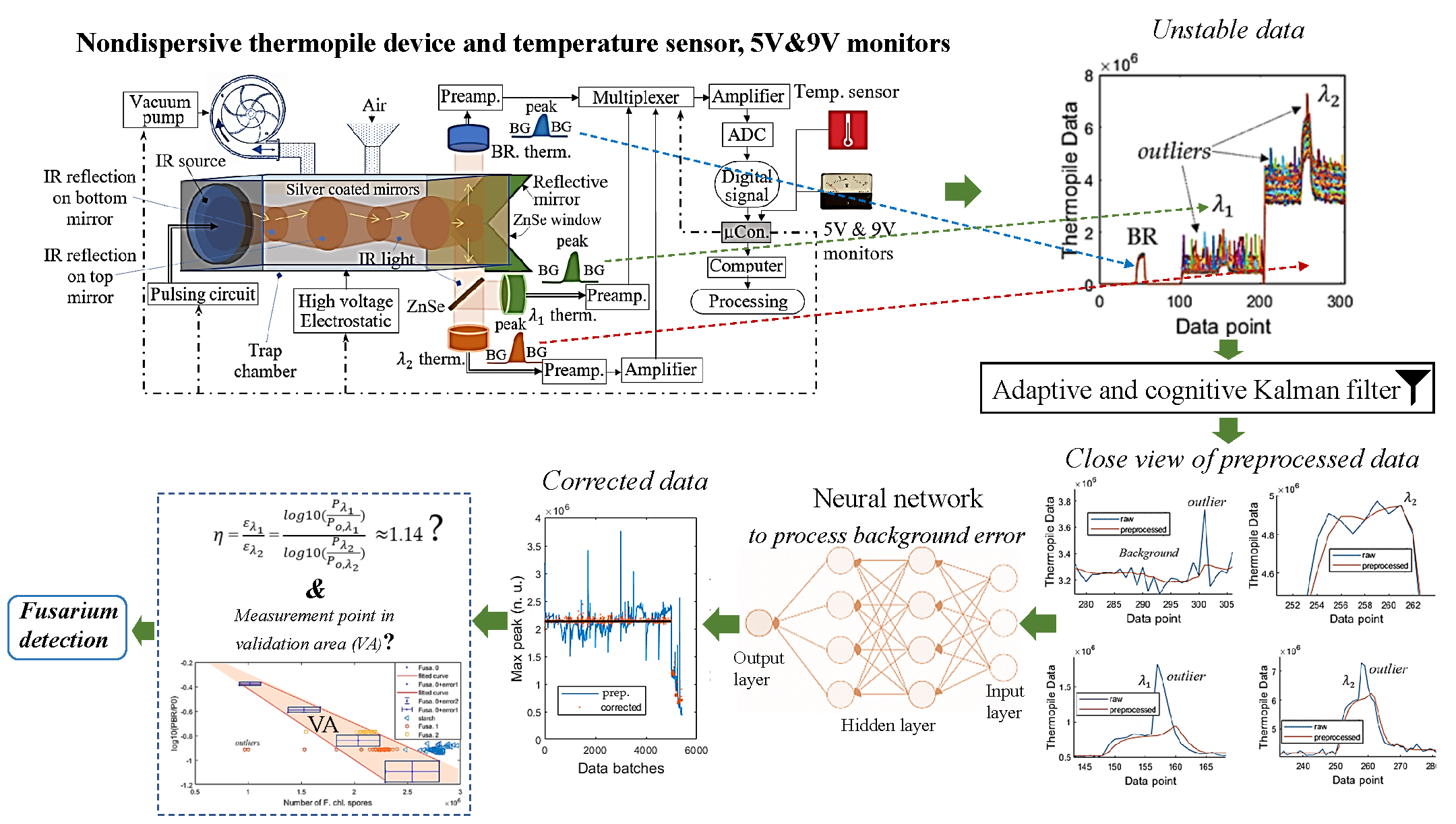
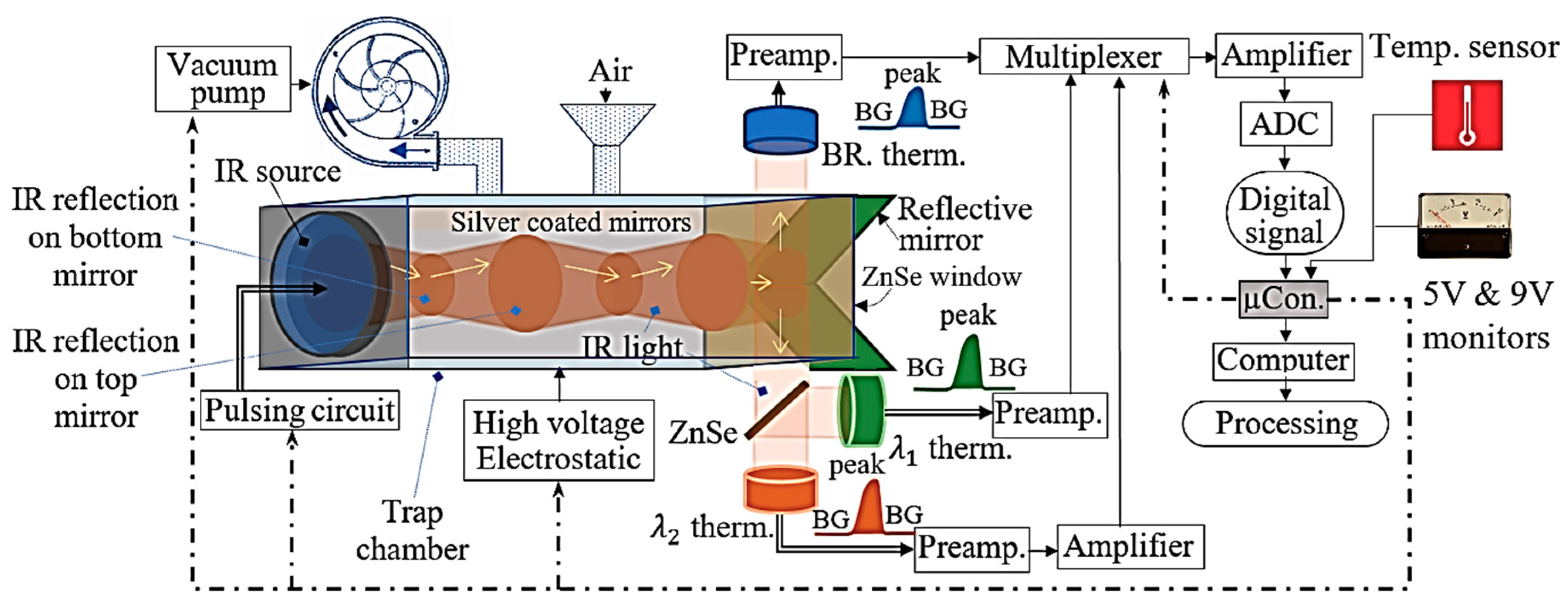
2.1. Kalman Algorithm
2.2. Neural Network
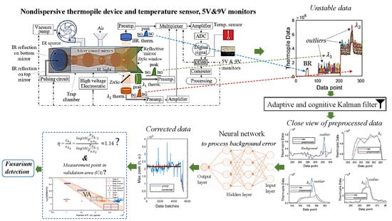
3. Methodology
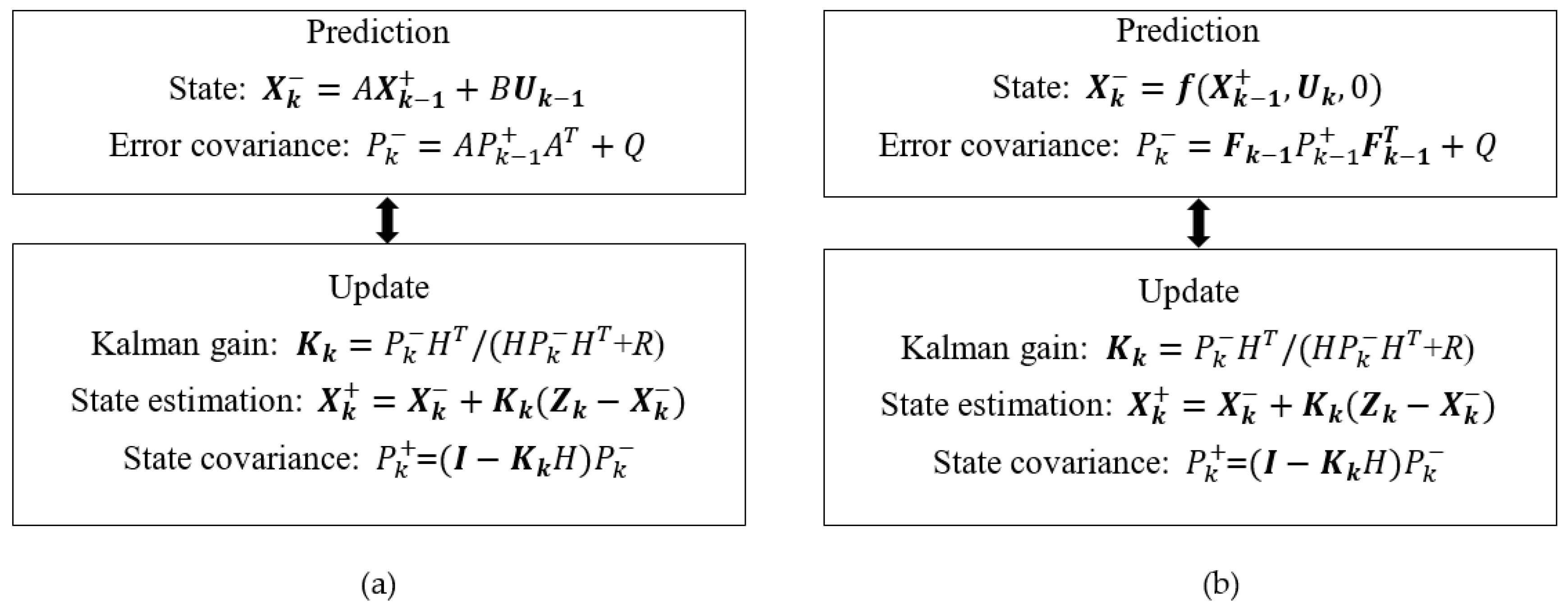
3.1. System
- Phase 1: Measuring environment temperature—T1; then, measuring outputs of the 5 V and 9 V regulators, which are V1 and V2 respectively.
- Phase 2: Measuring background data of BR thermopile in 6 s, when the IR source is still turned OFF; turning ON the IR source in 1.5 s and measuring data from the BR thermopile during this period to have peak data (PD); turning OFF the IR source in 6 s and measuring background data of the BR thermopile again. Thus, the data include background data, peak data PD and background data again.
- Phase 3: Similar to phase 2, thermopile data are measured.
- Phase 4: Similar to phase 2, thermopile data are measured.
- Phase 5: Repeating phase 1, but renaming temperature as T2, and the outputs of 5 V and 9 V regulators as V3 and V4 respectively.
- Phase 6: Sending all data to the computer in time order for further processing and analyzing.
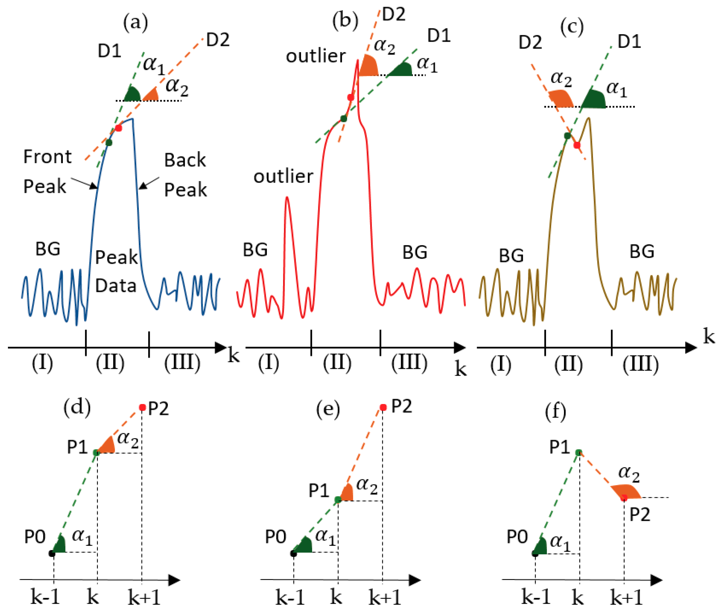
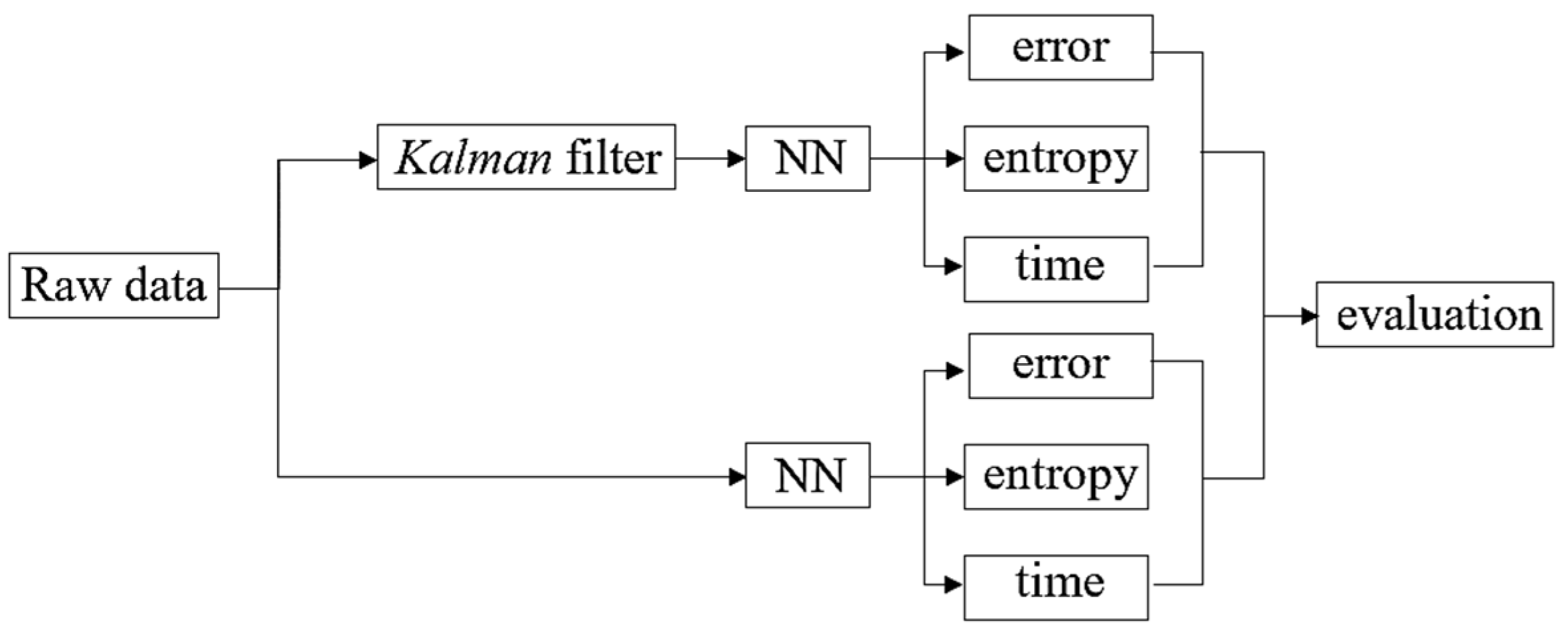
3.2. Analyzing Method
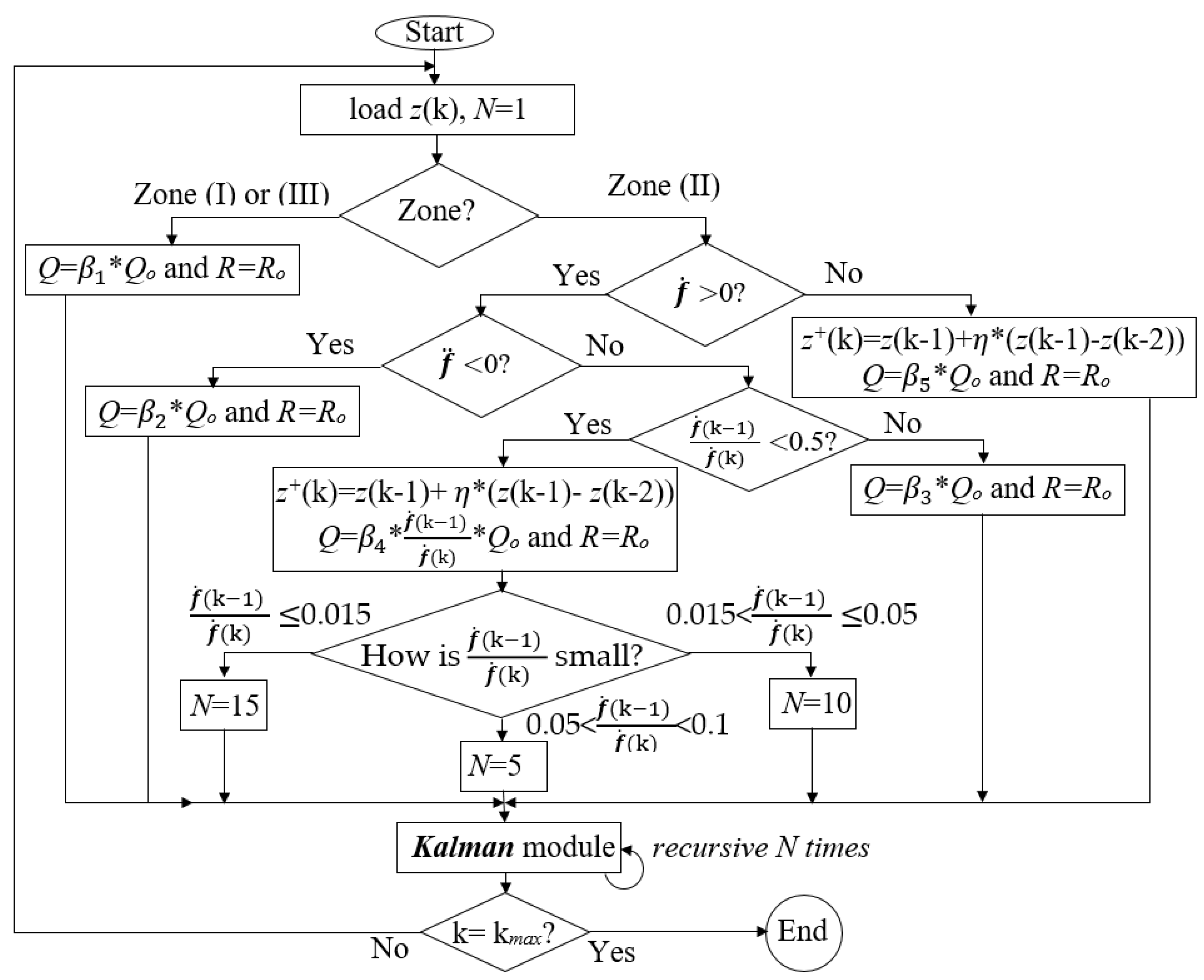
3.3. Adaptive and Cognitive Kalman Filter
3.4. Entropy
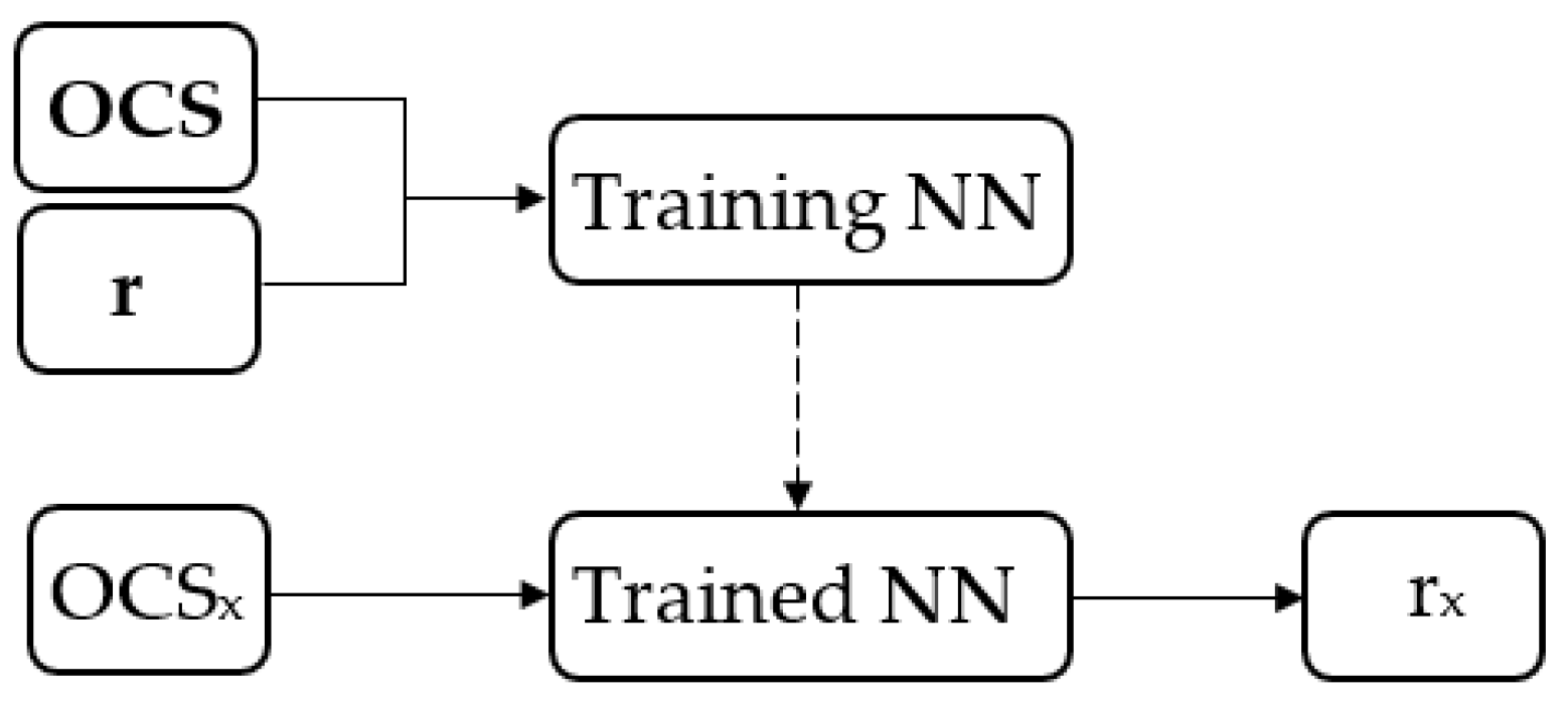
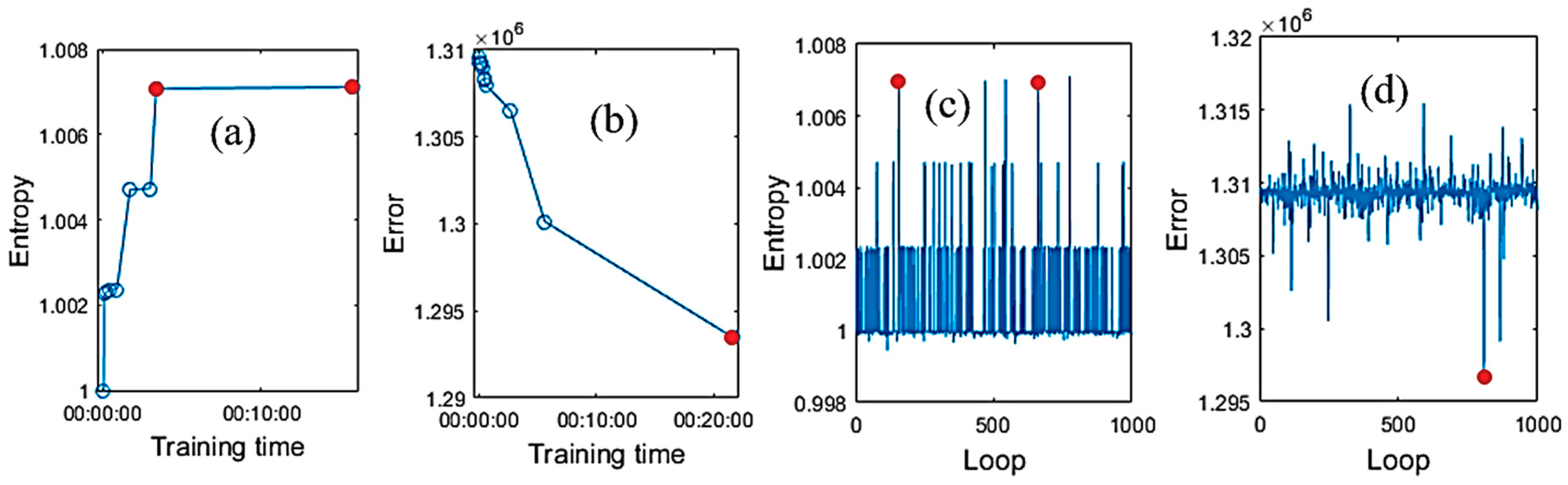
3.5. Error Correction by Neural Network
3.6. Samples
4. Results and Discussion
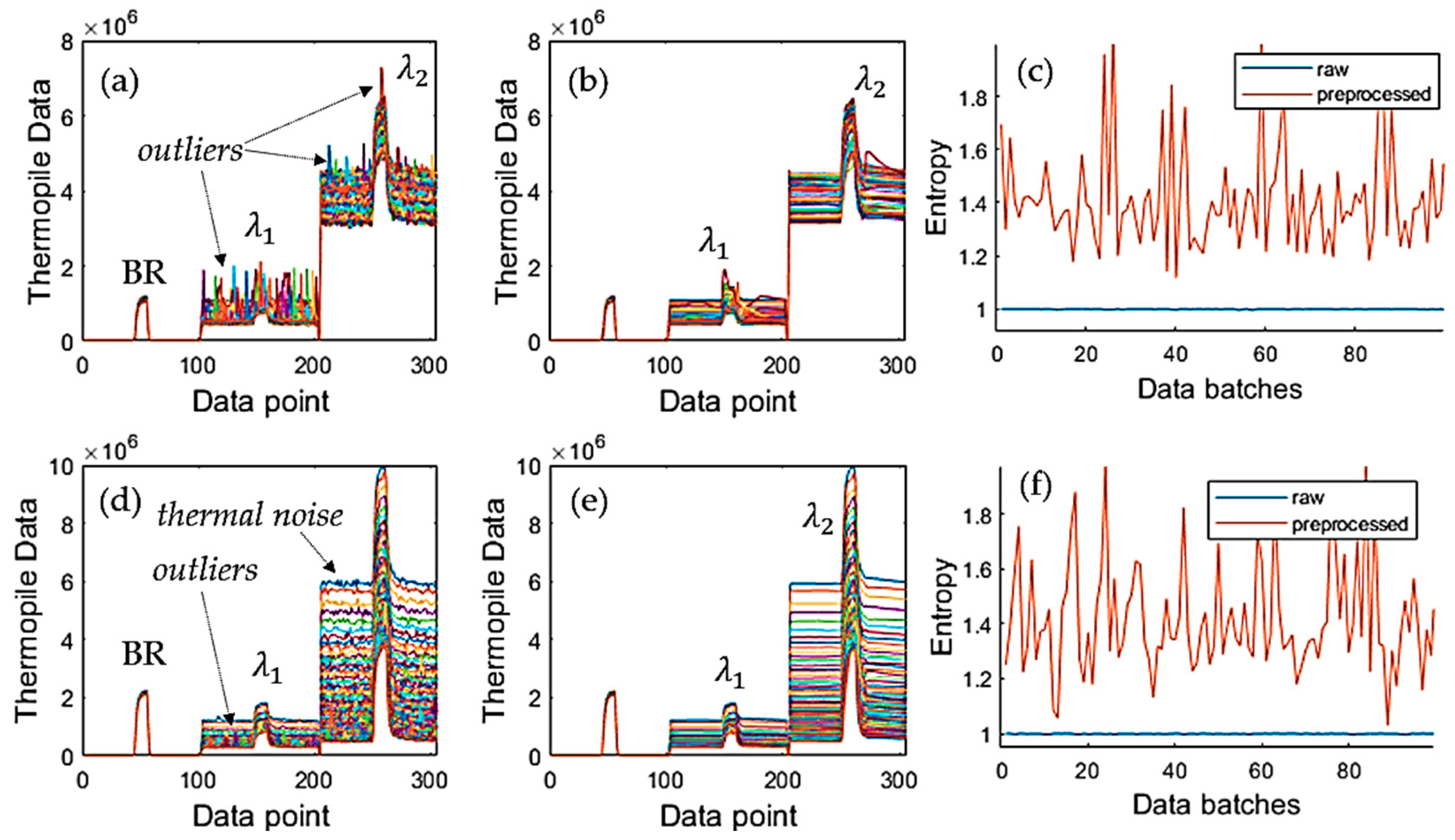
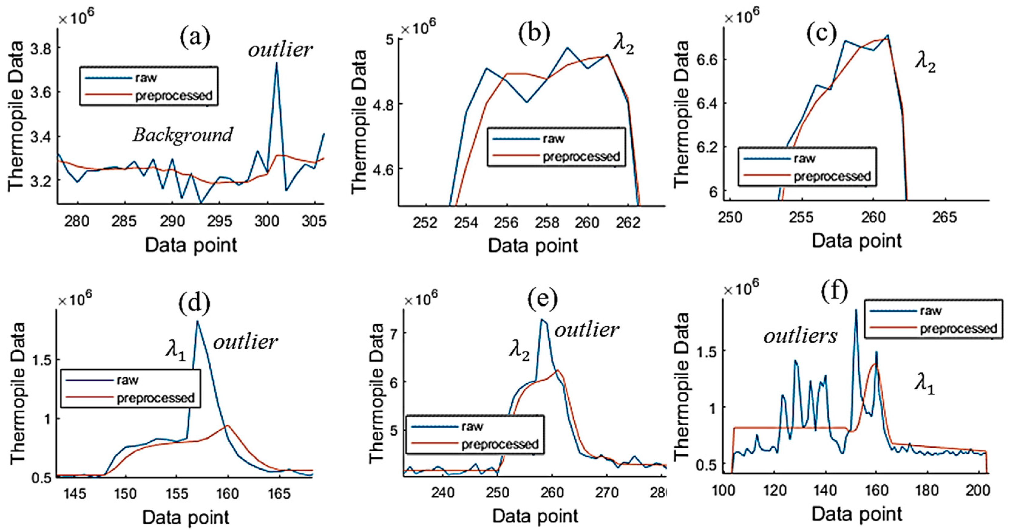
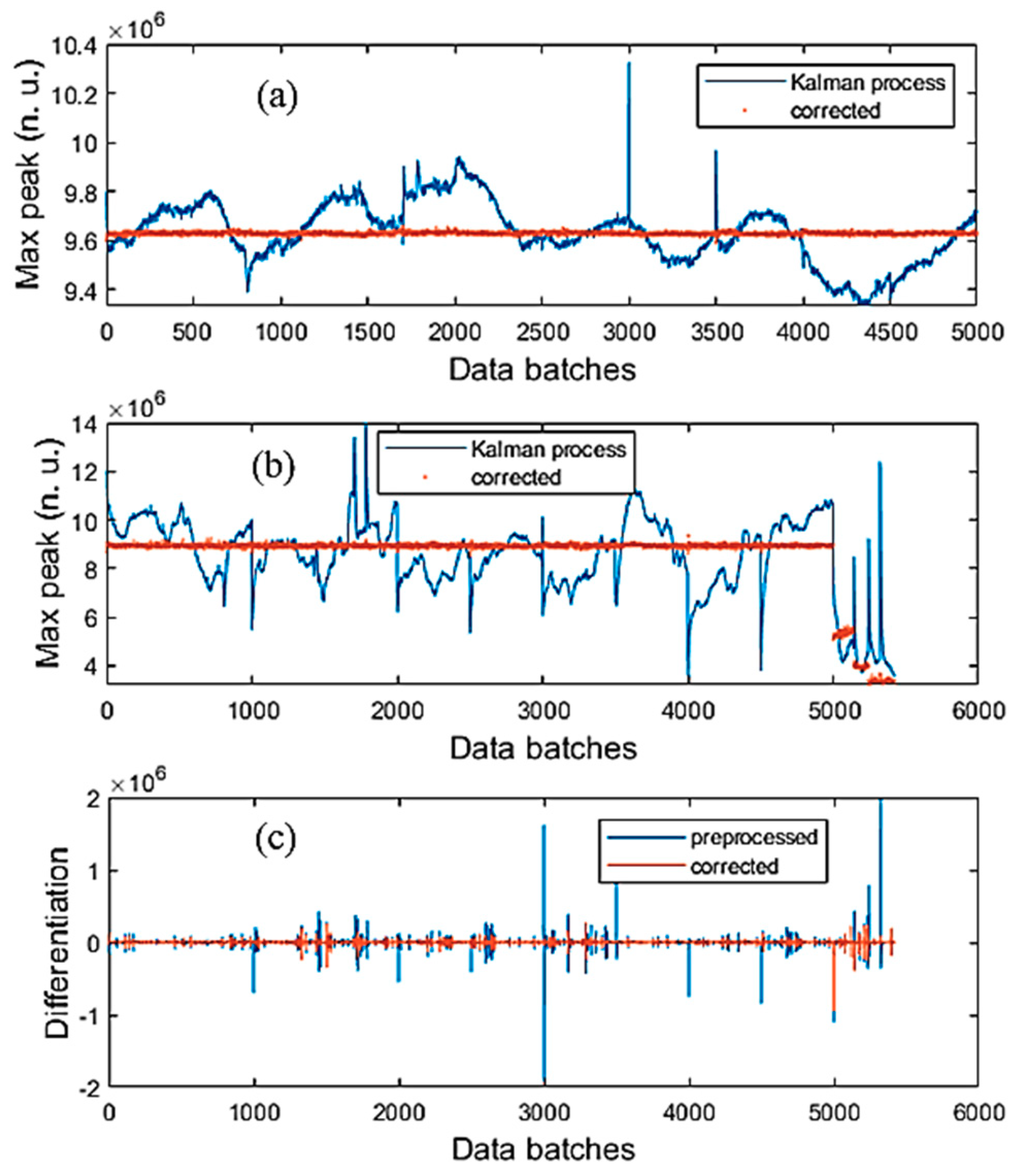
4.1. Reduction of Thermal and Burst Noises
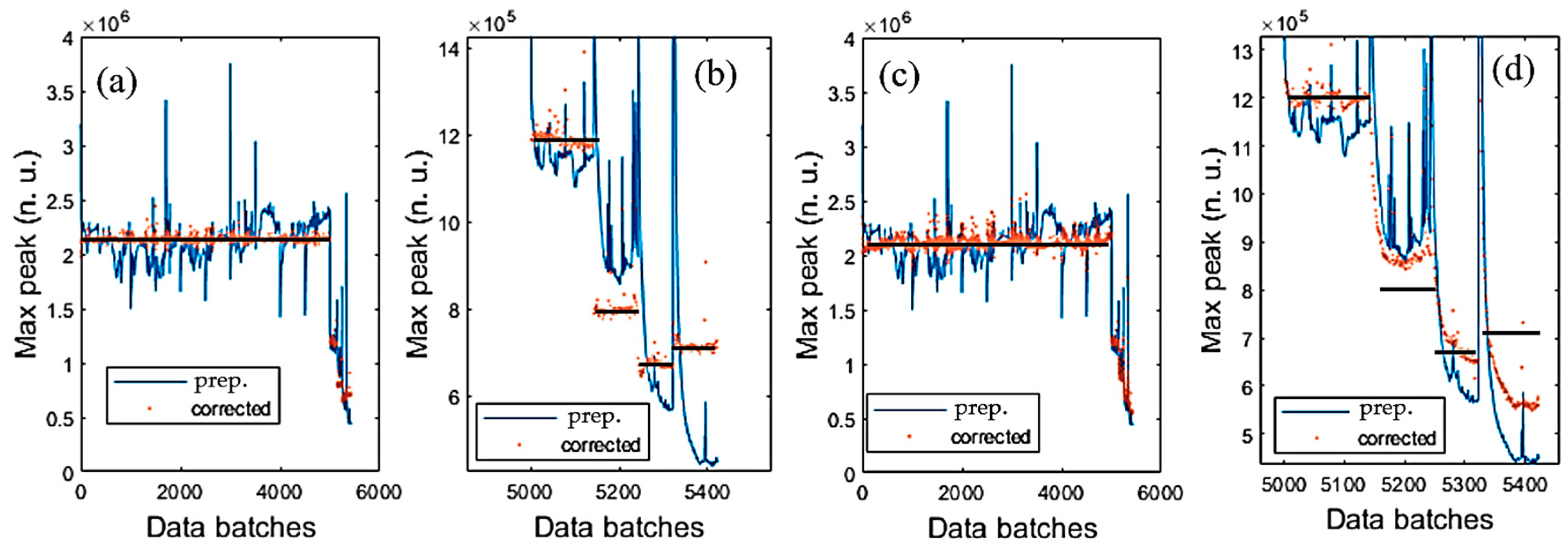
4.2. Reduction of Background Noise
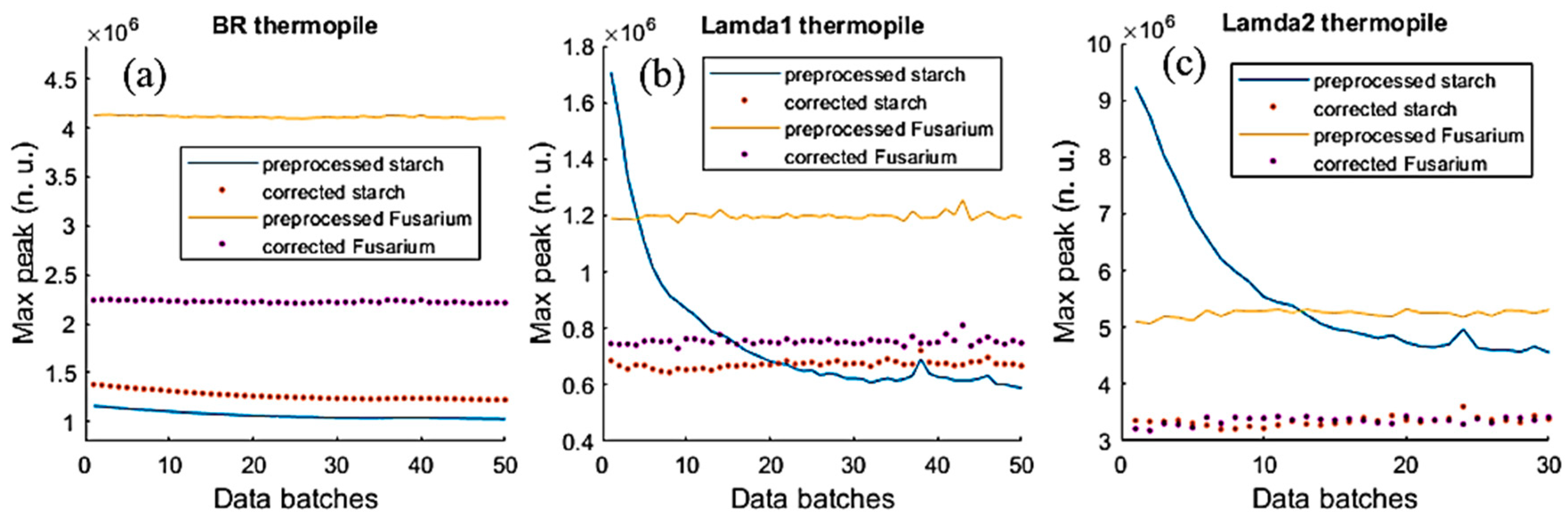
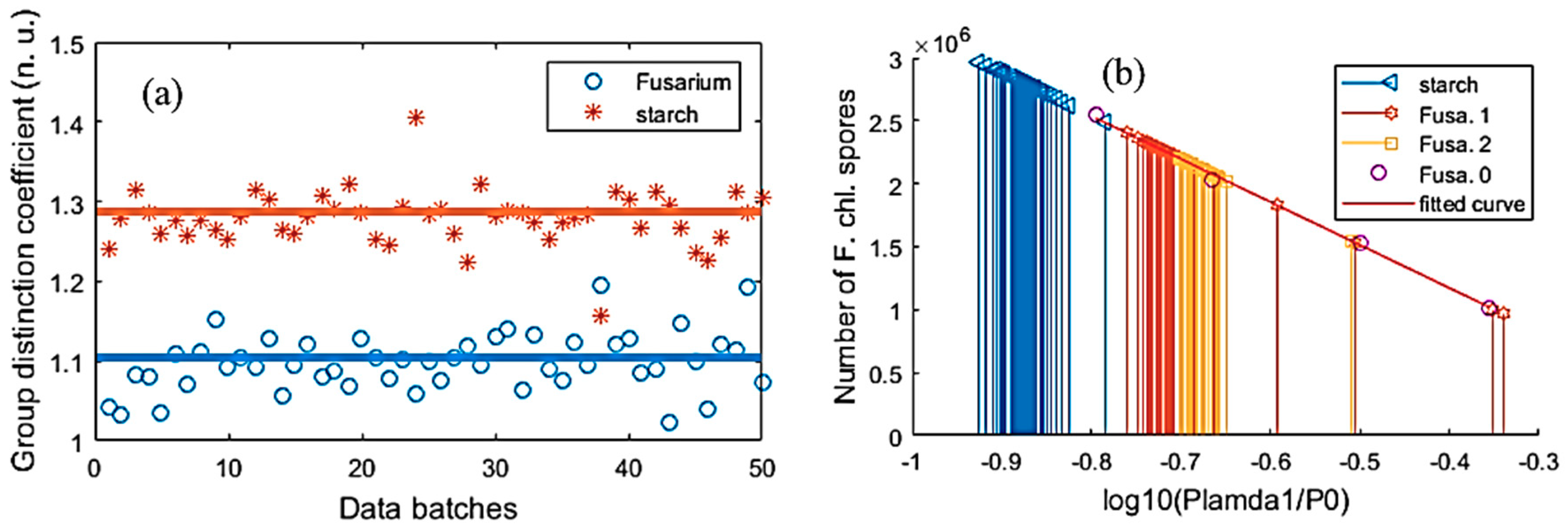
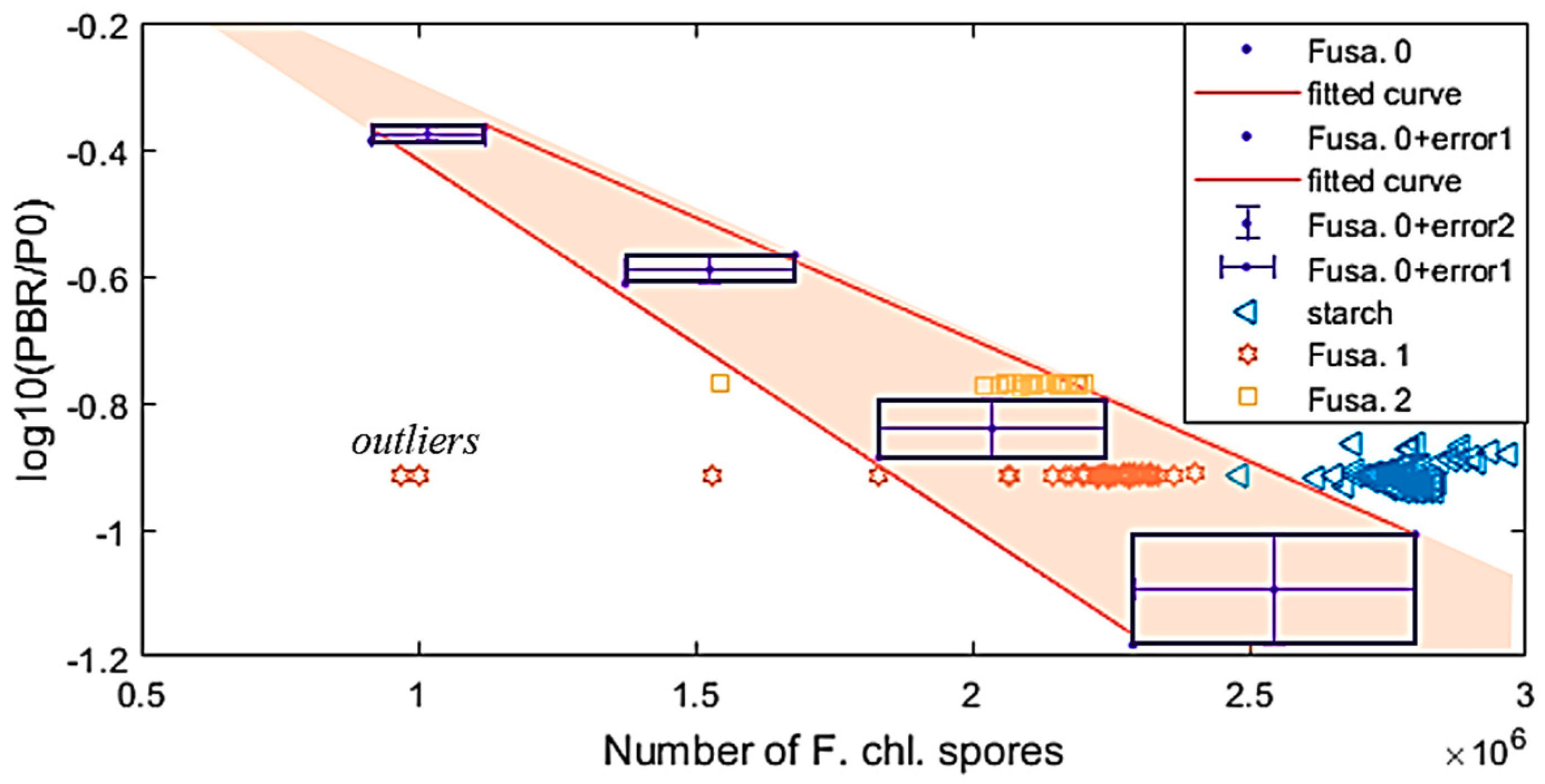
4.3. Analysis
4.4. Discussion
5. Conclusions
Author Contributions
Funding
Acknowledgments
Conflicts of Interest
References
- Nucci, M.; Anaissie, E. Fusarium Infections in Immunocompromised Patients. Clin. Microbiol. Rev. 2007, 20, 695–704. [Google Scholar] [CrossRef] [PubMed]
- Evans, J.; Levesque, D.; de Lahunta, A.; Jensen, H.E. Intracranial fusariosis: A novel cause of fungal meningoencephalitis in a dog. Vet. Pathol. 2004, 41, 510–514. [Google Scholar] [CrossRef] [PubMed]
- Martyn, R.D. Fusarium Wilt of Watermelon: 120 Years of Research. In Horticultural Reviews; Janick, J., Ed.; John Wiley & Sons, Inc.: Hoboken, NJ, USA, 2014; Volume 42, pp. 349–442. ISBN 978-1-118-91682-7. [Google Scholar]
- De Toledo-Souza, E.D.; da Silveira, P.M.; Café-Filho, A.C.; Lobo Junior, M. Fusarium wilt incidence and common bean yield according to the preceding crop and the soil tillage system. Pesq. Agropecu. Bras. 2012, 47, 1031–1037. [Google Scholar] [CrossRef]
- Bauriegel, E.; Giebel, A.; Herppich, W.B. Rapid Fusarium head blight detection on winter wheat ears using chlorophyll fluorescence imaging. J. Appl. Bot. Food Qual. 2010, 83, 196–203. [Google Scholar]
- Adesemoye, A.; Eskalen, A.; Faber, B.; Bender, G.; O’Connell, N.; Kallsen, C.; Shea, T. Current knowledge on Fusarium dry rot of citrus. Citrograph 2012, 2, 29–33. [Google Scholar]
- Foroud, N.A.; Chatterton, S.; Reid, L.M.; Turkington, T.K.; Tittlemier, S.A.; Gräfenhan, T. Fusarium Diseases of Canadian Grain Crops: Impact and Disease Management Strategies. In Future Challenges in Crop Protection against Fungal Pathogens; Goyal, A., Manoharachary, C., Eds.; Springer: New York, NY, USA, 2014; pp. 267–316. ISBN 978-1-4939-1187-5. [Google Scholar]
- BASF Canada Inc. Fusarium Management Guide; BASF Canada Inc.: Mississauga, ON, Canada, 2016; Available online: https://agro.basf.ca/basf_solutions/images/LK-CREO-B95PW8/$File/Fusarium_Management_Guide.pdf (accessed on 5 November 2019).
- Marinach-Patrice, C.; Lethuillier, A.; Marly, A.; Brossas, J.-Y.; Gené, J.; Symoens, F.; Datry, A.; Guarro, J.; Mazier, D.; Hennequin, C. Use of mass spectrometry to identify clinical Fusarium isolates. Clin. Microbiol. Infect. 2009, 15, 634–642. [Google Scholar] [CrossRef] [PubMed]
- Salman, A.; Tsror, L.; Pomerantz, A.; Moreh, R.; Mordechai, S.; Huleihel, M. FTIR spectroscopy for detection and identification of fungal phytopathogenes. Spectroscopy 2010, 24, 261–267. [Google Scholar] [CrossRef]
- Tamburini, E.; Mamolini, E.; De Bastiani, M.; Marchetti, M. Quantitative Determination of Fusarium proliferatum Concentration in Intact Garlic Cloves Using Near-Infrared Spectroscopy. Sensors 2016, 16, 1099. [Google Scholar] [CrossRef]
- West, J.S.; Canning, G.G.M.; Perryman, S.A.; King, K. Novel Technologies for the detection of Fusarium head blight disease and airborne inoculum. Trop. Plant Pathol. 2017, 42, 203–209. [Google Scholar] [CrossRef]
- Papireddy Vinayaka, P.; van den Driesche, S.; Blank, R.; Tahir, M.; Frodl, M.; Lang, W.; Vellekoop, M. An Impedance-Based Mold Sensor with on-Chip Optical Reference. Sensors 2016, 16, 1603. [Google Scholar] [CrossRef]
- Dobbs, C.G. On the primary dispersal and isolation of fungal spores. New Phytol. 1942, 41, 63–69. [Google Scholar] [CrossRef]
- Ooka, J.J.; Kommedahl, T. Wind and Rain Dispersal of Fusarium Monilifonne in Corn Fields. Available online: https://www.apsnet.org/publications/phytopathology/backissues/Documents/1977Articles/Phyto67n08_1023.PDF (accessed on 5 November 2019).
- Quesada, T.; Hughes, J.; Smith, K.; Shin, K.; James, P.; Smith, J. A Low-Cost Spore Trap Allows Collection and Real-Time PCR Quantification of Airborne Fusarium circinatum Spores. Forests 2018, 9, 586. [Google Scholar] [CrossRef]
- Lacey, J. Philip herries gregory (1907–1986). Grana 1986, 25, 159–160. [Google Scholar] [CrossRef]
- Gregory, P.H.; Guthrie, E.J.; Bunce, M.E. Experiments on Splash Dispersal of Fungus Spores. J. Gen. Microbiol. 1959, 20, 328–354. [Google Scholar] [CrossRef] [PubMed]
- Keller, M.D.; Bergstrom, G.C.; Shields, E.J. The aerobiology of Fusarium graminearum. Aerobiologia 2013, 30, 123–136. [Google Scholar] [CrossRef]
- Pham, S.; Dinh, A.; Wahid, K. A Nondispersive Thermopile Device with an Innovative Method to Detect Fusarium Spores. IEEE Sens. J. 2019, 19, 8657–8667. [Google Scholar] [CrossRef]
- Parnis, J.M.; Oldham, K.B. Oldham Journal of Photochemistry and Photobiology A: Chemistry Beyond the Beer–Lambert law: The dependence of absorbance on time in photochemistry. J. Photochem. Photobiol. A Chem. 2013, 267, 6–10. [Google Scholar] [CrossRef]
- Leslie, J.F.; Summerell, B.A. The Fusarium Laboratory Manual, 1st ed.; Blackwell Pub: Ames, IA, USA, 2006; ISBN 978-0-8138-1919-8. [Google Scholar]
- Texas Instruments Noise Analysis in Operational Amplifier Circuits. Available online: http://www.ti.com/ (accessed on 1 August 2019).
- Vasilescu, G. Physical Noise Sources. In Electronic Noise and Interfering Signals-Principles and Applications; Springer: Berlin/Heidelberg, Germany; New York, NY, USA, 2004; pp. 45–67. ISBN 3-540-40741-3. (In Germany) [Google Scholar]
- Raposo-Sánchez, M.Á.; Sáez-Landete, J.; Cruz-Roldán, F. Analog and digital filters with α-splines. Digit. Signal. Process. 2017, 66, 1–9. [Google Scholar] [CrossRef]
- Luu, L.; Dinh, A. Using Moving Average Method to Recognize Systole and Diastole on Seismocardiogram without ECG Signal. In Proceedings of the 40th Annual International Conference of the IEEE Engineering in Medicine and Biology Society (EMBC), Honolulu, HI, USA, 17–21 July 2018; pp. 3796–3799. [Google Scholar]
- Moullin, E.B.; Ellis, H.D.M. The spontaneous background noise in amplifiers due to thermal agitation and shot effects. Inst. Electr. Eng. Proc. Wirel. Sect. Inst. 1934, 9, 81–106. [Google Scholar]
- Dan, L.; Xue, W.; Guiqin, W.; Zhihong, Q. A Methodological Approach for Detecting Burst Noise in the Time Domain. Int. J. Electron. Commun. Eng. 2009, 3, 5. [Google Scholar]
- Deschrijver, D.; Knockaert, L.; Dhaene, T. Improving robustness of vector fitting to outliers in data. IEEE Electron. Lett. 2010, 46, 1200–1201. [Google Scholar] [CrossRef]
- Siouris, G.M.; Chen, G.; Wang, J. Tracking an incoming ballistic missile using an extended interval Kalman filter. IEEE Trans. Aerosp. Electron. Syst. 1997, 33, 232–240. [Google Scholar] [CrossRef]
- Zu-Tao, Z.; Jia-Shu, Z. Sampling strong tracking nonlinear unscented Kalman filter and its application in eye tracking. Chin. Phys. B 2010, 19, 104601. [Google Scholar] [CrossRef]
- Yin, S.; Na, J.H.; Choi, J.Y.; Oh, S. Hierarchical Kalman-particle filter with adaptation to motion changes for object tracking. Comput. Vis. Image Underst. 2011, 115, 885–900. [Google Scholar] [CrossRef]
- Zhang, H.; Dai, G.; Sun, J.; Zhao, Y. Unscented Kalman filter and its nonlinear application for tracking a moving target. Optik 2013, 124, 4468–4471. [Google Scholar] [CrossRef]
- Motwani, A.; Sharma, S.K.; Sutton, R.; Culverhouse, P. Interval Kalman Filtering in Navigation System Design for an Uninhabited Surface Vehicle. J. Navig. 2013, 66, 639–652. [Google Scholar] [CrossRef]
- Pham, S.; Dinh, A. Using the Kalman Algorithm to Correct Data Errors of a 24-Bit Visible Spectrometer. Sensors 2017, 17, 2939. [Google Scholar] [CrossRef]
- Lautier, D. The Kalman filter in finance: An application to term structure models of commodity prices and a comparison between the simple and the extended filters. In IDEAS Working Paper Series from RePEc; Paris Dauphine University: Paris, France, 2002. [Google Scholar]
- Bensoussan, A. Estimation and Control of Dynamical Systems; Interdisciplinary Applied Mathematics; Springer International Publishing: Cham, Switzerland, 2018; Volume 48, ISBN 978-3-319-75455-0. [Google Scholar]
- Amir, A.; Mohammadyani, D. Artificial Neural Networks: Applications in Nanotechnology; INTECH Open Access Publisher: Riịeka, Croatia, 2011; ISBN 978-953-307-188-6. [Google Scholar]
- Murphy, K.P. Machine Learning: A Probabilistic Perspective; Adaptive Computation and Machine Learning Series; MIT Press: Cambridge, MA, USA, 2012; ISBN 978-0-262-01802-9. [Google Scholar]
- Zhang, Y. Machine Learning; INTECH Open Access Publisher: Vukovar, Croatia, 2010; ISBN 978-953-307-033-9. [Google Scholar]
- Nwankpa, C.; Ijomah, W.; Gachagan, A.; Marshall, S. Activation Functions: Comparison of trends in Practice and Research for Deep Learning. Cornell Univ. 2018, 20, 1–20. [Google Scholar]
- Suzuki, K. (Ed.) Artificial Neural Networks-Architectures and Applications; InTech: Rijeka, Croatia, 2013; ISBN 978-953-51-0935-8. [Google Scholar]
- Suzuki, K. (Ed.) Artificial Neural Networks-Methodological Advances and Biomedical Applications; InTech: Rijeka, Croatia, 2011; ISBN 978-953-307-243-2. [Google Scholar]
- Amari, S.; Cichocki, A. Adaptive blind signal processing-neural network approaches. Proc. IEEE 1998, 86, 2026–2048. [Google Scholar] [CrossRef]
- Zaatri, A.; Azzizi, N.; Rahmani, F.L. Voice Recognition Technology Using Neural Networks. J. New Technol. Mater. 2015, 277, 1–5. [Google Scholar] [CrossRef]
- Huang, C.-C.; Kuo, C.-F.J.; Chen, C.-T.; Liao, C.-C.; Tang, T.-T.; Su, T.-L. Inspection of appearance defects for polarizing films by image processing and neural networks. Text. Res. J. 2016, 86, 1565–1573. [Google Scholar] [CrossRef]
- Villacorta-Atienza, J.A.; Makarov, V.A. Neural Network Architecture for Cognitive Navigation in Dynamic Environments. IEEE Trans. Neural Netw. Learn. Syst. 2013, 24, 2075–2087. [Google Scholar] [CrossRef] [PubMed]
- Northumbria Optical Narrow Band Pass. Available online: https://www.noc-ltd.com (accessed on 1 August 2019).
- 2M Thin Film Based Thermopile Detector. Available online: https://www.dexterresearch.com/ (accessed on 1 August 2019).
- Micro-Hybrid Infrared Radiation Source JSIR350-4-AL-C-D3.7-A5-I. Available online: http://www.eoc-inc.com/micro-hybrid/IRSource/JSIR350-4-AL-C-D3.7-A5-l.pdf (accessed on 1 August 2019).
- Analog Devices Zero-Drift, Single-Supply, Rail-to-Rail Input/Output Operational Amplifier AD8628/AD8629/AD8630. Available online: Analog.com (accessed on 1 August 2019).
- Texas Instruments OPAx320x Precision, 20-MHz, 0.9-pA, Low-Noise, RRIO, CMOS Operational Amplifier with Shutdown 1. Available online: http://www.ti.com (accessed on 1 August 2019).
- 24-Bit µPower No Latency ∆ΣTM ADC in SO-8. Available online: https://www.analog.com/media/en/technical-documentation/data-sheets/2400fa.pdf (accessed on 1 June 2019).
- Microchip Atmel 8-Bit Microcontroller with 4/8/16/32kbytes In-System Programmable Flash. Available online: https://www.microchip.com (accessed on 1 August 2019).
- Sabirov, D.S. Information entropy changes in chemical reactions. Comput. Theor. Chem. 2018, 1123, 169–179. [Google Scholar] [CrossRef]
- Shannon, C.E. A Mathematical Theory of Communication. Sigmob. Mob. Comput. Commun. Rev. 2001, 5, 3–55. [Google Scholar] [CrossRef]
- Aydın, S.; Saraoğlu, H.M.; Kara, S. Log Energy Entropy-Based EEG Classification with Multilayer Neural Networks in Seizure. Ann. Biomed. Eng. 2009, 37, 2626–2630. [Google Scholar] [CrossRef]


| Illustration | Thermopile | Entropies of Diff. of Raw Signal | Entropies of Diff. of Preprocessed Signal | |
|---|---|---|---|---|
 | BR | 1,162,693 | 0.9964 | 1.2808 |
| 9471 | 0.9993 | 0.9964 | ||
| 1873 | 0.9964 | 2.2958 |
| Raw data | Prep. Data | Raw Data | Prep. Data | |
|---|---|---|---|---|
| Time | 12 min 09 s | 00 min 46 s | 9 min 13 s | 1 min 00 s |
| Error | 2.7453 × 10⁴ | 1.4374 × 10⁴ | 2.3999 × 10⁵ | 1.76485 × 10⁵ |
| Entropy Operating Criterion | Error Operating Criterion | |
|---|---|---|
| Time | 15 min 47 s | 21 min 37 s |
| Optimal entropy | 1.0071 | N/A |
| Optimal Error | N/A | 1,293,496.24 |
| Entropy | N/A | 0.9999 |
| Error | 1.2935 × 10⁶ | N/A |
| Fusarium | Starch | |
|---|---|---|
| η | 1.125 | 1.31 |
| 0.110 | 0.06 | |
| 9.8% | 4.6% |
© 2019 by the authors. Licensee MDPI, Basel, Switzerland. This article is an open access article distributed under the terms and conditions of the Creative Commons Attribution (CC BY) license (http://creativecommons.org/licenses/by/4.0/).
Share and Cite
Pham, S.; Dinh, A. Adaptive-Cognitive Kalman Filter and Neural Network for an Upgraded Nondispersive Thermopile Device to Detect and Analyze Fusarium Spores. Sensors 2019, 19, 4900. https://doi.org/10.3390/s19224900
Pham S, Dinh A. Adaptive-Cognitive Kalman Filter and Neural Network for an Upgraded Nondispersive Thermopile Device to Detect and Analyze Fusarium Spores. Sensors. 2019; 19(22):4900. https://doi.org/10.3390/s19224900
Chicago/Turabian StylePham, Son, and Anh Dinh. 2019. "Adaptive-Cognitive Kalman Filter and Neural Network for an Upgraded Nondispersive Thermopile Device to Detect and Analyze Fusarium Spores" Sensors 19, no. 22: 4900. https://doi.org/10.3390/s19224900
APA StylePham, S., & Dinh, A. (2019). Adaptive-Cognitive Kalman Filter and Neural Network for an Upgraded Nondispersive Thermopile Device to Detect and Analyze Fusarium Spores. Sensors, 19(22), 4900. https://doi.org/10.3390/s19224900