Surface Deformation Analysis of the Wider Zagreb Area (Croatia) with Focus on the Kašina Fault, Investigated with Small Baseline InSAR Observations


Abstract
1. Introduction
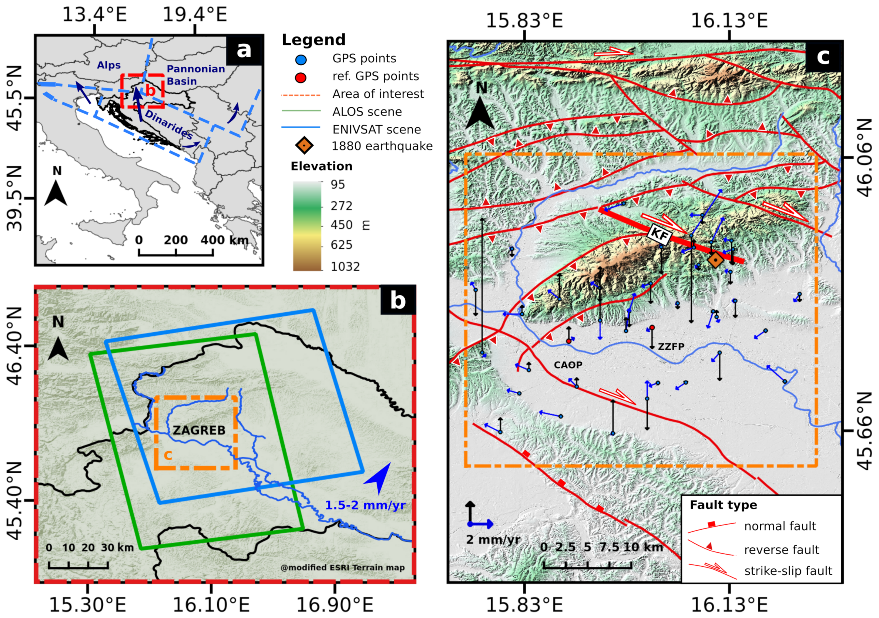
2. Study Area
3. Small Baseline Interferometry
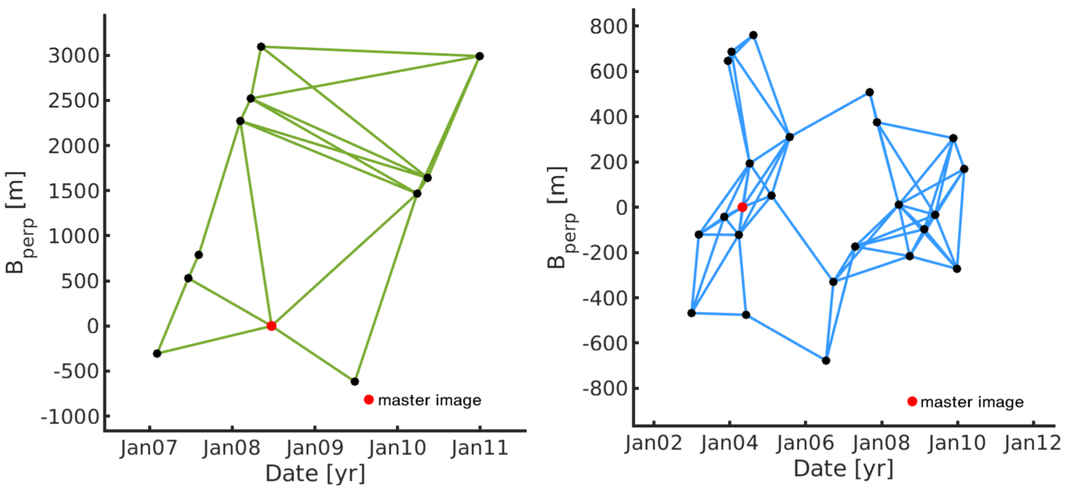
3.1. Data
3.2. Data Processing and Post-Processing
4. Results
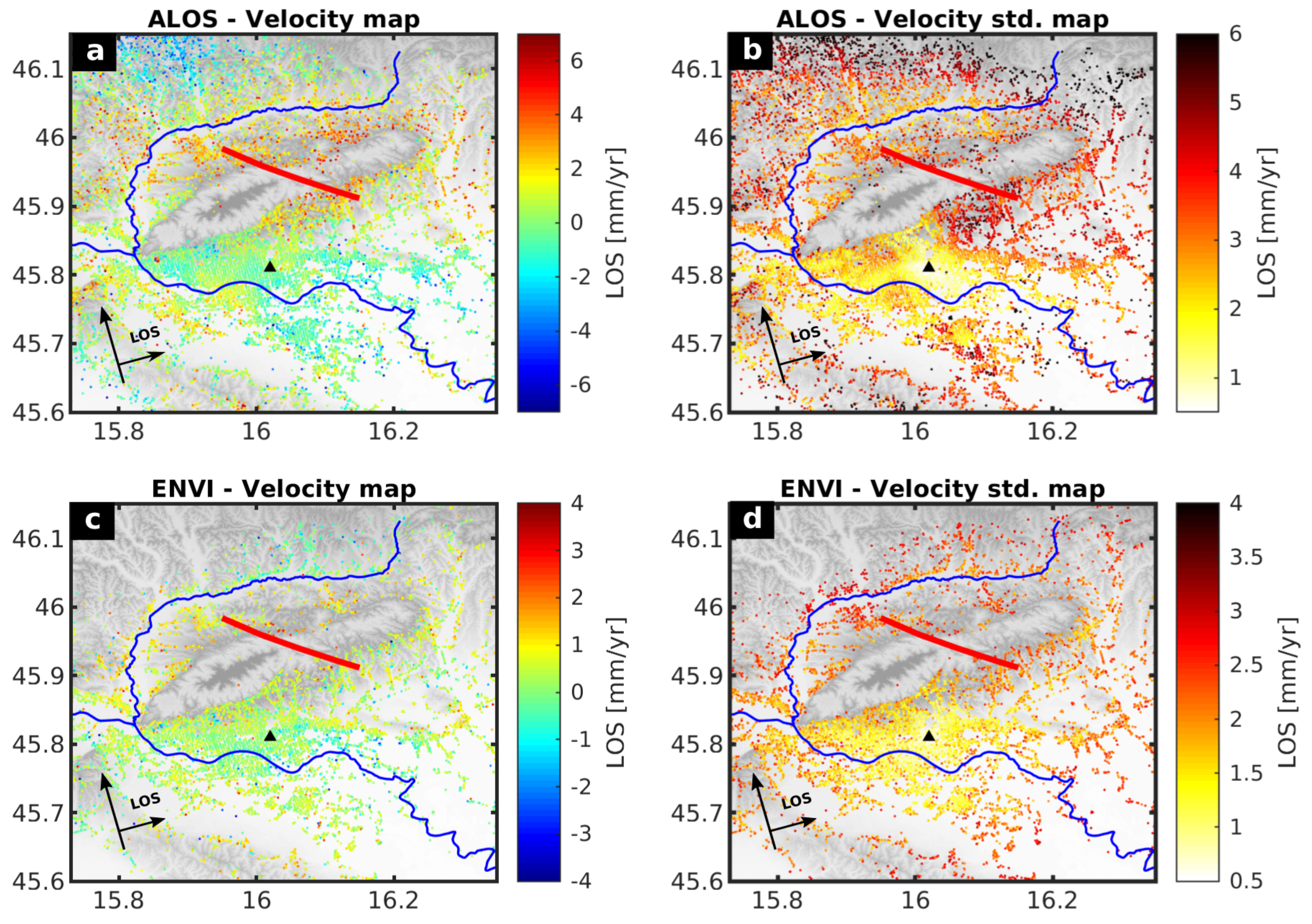
4.1. Small Baseline Interferometry Velocity Fields
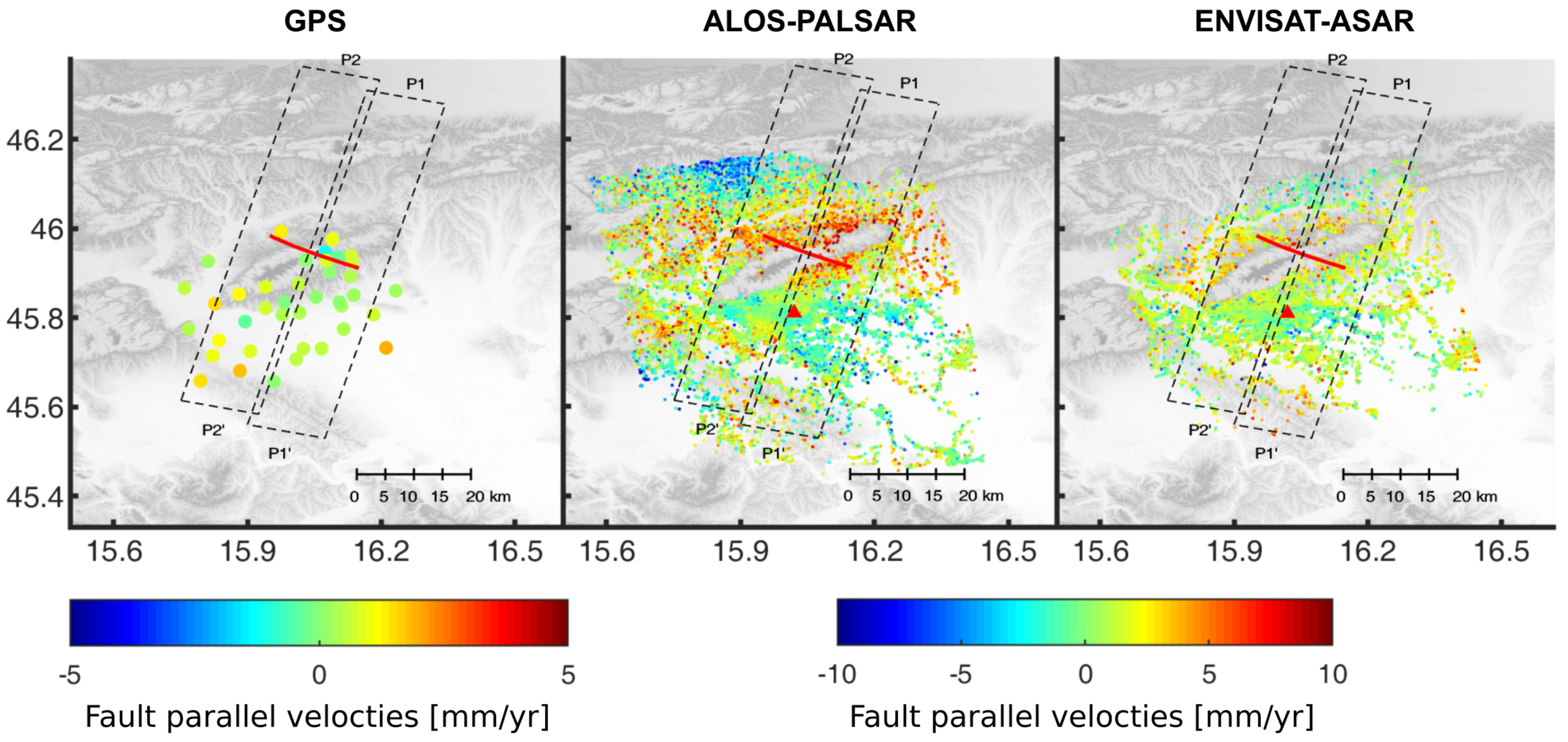
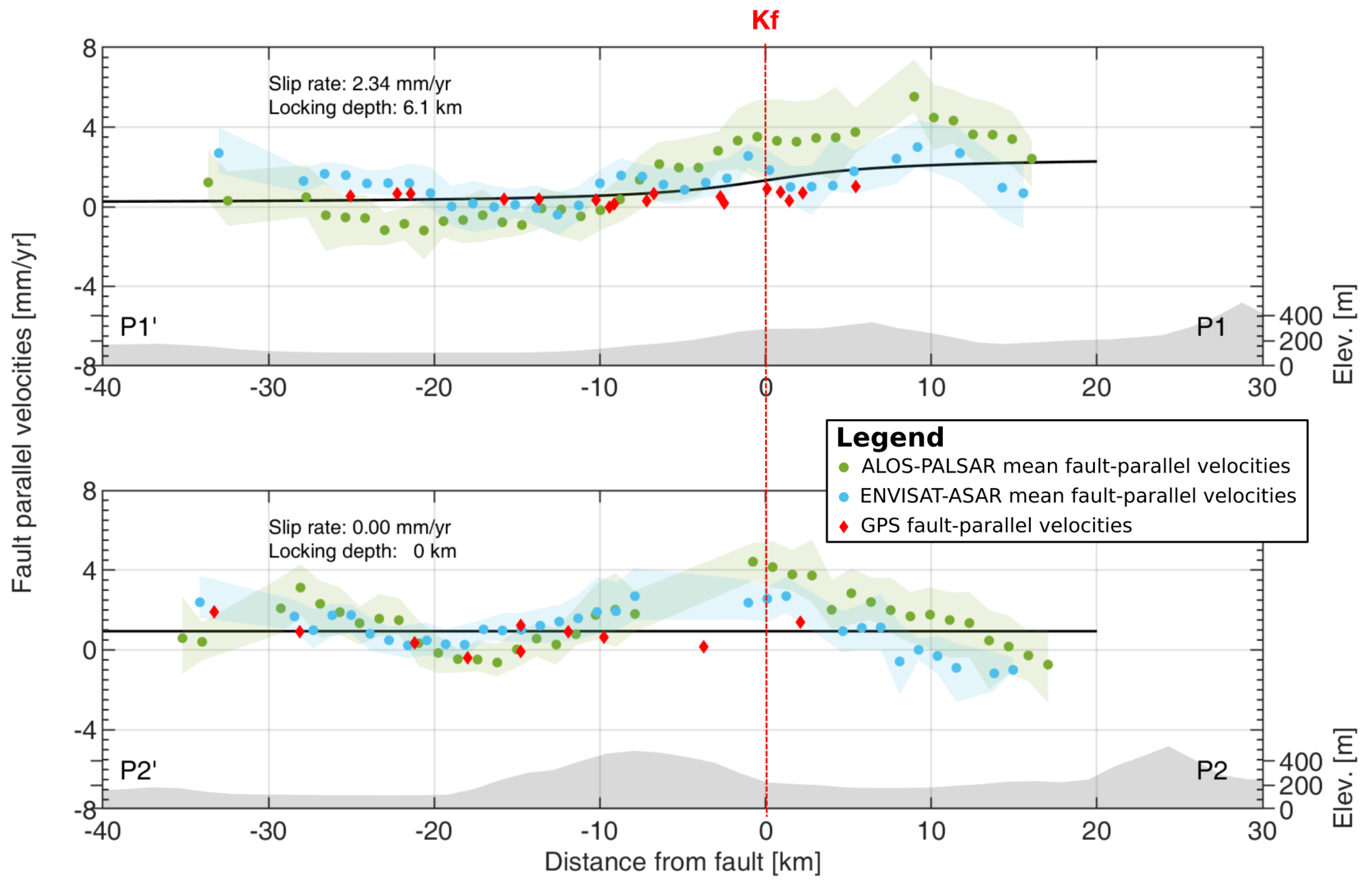
4.2. Interseismic Strain Accumulation Analysis on the Kašina Fault
5. Discussion
6. Conclusions
Author Contributions
Funding
Acknowledgments
Conflicts of Interest
References
- Prelogović, E.; Saftić, B.; Kuk, V.; Velić, J.; Dragaš, M.; Lučić, D. Tectonic activity in the Croatian part of the Pannonian basin. Tectonophysics 1998, 297, 283–293. [Google Scholar] [CrossRef]
- Herak, D.; Herak, M.; Tomljenović, B. Seismicity and earthquake focal mechanisms in North-Western Croatia. Tectonophysics 2009, 465, 212–220. [Google Scholar] [CrossRef]
- Markušić, S.; Herak, M. Seismic zoning of Croatia. Nat. Hazards 1999, 18, 269–285. [Google Scholar] [CrossRef]
- Tomljenović, B.; Csontos, L. Neogene-quaternary structures in the border zone between Alps, Dinarides and Pannonian Basin (Hrvatsko zagorje and Karlovac Basins, Croatia). Int. J. Earth Sci. 2001, 90, 560–578. [Google Scholar] [CrossRef]
- Grenerczy, G.; Sella, G.; Stein, S.; Kenyeres, A. Tectonic implications of the GPS velocity field in the northern Adriatic region. Geophys. Res. Lett. 2005, 32, l16311. [Google Scholar] [CrossRef]
- Grenerczy, G.; Kenyeres, A.; Fejes, I. Present crustal movement and strain distribution in Central Europe inferred from GPS measurements. J. Geophys. Res. Solid Earth 2000, 105, 21835–21846. [Google Scholar] [CrossRef]
- Matoš, B.; Tomljenović, B.; Trenc, N. Identification of tectonically active areas using DEM: a quantitative morphometric analysis of Mt. Medvednica, NW Croatia. Geol. Q. 2014, 58, 51–70. [Google Scholar] [CrossRef][Green Version]
- Pribičević, B.; Medak, D.; Đapo, A. Geodetic contribution to the geodynamic research of the area of the City of Zagreb. In Annual 2010/2011 of the Croatian Academy of Engineering; Croatian Academy of Engineering: Zagreb, Croatia, 2012; pp. 11–22. [Google Scholar]
- Pribičević, B.; Đapo, A. Movement analysis on Geodynamic network of the City of Zagreb from different time epochs. Geod. List 2016, 70, 207–230. [Google Scholar]
- Pribičević, B.; Đapo, A.; Govorčin, M. The application of satellite technology in the study of geodynamic movements in the wider Zagreb area. Tehnički Vjesnik 2017, 24, 503–512. [Google Scholar]
- Berardino, P.; Fornaro, G.; Lanari, R.; Sansosti, E. A new algorithm for surface deformation monitoring based on small baseline differential SAR interferograms. IEEE Trans. Geosci. Remote Sens. 2002, 40, 2375–2383. [Google Scholar] [CrossRef]
- Bekaert, D.; Walters, R.; Wright, T.; Hooper, A.; Parker, D. Statistical comparison of InSAR tropospheric correction techniques. Remote Sens. Environ. 2015, 170, 40–47. [Google Scholar] [CrossRef]
- Herak, D.; Cabor, S. Earthquake catalogue for SR Croatia (Yugoslavia) and neighbouring regions for the years 1986 and 1987. Geofizika 1989, 6, 101–121. [Google Scholar]
- Markušić, S.; Herak, D.; Ivančić, I.; Sović, I.; Herak, M.; Prelogović, E. Seismicity of Croatia in the period 1993–1996 and the Ston-Slano earthquake of 1996. Geofizika 1998, 15, 83–101. [Google Scholar]
- Ivančić, I.; Herak, D.; Markušić, S.; Sović, I.; Herak, M. Seismicity of Croatia in the period 1997–2001/Seizmicnost Hrvatske u razdoblju 1997–2001. Geofizika 2002, 18, 17–29. [Google Scholar]
- Ivančić, I.; Herak, D.; Markušić, S.; Sović, I.; Herak, M. Seismicity of Croatia in the period 2002–2005. Geofizika 2006, 23, 87–104. [Google Scholar]
- Ivančić, I.; Herak, D.; Herak, M.; Allegretti, I.; Fiket, T.; Kuk, K.; Markušić, S.; Prevolnik, S.; Sović, I.; Dasović, I.; et al. Seismicity of Croatia in the period 2006–2015. Geofizika 2018, 35, 69–98. [Google Scholar] [CrossRef]
- Ferretti, A.; Prati, C.; Rocca, F. Permanent scatterers in SAR interferometry. IEEE Trans. Geosci. Remote Sens. 2001, 39, 8–20. [Google Scholar] [CrossRef]
- Lanari, R.; Mora, O.; Manunta, M.; Mallorquí, J.J.; Berardino, P.; Sansosti, E. A small-baseline approach for investigating deformations on full-resolution differential SAR interferograms. IEEE Trans. Geosci. Remote Sens. 2004, 42, 1377–1386. [Google Scholar] [CrossRef]
- Hooper, A. A multi-temporal InSAR method incorporating both persistent scatterer and small baseline approaches. Geophys. Res. Lett. 2008, 35. [Google Scholar] [CrossRef]
- Hetland, E.; Musé, P.; Simons, M.; Lin, Y.; Agram, P.; DiCaprio, C. Multiscale InSAR time series (MInTS) analysis of surface deformation. J. Geophys. Res. Solid Earth 2012, 117. [Google Scholar] [CrossRef]
- Gong, W.; Thiele, A.; Hinz, S.; Meyer, F.J.; Hooper, A.; Agram, P.S. Comparison of Small Baseline Interferometric SAR Processors for Estimating Ground Deformation. Remote Sens. 2016, 8, 330. [Google Scholar] [CrossRef]
- Hooper, A.; Bekaert, D.; Spaans, K.; Arıkan, M. Recent advances in SAR interferometry time series analysis for measuring crustal deformation. Tectonophysics 2012, 514, 1–13. [Google Scholar] [CrossRef]
- Sandwell, D.T.; Myer, D.; Mellors, R.; Shimada, M.; Brooks, B.; Foster, J. Accuracy and resolution of ALOS interferometry: Vector deformation maps of the Father’s Day intrusion at Kilauea. IEEE Trans. Geosci. Remote Sens. 2008, 46, 3524–3534. [Google Scholar] [CrossRef]
- ECMWF. ERA5 Reanalysis Datasets. Available online: https://www.ecmwf.int/en/forecasts/datasets/reanalysis-datasets/era5 (accessed on 20 July 2019).
- Pribičević, B.; Đapo, A.; Prelogović, E. The combined space-time analysis of geodetic and geological surveys on the geodynamic network of the wider Zagreb area. 2019; in preparation. [Google Scholar]
- Herring, T.; King, R.; McClusky, S. Introduction to GAMIT/GLOBK; Release 10.6; Massachusetts Institute of Technology: Cambridge, MA, USA, 2015. [Google Scholar]
- Doornbos, E.; Scharroo, R.; Klinkrad, H.; Zandbergen, R.; Fritsche, B. Improved modelling of surface forces in the orbit determination of ERS and Envisat. Can. J. Remote Sens. 2002, 28, 535–543. [Google Scholar] [CrossRef]
- Hanssen, R.F. Radar Interferometry: Data Interpretation and Error Analysis; Springer Science & Business Media: Berlin/Heidelberg, Germany, 2001. [Google Scholar]
- Kampes, B.M.; Hanssen, R.F.; Perski, Z. Radar interferometry with public domain tools. In Proceedings of the FRINGE, Frascati, Italy, 1–5 December 2003; Volume 3. [Google Scholar]
- Hooper, A.; Zebker, H.; Segall, P.; Kampes, B. A new method for measuring deformation on volcanoes and other natural terrains using InSAR persistent scatterers. Geophys. Res. Lett. 2004, 31. [Google Scholar] [CrossRef]
- Hooper, A.; Segall, P.; Zebker, H. Persistent scatterer interferometric synthetic aperture radar for crustal deformation analysis, with application to Volcán Alcedo, Galápagos. J. Geophys. Res. Solid Earth 2007, 112. [Google Scholar] [CrossRef]
- Marinkovic, P.; Ketelaar, G.; van Leijen, F.; Hanssen, R. InSAR quality control: Analysis of five years of corner reflector time series. In Proceedings of the Fringe 2007 Workshop (ESA SP-649), Frascati, Italy, 26–30 November 2007; Volume 26, p. 30. [Google Scholar]
- Tomljenović, B.; Csontos, L.; Márton, E.; Márton, P. Tectonic evolution of the northwestern Internal Dinarides as constrained by structures and rotation of Medvednica Mountains, North Croatia. Geol. Soc. Lond. Spec. Publ. 2008, 298, 145–167. [Google Scholar] [CrossRef]
- Savage, J.; Burford, R. Geodetic determination of relative plate motion in central California. J. Geophys. Res. 1973, 78, 832–845. [Google Scholar] [CrossRef]
- Kuk, V.; Prelogović, E.; Sović, I.; Kuk, K.; Šariri, K. Seismological and seismo-tectonical properties of the wider Zagreb area. Građevinar 2000, 52, 647–653. [Google Scholar]
- Fattahi, H.; Amelung, F. InSAR uncertainty due to orbital errors. Geophys. J. Int. 2014, 199, 549–560. [Google Scholar] [CrossRef]


| Satellite Mission | ALOS-PALSAR | Envisat-ASAR | |
|---|---|---|---|
| Wavelength [cm] | 23.6 | 5.6 | |
| First date (yyyy-mm-dd) | 2007-02-03 | 2002-12-28 | |
| Last date (yyyy-mm-dd) | 2010-12-30 | 2010-07-24 | |
| Orbit direction | Ascending | Ascending | |
| Inc. angle [deg] | 38.75 | 21.1 | |
| Acquist. mode | Fine Single Beam | Fine Dual Beam | Stripmap |
| Imaging mode | HH or VV | HH + HV or VV + VH | HH or VV |
| Spatial resolution (range × azimuth [m] ) | 4.68 × 3.13 | 9.37 × 3.14 | 7.81 × 4.04 |
| Critc. perp. baseline [km] | 13.1 | 6.5 | 1.1 |
| Numb. of images | 6 | 8 | 27 |
| StaMPS-SB Parameters | ALOS-PALSAR | Envisat-ASAR |
|---|---|---|
| Number of interferograms | 21 | 64 |
| Weed standard deviation | 0.6 | 0.8 |
| Weed time window [days] | 1100 | 1100 |
| Merge resample size | 300 | 300 |
| Merge standard deviation | 0.2 | 0.4 |
| Unwrap grid size [m] | 100 | 100 |
| Unwrap time [days] | 1500 | 1500 |
| Reference point [Lon Lat] [deg] | 16.02 45.81 | 16.02 45.81 |
| Reference radius | 500 | 500 |
| Statistics | ALOS-PALSAR | Envisat-ASAR | |||
|---|---|---|---|---|---|
| Before Filtering | After Filtering | Before Filtering | After Filtering | ||
| Num. of DS points [#] | 15,033 | 12,430 | 8922 | 8094 | |
| Velocity model [mm/year] | Median | 0.51 | 0.52 | 0.40 | 0.41 |
| Interquartile range | 2.01 | 1.99 | 0.77 | 0.75 | |
| Stand. dev. model [mm/year] | Median | 3.49 | 3.12 | 2.00 | 1.93 |
| Interquartile range | 2.56 | 1.72 | 0.77 | 0.75 | |
© 2019 by the authors. Licensee MDPI, Basel, Switzerland. This article is an open access article distributed under the terms and conditions of the Creative Commons Attribution (CC BY) license (http://creativecommons.org/licenses/by/4.0/).
Share and Cite
Govorčin, M.; Pribičević, B.; Wdowinski, S. Surface Deformation Analysis of the Wider Zagreb Area (Croatia) with Focus on the Kašina Fault, Investigated with Small Baseline InSAR Observations. Sensors 2019, 19, 4857. https://doi.org/10.3390/s19224857
Govorčin M, Pribičević B, Wdowinski S. Surface Deformation Analysis of the Wider Zagreb Area (Croatia) with Focus on the Kašina Fault, Investigated with Small Baseline InSAR Observations. Sensors. 2019; 19(22):4857. https://doi.org/10.3390/s19224857
Chicago/Turabian StyleGovorčin, Marin, Boško Pribičević, and Shimon Wdowinski. 2019. "Surface Deformation Analysis of the Wider Zagreb Area (Croatia) with Focus on the Kašina Fault, Investigated with Small Baseline InSAR Observations" Sensors 19, no. 22: 4857. https://doi.org/10.3390/s19224857
APA StyleGovorčin, M., Pribičević, B., & Wdowinski, S. (2019). Surface Deformation Analysis of the Wider Zagreb Area (Croatia) with Focus on the Kašina Fault, Investigated with Small Baseline InSAR Observations. Sensors, 19(22), 4857. https://doi.org/10.3390/s19224857