The Influence of Temperature and Community Structure on Light Absorption by Phytoplankton in the North Atlantic

 ,
, 
 , and
, and 
Abstract

1. Introduction
2. Methodology
2.1. Study Area
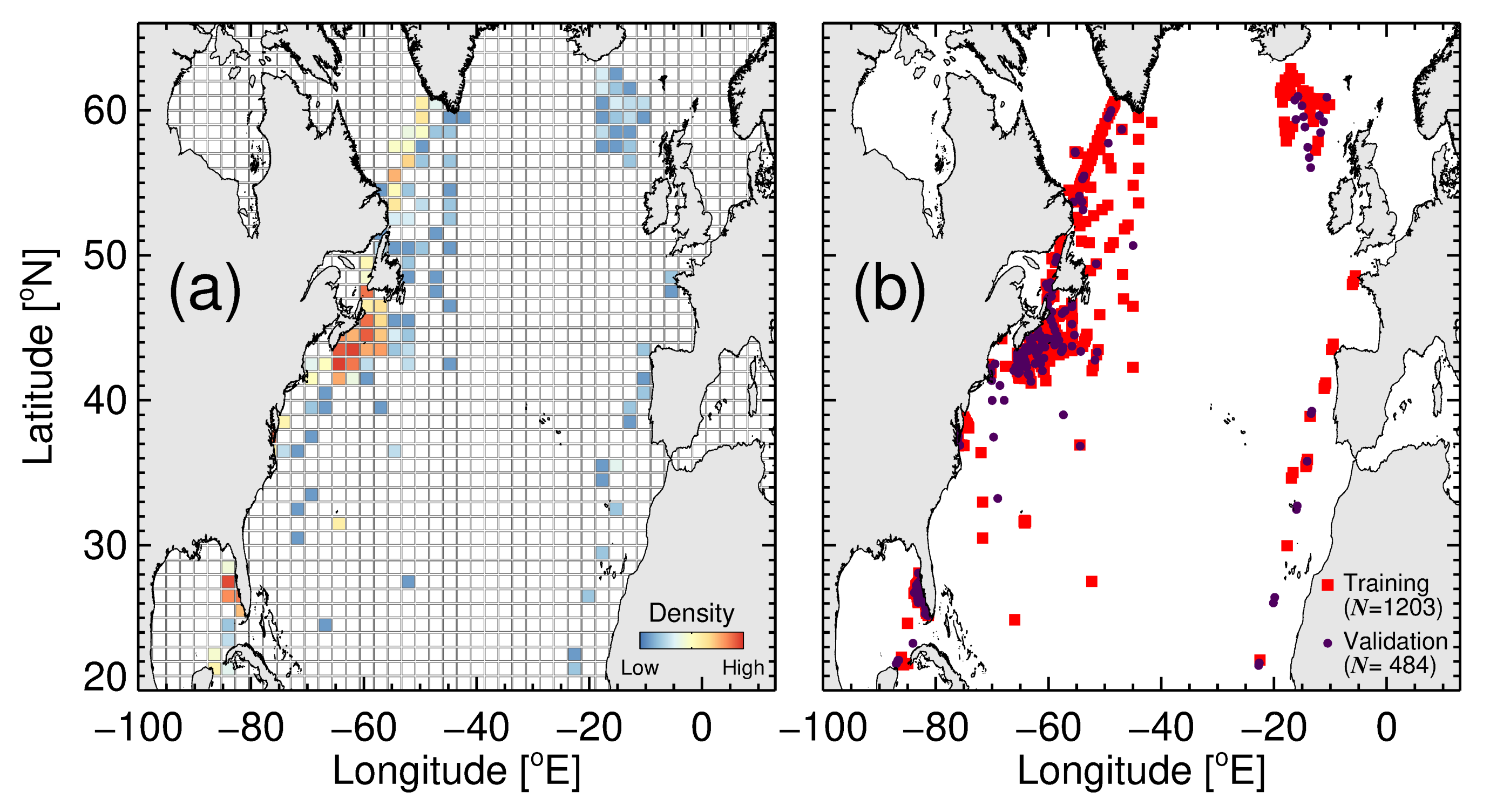
2.2. Data
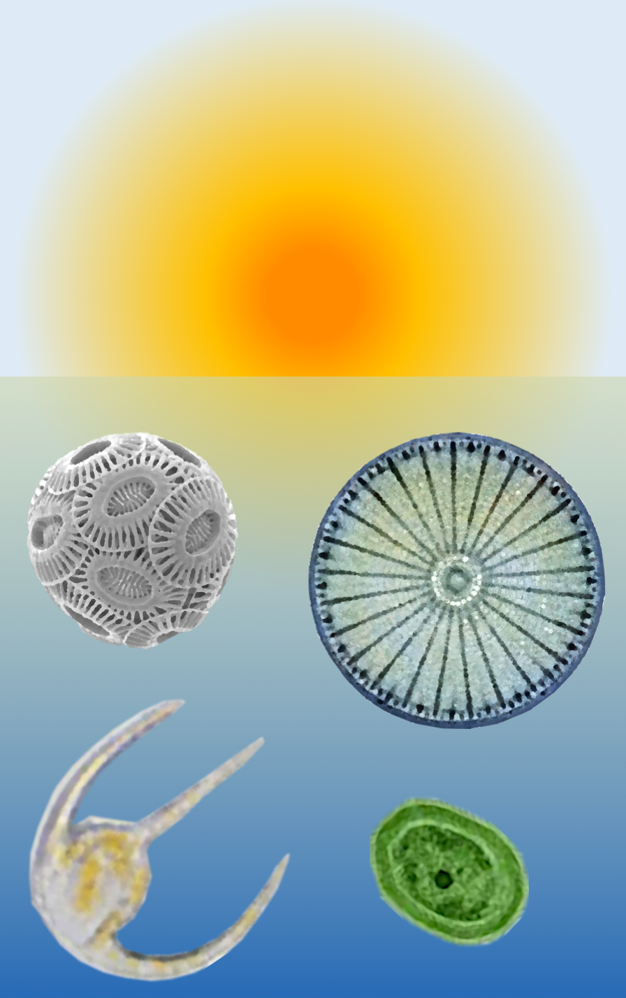
2.3. Four-Population Model of Phytoplankton Absorption
2.4. Other Models That Relate Phytoplankton Absorption to Total Chlorophyll
2.5. Statistical Tests
2.6. Estimation of Uncertainty in Group-Specific
3. Results and Discussion
3.1. Model Tuning
3.2. Model Validation
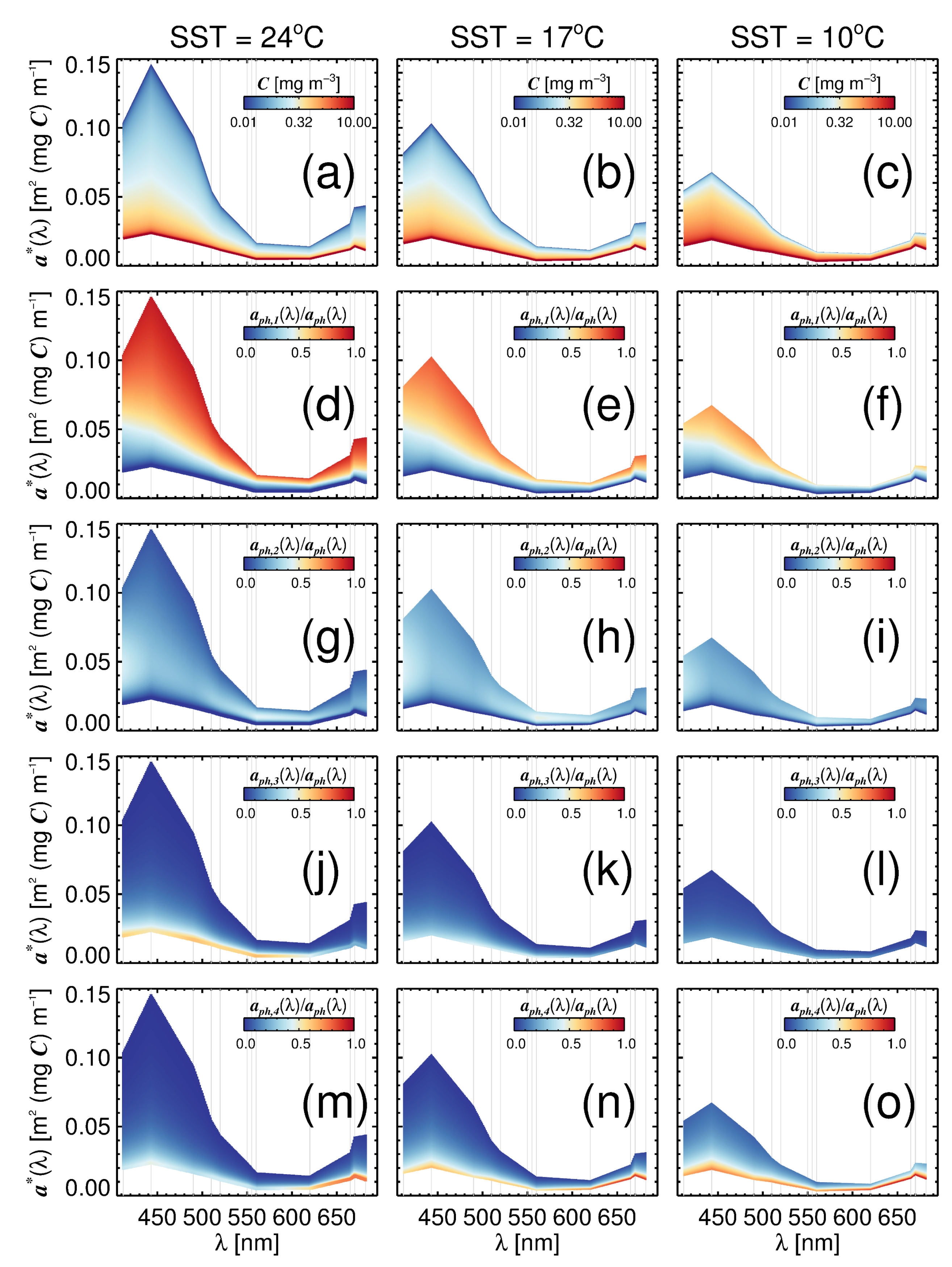
3.3. Variations in with Temperature and Community Structure
3.4. Towards a Mechanistic Understanding of Temperature in the Four-Population Model
3.5. Impact of Variations in on the Blue-to-Green Ratio of Remote-Sensing Reflectance
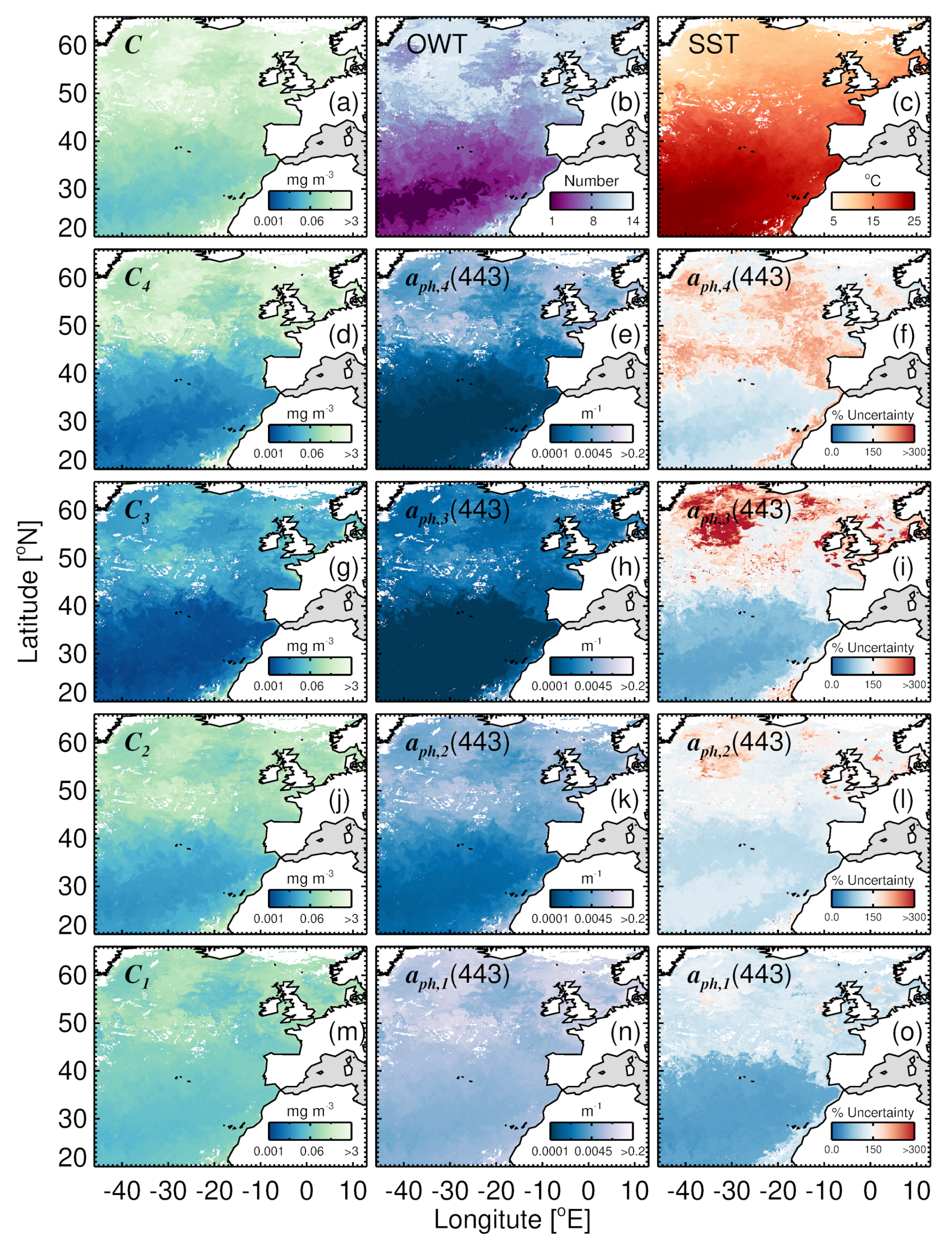
3.6. Mapping Uncertainty in Group-Specific
4. Summary
Author Contributions
Funding
Acknowledgments
Conflicts of Interest
Appendix A. Ocean-Colour Model
Appendix A.1. Remote-Sensing Reflectance
Appendix A.2. Backscattering Model
Appendix A.3. Absorption Model

| Symbol | Definition |
|---|---|
| a | Total absorption coefficient (m) |
| Chlorophyll-specific absorption coefficient of phytoplankton (m [mg C]) | |
| Chlorophyll-specific absorption coefficient of phytoplankton group i, where i can be 1, 2, 3 or 4 (pico-, nano-, dinoflagellates, or diatoms, respectively), or a combination of groups, for example, would represent combined pico- and nano-phytoplankton (m [mg C]) | |
| Absorption coefficient of detrital material (m) | |
| Absorption coefficient of combined detrital particles and coloured dissolved organic matter (m) | |
| Absorption coefficient of particulate matter (m) | |
| Absorption coefficient of phytoplankton (m) | |
| Absorption coefficient of phytoplankton group i, where i can be 1, 2, 3 or 4 (pico-, nano-, dinoflagellates, or diatoms, respectively), or a combination of groups, for example, would represent combined pico- and nano-phytoplankton (m) | |
| Absorption coefficient of pure seawater (m) | |
| Total backscattering coefficient (m) | |
| Backscattering coefficient of particulate matter (m) | |
| Chlorophyll-specific particulate backscattering coefficient of phytoplankton group i, where i can be 1, 2, 3 or 4 (pico-, nano-, dinoflagellates, or diatoms, respectively), or a combination of groups, for example, would represent combined pico- and nano-phytoplankton (m [mg C]) | |
| Constant background particulate backscattering coefficient (m) | |
| Backscattering coefficient of pure seawater (m) | |
| C | Total chlorophyll concentration (mg m) |
| Chlorophyll concentration for phytoplankton group i, where i can be 1, 2, 3 or 4 (pico-, nano-, dinoflagellates, or diatoms, respectively), or a combination of groups, for example, would represent combined pico- and nano-phytoplankton (mg m) | |
| Asymptotic maximum value of (mg m) | |
| Asymptotic maximum value of (mg m) | |
| Fraction of total chlorophyll in combined pico-nanoplankton (cells m) as total chlorophyll tends to zero | |
| Fraction of total chlorophyll in picoplankton (cells m) as total chlorophyll tends to zero | |
| Relative uncertainty (or relative standard deviation) in | |
| Relative uncertainty (or relative standard deviation) in | |
| Relative uncertainty (or relative standard deviation) in | |
| Fraction of total chlorophyll for phytoplankton group i, where i can be 1, 2, 3 or 4 (pico-, nano-, dinoflagellates, or diatoms, respectively), or a combination of groups, for example, would represent combined pico- and nano-phytoplankton | |
| Parameters for Equation (5) controlling changes in with SST, where a, b, c or d depending on parameter (see Table 3) | |
| Parameters for Equation (6) controlling changes in with SST, where a, b, c or d depending on parameter (see Table 3) | |
| Parameters for Equation (7) controlling changes in with SST, where a, b, c or d depending on parameter (see Table 3) | |
| Parameters for Equation (8) controlling changes in with SST, where a, b, c or d depending on parameter (see Table 3) | |
| Parameter for the optical model of Lee et al. [99], see Equation (A1) | |
| Parameter for the optical model of Lee et al. [99], see Equation (A1) | |
| Parameter for the optical model of Lee et al. [99], see Equation (A1) | |
| Parameter for the optical model of Lee et al. [99], see Equation (A1) | |
| r | Pearson correlation coefficient |
| Remote-sensing reflectance (sr) | |
| Slope of an exponential function of with (nm) | |
| SST | Sea surface temperature (C) |
| Parameter of Equation (9) controlling slope of change in with SST (C) | |
| Parameter of Equation (9) controlling the SST mid-point of (C) | |
| Spectral slope of with | |
| Spectral slope of with | |
| Wavelength of light (nm) | |
| Reference wavelength of light (set here to 443 nm) | |
| Collectively representing solar zenith angle, sensor nadir-view angle and sensor azimuth angle, for the optical model of Lee et al. [99], see Equation (A1) | |
| Root mean square error |
References
- Sathyendranath, S.; Gouveia, A.D.; Shetye, S.R.; Ravindran, P.; Platt, T. Biological control of surface temperature in the Arabian Sea. Nature 1991, 349, 54–56. [Google Scholar] [CrossRef]
- Sathyendranath, S.; Platt, T. Spectral effects in bio-optical control on the ocean system. Oceanologia 2007, 49, 5–39. [Google Scholar]
- Kirk, J.T.O. A theoretical analysis of the contribution of algal cells to the attenuation of light within waters, I, General treatment of suspensions of living cells. New Phytol. 1975, 75, 1–20. [Google Scholar]
- Morel, A. Available, usable, and stored radiant energy in relation to marine photosynthesis. Deep Sea Res. 1978, 25, 673–688. [Google Scholar] [CrossRef]
- Morel, A. Optical modelling of the upper ocean in relation to its biogenous matter content (case I waters). J. Geophys. Res. 1988, 93, 10749–10768. [Google Scholar] [CrossRef]
- Sathyendranath, S.; Platt, T. The spectral irradiance field at the surface and interior of the ocean: A model for applications in oceanography and remote sensing. J. Geophys. Res. 1988, 93, 9270–9280. [Google Scholar] [CrossRef]
- Platt, T.; Jassby, A.D. Relationship between photosynthesis and light for natural assemblages of coastal marine-phytoplankton. J. Phycol. 1976, 12, 421–430. [Google Scholar] [CrossRef]
- Kiefer, D.A.; Mitchell, B.G. A simple steady state description of phytoplankton growth based on absorption cross section and quantum efficiency. Limnol. Oceanogr. 1983, 27, 492–499. [Google Scholar] [CrossRef]
- Platt, T.; Sathyendranath, S. Oceanic primary production: Estimation by remote sensing at local and regional Scales. Science 1988, 241, 1613–1620. [Google Scholar] [CrossRef]
- Sathyendranath, S.; Stuart, V.; Cota, G.; Maas, H.; Platt, T. Remote sensing of phytoplankton pigments: A comparison of empirical and theoretical approaches. Int. J. Remote Sens. 2001, 22, 249–273. [Google Scholar] [CrossRef]
- Sathyendranath, S.; Watts, L.; Devred, E.; Platt, T.; Caverhill, C.; Maass, H. Discrimination of diatoms from other phytoplankton using ocean-colour data. Mar. Ecol. Prog. Ser. 2004, 272, 59–68. [Google Scholar] [CrossRef]
- Ciotti, A.M.; Lewis, M.R.; Cullen, J.J. Assessment of the relationships between dominant cell size in natural phytoplankton communities and the spectral shape of the absorption coefficient. Limnol. Oceanogr. 2002, 47, 404–417. [Google Scholar] [CrossRef]
- Roy, S.; Sathyendranath, S.; Platt, T. Retrieval of phytoplankton size from bio-optical measurements: Theory and applications. J. R. Soc. Interface 2010, 8, 650–660. [Google Scholar] [CrossRef] [PubMed]
- Devred, E.; Sathyendranath, S.; Stuart, V.; Platt, T. A three component classification of phytoplankton absorption spectra: Applications to ocean-colour data. Remote Sens. Environ. 2011, 115, 2255–2266. [Google Scholar] [CrossRef]
- Dall’Olmo, G.; Boss, E.; Behrenfeld, M.; Westberry, T.K. Particulate optical scattering coefficients along an Atlantic Meridional Transect. Opt. Express 2012, 20, 21532–21551. [Google Scholar] [CrossRef] [PubMed]
- Organelli, E.; Bricaud, A.; Antoine, D.; Uitz, J. Multivariate approach for the retrieval of phytoplankton size structure from measured light absorption spectra in the Mediterranean Sea (BOUSSOLE site). Appl. Opt. 2013, 52, 2257–2273. [Google Scholar] [CrossRef]
- Kirk, J.T.O. A theoretical analysis of the contribution of algal cells to the attenuation of light within waters, II, Spherical cells. New Phytol. 1975, 75, 21–36. [Google Scholar] [CrossRef]
- Morel, A.; Bricaud, A. Theoretical results concerning light absorption in a discrete medium, and application to specific absorption of phytoplankton. Deep-Sea Res. 1981, 28, 1375–1393. [Google Scholar] [CrossRef]
- Sathyendranath, S.; Lazzara, L.; Prieur, L. Variations in the spectral values of specific absorption of phytoplankton. Limnol. Oceanogr. 1987, 32, 403–415. [Google Scholar] [CrossRef]
- Hoepffner, N.; Sathyendranath, S. Effect of pigment composition on absorption properties of phytoplankton. Mar. Ecol. Prog. Ser. 1991, 73, 11–23. [Google Scholar] [CrossRef]
- Lohrenz, S.E.; Weidemann, A.D.; Tuel, M. Phytoplankton spectral absorption as influenced by community size structure and pigment composition. J. Plankton Res. 2003, 25, 35–61. [Google Scholar] [CrossRef]
- Bricaud, A.; Claustre, H.; Ras, J.; Oubelkheir, K. Natural variability of phytoplanktonic absorption in oceanic waters: Influence of the size structure of algal populations. J. Geophys. Res. 2004, 109, C11010. [Google Scholar] [CrossRef]
- Bricaud, A.; Babin, M.; Morel, A.; Claustre, H. Variability in the chlorophyll specific absorption coefficients of natural phytoplankton: Analysis and parameterization. J. Geophys. Res. 1995, 100, 13321–13332. [Google Scholar] [CrossRef]
- Prieur, L.; Sathyendranath, S. An optical classification of coastal and oceanic waters based on the specific spectral absorption curves of phytoplankton pigments, dissolved organic matter and other particulate materials. Limnol. Oceanogr. 1981, 26, 617–689. [Google Scholar] [CrossRef]
- Yentch, C.; Phinney, D. A bridge between ocean optics and microbial ecology. Limnol. Oceanogr. 1989, 34, 1694–1705. [Google Scholar] [CrossRef]
- Morel, A. Light and marine photosynthesis: A spectral model with geochemical and climatological implications. Prog. Oceanogr. 1991, 26, 263–306. [Google Scholar] [CrossRef]
- Bricaud, A.; Morel, A.; Babin, M.; Allali, K.; Claustre, H. Variations of light absorption by suspended particles with the chlorophyll a concentration in oceanic (case 1) waters: Analysis and implications for bio-optical models. J. Geophys. Res. 1998, 103, 31033–31044. [Google Scholar] [CrossRef]
- Carder, K.L.; Hawes, S.K.; Baker, K.A.; Smith, R.C.; Steward, R.G.; Mitchell, B.G. Reflectance model for quantifying chlorophyll a in the presence of productivity degradation products. J. Geophys. Res. 1991, 96, 20599–20611. [Google Scholar] [CrossRef]
- Cleveland, J.S. Regional models for phytoplankton absorption as a function of chlorophyll a concentration. J. Geophys. Res. Ocean. 1995, 100, 13333–13344. [Google Scholar] [CrossRef]
- Lutz, V.A.; Sathyendranath, S.; Head, E.J.H. Absorption coefficient of phytoplankton: Regional variations in the North Atlantic. Mar. Ecol. Prog. Ser. 1996, 135, 197–213. [Google Scholar] [CrossRef]
- Brewin, R.J.W.; Devred, E.; Sathyendranath, S.; Hardman-Mountford, N.J.; Lavender, S.J. Model of phytoplankton absorption based on three size classes. Appl. Opt. 2011, 50, 4535–4549. [Google Scholar] [CrossRef]
- Devred, E.; Sathyendranath, S.; Stuart, V.; Maas, H.; Ulloa, O.; Platt, T. A two-component model of phytoplankton absorption in the open ocean: Theory and applications. J. Geophys. Res. 2006, 111, C03011. [Google Scholar] [CrossRef]
- Uitz, J.; Huot, Y.; Bruyant, F.; Babin, M.; Claustre, H. Relating phytoplankton photophysiological properties to community structure on large scales. Limnol. Oceanogr. 2008, 53, 614–630. [Google Scholar] [CrossRef]
- Brewin, R.J.W.; Sathyendranath, S.; Hirata, T.; Lavender, S.J.; Barciela, R.; Hardman-Mountford, N.J. A three-component model of phytoplankton size class for the Atlantic Ocean. Ecol. Model. 2010, 221, 1472–1483. [Google Scholar] [CrossRef]
- Kamykowski, D.; Zentara, S.J. Can phytoplankton community structure be inferred from satellite-derived sea surface temperature anomalies calculated relative to nitrate depletion temperatures? Remote Sens. Environ. 2003, 86, 444–457. [Google Scholar] [CrossRef]
- Raitsos, D.E.; Lavender, S.J.; Maravelias, C.D.; Haralambous, J.; Richardson, A.J.; Reid, P.C. Identifying four phytoplankton functional types from space: An ecological approach. Limnol. Oceanogr. 2008, 53, 605–613. [Google Scholar] [CrossRef]
- Feng, Y.; Hare, C.E.; Leblanc, K.; Rose, J.M.; Zhang, Y.; DiTullio, G.R.; Lee, P.A.; Wilhelm, S.W.; Rowe, J.M.; Sun, J.; et al. Effects of increased pCO2 and temperature on the North Atlantic spring bloom. I. The phytoplankton community and biogeochemical response. Mar. Ecol. Prog. Ser. 2009, 388, 13–25. [Google Scholar] [CrossRef]
- Morán, X.A.G.; López-Urrutia, A.; Calvo-Díaz, A.; Li, W.K.W. Increasing importance of small phytoplankton in a warmer ocean. Glob. Chang. Biol. 2010, 16, 1137–1144. [Google Scholar] [CrossRef]
- Barnes, C.; Irigoien, X.; De Oliveira, J.A.A.; Maxwell, D.; Jennings, S. Predicting marine phytoplankton community size structure from empirical relationships with remotely sensed variables. J. Plankton Res. 2011, 33, 13–24. [Google Scholar] [CrossRef]
- Hilligsøe, K.M.; Richardson, K.; Bendtsen, J.; Sørensen, L.L.; Nielsen, T.G.; Lyngsgaard, M.M. Linking phytoplankton community size composition with temperature, plankton food web structure and sea–air CO2 flux. Deep Sea Res. Part I Oceanogr. Res. Pap. 2011, 58, 826–838. [Google Scholar] [CrossRef]
- Flombaum, P.; Gallegos, J.L.; Gordillo, R.A.; Rincón, J.; Zabala, L.L.; Jiao, N.; Karl, D.M.; Li, W.; Lomas, M.; Veneziano, D.; et al. Present and future global distributions of the marine Cyanobacteria Prochlorococcus synechococcus. Proc. Natl. Acad. Sci. USA 2013, 110, 9824–9829. [Google Scholar] [CrossRef] [PubMed]
- Mousing, E.A.; Ellegaard, M.; Richardson, K. Global patterns in phytoplankton community size structure–evidence for a direct temperature effect. Mar. Ecol. Prog. Ser. 2014, 496, 25–38. [Google Scholar] [CrossRef]
- Lange, P.; Brewin, R.J.W.; Dall’Olmo, G.; Tarran, G.; Sathyendranath, S.; Zubkov, M.; Bouman, H. Scratching beneath the surface: A model to predict the vertical distribution of Prochlorococcus Using Remote Sensing. Remote Sens. 2018, 10, 847. [Google Scholar] [CrossRef]
- Agusti, S.; Lubián, L.M.; Morerno-Ostos, E.; Estrada, M.; Duarte, C.M. Projected Changes in Photosynthetic Picoplankton in a Warmer Subtropical Ocean. Front. Mar. Sci. 2019, 5, 506. [Google Scholar] [CrossRef]
- Bouman, H.A.; Platt, T.; Sathyendranath, S.; Li, W.K.; Stuart, V.; Fuentes-Yaco, C.; Maass, H.; Horne, E.P.; Ulloa, O.; Lutz, V.; et al. Temperature as indicator of optical properties and community structure of marine phytoplankton: Implications for remote sensing. Mar. Ecol. Prog. Ser. 2003, 258, 19–30. [Google Scholar] [CrossRef]
- Brewin, R.J.W.; Ciavatta, S.; Sathyendranath, S.; Jackson, T.; Tilstone, G.; Curran, K.; Airs, R.; Cummings, D.; Brotas, V.; Organelli, E.; et al. Uncertainty in ocean-color estimates of chlorophyll for phytoplankton groups. Front. Mar. Sci. 2017, 4, 104. [Google Scholar] [CrossRef]
- Ciavatta, S.; Brewin, R.J.W.; Skákala, J.; Polimene, L.; de Mora, L.; Artioli, Y.; Allen, J.I. Assimilation of ocean-color plankton functional types to improve marine ecosystem simulations. J. Geophys. Res. Ocean. 2018, 123, 834–854. [Google Scholar] [CrossRef]
- Skákala, J.; Ford, D.; Brewin, R.J.W.; McEwan, R.; Kay, S.; Taylor, B.; de Mora, L.; Ciavatta, S. The assimilation of phytoplankton functional types for operational forecasting in the northwest European shelf. J. Geophys. Res. Ocean. 2018, 123, 5230–5247. [Google Scholar] [CrossRef]
- Ciavatta, S.; Torres, R.; Martinez-Vicente, V.; Smyth, T.; Dall’Olmo, G.; Polimene, L.; Allen, J.I. Assimilation of remotely-sensed optical properties to improve marine biogeochemistry modelling. Prog. Oceanogr. 2014, 127, 74–95. [Google Scholar] [CrossRef]
- Ducklow, H.W.; Harris, R.P. Introduction to the JGOFS North Atlantic bloom experiment. Deep Sea Res. Part II Top. Stud. Oceanogr. 1993, 40, 1–8. [Google Scholar] [CrossRef]
- Holt, J.; Allen, J.I.; Anderson, T.R.; Brewin, R.J.W.; Butenschön, M.; Harle, J.; Huse, G.; Lehodey, P.; Lindemann, C.; Memery, L.; et al. Challenges in integrative approaches to modelling the marine ecosystems of the North Atlantic: Physics to fish and coasts to ocean. Prog. Oceanogr. 2014, 129, 285–313. [Google Scholar] [CrossRef]
- Werdell, P.J.; Bailey, S.W. An improved in-situ bio-optical data set for ocean colour algorithm development and satellite data production validation. Remote Sens. Environ. 2005, 98, 122–140. [Google Scholar] [CrossRef]
- Werdell, P.J. Global bio-optical algorithms for ocean color satellite applications. EOS Trans. AGU 2009, 90, 4. [Google Scholar] [CrossRef]
- De Boyer Montégut, C.; Madec, G.; Fisher, A.S.; Lazar, A.; Ludicone, D. Mixed layer depth over the global ocean: An examination of profile data and a profile-based climatology. J. Geophys. Res. 2004, 109, C12003. [Google Scholar] [CrossRef]
- Reynolds, R.W.; Smith, T.M.; Liu, C.; Chelton, D.B.; Casey, K.S.; Schlax, M.G. Daily high-resolution-blended analysis for sea surface temperature. J. Clim. 2007, 20, 5473–5496. [Google Scholar] [CrossRef]
- Moré, J. The Levenberg-Marquardt algorithm: Implementation and theory. In Numerical Analysis; Springer: Berlin, Germany, 1978; p. 105. [Google Scholar]
- Markwardt, C.B. Non-linear least squares fitting in IDL with MPFIT. In Proceedings of the Astronomical Data Analysis Software and Systems XVIII, ASP Conference Series, Quebec City, QC, Canada, 2–5 November 2008; Bohlender, D., Dowler, P., Duran, D., Eds.; Astronomical Society of the Pacific: San Francisco, CA, USA, 2008; Volume 411. [Google Scholar]
- Efron, B. Bootstrap methods: Another look at the jackknife. Ann. Stat. 1979, 7, 1–26. [Google Scholar] [CrossRef]
- Brewin, R.J.W.; Sathyendranath, S.; Jackson, T.; Barlow, R.; Brotas, V.; Airs, R.; Lamont, T. Influence of light in the mixed layer on the parameters of a three-component model of phytoplankton size structure. Remote Sens. Environ. 2015, 168, 437–450. [Google Scholar] [CrossRef]
- Campbell, J.W. The lognormal distribution as a model for bio-optical variability in the sea. J. Geophys. Res. 1995, 100, 13237–13254. [Google Scholar] [CrossRef]
- Jackson, T.; Sathyendranath, S.; Mélin, F. An improved optical classification scheme for the Ocean Colour Essential Climate Variable and its applications. Remote Sens. Environ. 2017, 203, 152–161. [Google Scholar] [CrossRef]
- Ciavatta, S.; Kay, S.; Saux-Picart, S.; Butenschön, M.; Allen, J.I. Decadal reanalysis of biogeochemical indicators and fluxes in the North West European shelf-sea ecosystem. J. Geophys. Res. 2016, 121, 1824–1845. [Google Scholar] [CrossRef]
- Duysens, L.N.M. The flattening of the absorption spectrum of suspensions as compared to that of solutions. Biochim. Biophys. Acta 1956, 19, 1–12. [Google Scholar] [CrossRef]
- Organelli, E.; Nuccio, C.; Lazzara, L.; Uitz, J.; Bricaud, A.; Massi, L. On the discrimination of multiple phytoplankton groups from light absorption spectra of assemblages with mixed taxonomic composition and variable light conditions. Appl. Opt. 2017, 56, 3952–3968. [Google Scholar] [CrossRef]
- Ciotti, A.M.; Bricaud, A. Retrievals of a size parameter for phytoplankton and spectral light absorption by coloured detrital matter from water-leaving radiances at SeaWiFS channels in a continental shelf off Brazil. Limnol. Oceanogr. Methods 2006, 4, 237–253. [Google Scholar] [CrossRef]
- Barlow, R.G.; Aiken, J.; Holligan, P.M.; Cummings, D.G.; Mariotena, S.; Hooker, S. Phytoplankton pigment and absorption characteristics along meridional transects in the Atlantic Ocean. Deep-Sea Res. I 2002, 49, 637–660. [Google Scholar] [CrossRef]
- Partensky, F.; Hoepffner, N.; Li, W.K.W.; Ulloa, O.; Vaulot, D. Photoacclimation of Prochlorococcus sp. (Prochlorophyta) strains isolated from the North Atlantic and the Mediterranean Sea. Plant Physiol. 1993, 101, 285–296. [Google Scholar] [CrossRef]
- Morel, A.; Ahn, Y.H.; Partensky, F.; Vaulot, D.; Claustre, H. Prochlorococcus Synechococcus: A comparitive study of thier optical properties in relation to thier size and pigmentation. J. Mar. Res. 1993, 51, 617–649. [Google Scholar] [CrossRef]
- Moore, L.R.; Goericke, R.; Chisholm, S.W. Comparative physiology of Synechococcus and Prochlorococcus: Influence of light and temperature on growth, pigments, fluorescence and absorptive properties. Mar. Ecol. Prog. Ser. 1995, 116, 259–275. [Google Scholar] [CrossRef]
- Liu, H.; Probert, I.; Uitz, J.; Claustre, H.; Aris-Brosou, S.; Frada, M.; Not, F.; de Vargas, C. Extreme diversity in noncalcifying haptophytes explains a major pigment paradox in open oceans. Proc. Natl. Acad. Sci. USA 2009, 106, 12803–12808. [Google Scholar] [CrossRef]
- Johnsen, G.; Nelson, N.B.; Jovine, R.V.M.; Prézelin, B.B. Chromoprotein- and pigment-dependent modelling of spectral light absorption in two dinoflagellates, Prorocentrum minimum and Heterocapsa pygmaea. Mar. Ecol. Prog. Ser. 1994, 114, 245–258. [Google Scholar] [CrossRef]
- Finkel, Z.V. Light absorption and size scaling of light-limited metabolism in marine diatoms. Limnol. Oceanogr. 2001, 38, 679–687. [Google Scholar] [CrossRef]
- Hirata, T.; Aiken, J.; Hardman-Mountford, N.J.; Smyth, T.J.; Barlow, R.G. An absorption model to derive phytoplankton size classes from satellite ocean colour. Remote Sens. Environ. 2008, 112, 3153–3159. [Google Scholar] [CrossRef]
- Werdell, P.J.; Franz, B.A.; Bailey, S.W.; Feldman, G.C.; Boss, E.; Brando, V.E.; Dowell, M.; Hirata, T.; Lavender, S.J.; Lee, Z.; et al. Generalized ocean color inversion model for retrieving marine inherent optical properties. Appl. Opt. 2013, 52, 2019–2037. [Google Scholar] [CrossRef]
- IOCCG. Inherent Optical Property Measurements and Protocols: Absorption Coefficient. In IOCCG Ocean Optics and Biogeochemistry Protocols for Satellite Ocean Colour Sensor Validation; Neeley, A.R., Mannino, A., Eds.; IOCCG: Dartmouth, NS, Canada, 2018; Volume 1. [Google Scholar]
- Brewin, R.J.W.; Sathyendranath, S.; Müller, D.; Brockmann, C.; Deschamps, P.Y.; Devred, E.; Doerffer, R.; Fomferra, N.; Franz, B.A.; Grant, M.; et al. The Ocean Colour Climate Change Initiative: III. A round-robin comparison on in-water bio-optical algorithms. Remote Sens. Environ. 2015, 162, 271–294. [Google Scholar] [CrossRef]
- Marañón, E.; Cermeño, P.; Latasa, M.; Tadonléké, R.D. Temperature, resources, and phytoplankton size structure in the ocean. Limnol. Oceanogr. 2012, 57, 1266–1278. [Google Scholar] [CrossRef]
- López-Urrutia, A.; Morán, X.A.G. Temperature affects the size-structure of phytoplankton communities in the ocean. Limnol. Oceanogr. 2015, 60, 733–738. [Google Scholar] [CrossRef]
- Marañón, E.; Cermeno, P.; Latasa, M.; Tadonléké, R.D. Resource supply alone explains the variability of marine phytoplankton size structure. Limnol. Oceanogr. 2015, 60, 1848–1854. [Google Scholar] [CrossRef]
- Eppley, R.W. Temperature and phytoplankton growth in the sea. Fish. Bull. 1972, 70, 1063–1085. [Google Scholar]
- Aksnes, D.L.; Egge, J.K. A theoretical-model for nutrient-uptake in phytoplankton. Mar. Ecol. Prog. Ser. 1991, 70, 65–72. [Google Scholar] [CrossRef]
- Toseland, A.; Daines, S.J.; Clark, J.R.; Kirkham, A.; Strauss, J.; Uhlig, C.; Lenton, T.M.; Valentin, K.; Pearson, G.A.; Moulton, V.; et al. The impact of temperature on marine phytoplankton resource allocation and metabolism. Nat. Clim. Chang. 2013, 3, 979–984. [Google Scholar] [CrossRef]
- Brewin, R.J.W.; Sathyendranath, S.; Tilstone, G.; Lange, P.K.; Platt, T. A multicomponent model of phytoplankton size structure. J. Geophys. Res. Ocean. 2014, 119, 3478–3496. [Google Scholar] [CrossRef]
- López-Urrutia, A. The metabolic theory of ecology and algal bloom formation. Limnol. Oceanogr. 2008, 53, 2046–2047. [Google Scholar] [CrossRef]
- Sathyendranath, S.; Platt, T.; Horne, E.P.; Harrison, W.G.; Ulloa, O.; Outerbridge, R.; Hoepffner, N. Estimation of new production in the ocean by compound remote sensing. Nature 1991, 353, 129–133. [Google Scholar] [CrossRef]
- Ward, B.A. Temperature-correlated changes in phytoplankton community structure are restricted to polar waters. PLoS ONE 2015, 10, e0135581. [Google Scholar] [CrossRef]
- Brewin, R.J.W.; Morán, X.A.G.; Raitsos, D.E.; Gittings, J.A.; Calleja, M.L.; Viegas, M.S.; Ansari, M.I.; Al-Otaibi, N.; Huete-Stauffer, T.M.; Hoteit, I. Factors regulating the relationship between total and size-fractionated chlorophyll-a in coastal waters of the Red Sea. Front. Microbiol. 2019, 10, 1964. [Google Scholar] [CrossRef]
- O’Reilly, J.E.; Maritorena, S.; Mitchell, B.G.; Siegel, D.A.; Carder, K.L.; Garver, S.A.; Kahru, M.; McClain, C. Ocean chlorophyll algorithms for SeaWiFS. J. Geophys. Res. 1998, 103, 24937–24953. [Google Scholar] [CrossRef]
- NASA. Ocean Color Chlorophyll (OC) v6. 2010. Available online: http://oceancolor.gsfc.nasa.gov/REPROCESSING/R2009/ocv6/ (accessed on 25 September 2019).
- Gregg, W.W.; Casey, N.W. Global and regional evaluation of the SeaWiFS chlorophyll data set. Remote Sens. Environ. 2004, 93, 463–479. [Google Scholar] [CrossRef]
- Johnson, R.; Strutton, P.G.; Wright, S.W.; McMinn, A.; Meiners, K.M. Three improved satellite chlorophyll algorithms for the Southern Ocean. J. Geophys. Res. Ocean. 2013, 118, 3694–3703. [Google Scholar] [CrossRef]
- Jena, B. The effect of phytoplankton pigment composition and packaging on the retrieval of chlorophyll-a concentration from satellite observations in the Southern Ocean. Int. J. Remote Sens. 2017, 38, 3763–3784. [Google Scholar] [CrossRef]
- Christensen, J.H.; Hewitson, B.; Busuioc, A.; Chen, A.; Gao, X.; Held, I.; Jones, R.; Kolli, R.K.; Kwon, W.T.; Laprise, R.; et al. Regional Climate Projections. In Climate Change 2007: The Physical Science Basis. Contribution of Working Group I to the Fourth Assessment Report of the Intergovernmental Panel on Climate; Solomon, S., Qin, D., Manning, M., Chen, Z., Marquis, M., Averyt, K.B., Tignor, M., Miller, H.L., Eds.; Cambridge University Press: Cambridge, UK; New York, NY, USA, 2007. [Google Scholar]
- Dutkiewicz, S.; Hickman, A.E.; Jahn, O.; Henson, S.; Beaulieu, C.; Monier, E. Ocean colour signature of climate change. Nat. Commun. 2019, 10, 1–13. [Google Scholar] [CrossRef]
- Brewin, R.J.W.; Dall’Olmo, G.; Pardo, S.; van Dongen-Vogel, V.; Boss, E.S. Underway spectrophotometry along the Atlantic Meridional Transect reveals high performance in satellite chlorophyll retrievals. Remote Sens. Environ. 2016, 183, 82–97. [Google Scholar] [CrossRef]
- Gregg, W.W.; Rousseaux, C.S. Directional and spectral irradiance in ocean models: Effects on simulated global phytoplankton, nutrients, and primary production. Front. Mar. Sci. 2016, 3, 240. [Google Scholar] [CrossRef]
- Shulman, I.; Frolov, S.; Anderson, S.; Penta, B.; Gould, R.; Sakalaukus, P.; Ladner, S. Impact of bio-optical data assimilation on short-term coupled physical, bio-optical model predictions. J. Geophys. Res. Ocean. 2013, 118, 2215–2230. [Google Scholar] [CrossRef]
- Jones, E.M.; Baird, M.E.; Mongin, M.; Parslow, J.; Skerratt, J.; Lovell, J.; Margvelashvili, N.; Matear, R.J.; Wild-Allen, K.; Robson, B.; et al. Use of remote-sensing reflectance to constrain a data assimilating marine biogeochemical model of the Great Barrier Reef. Biogeosciences 2016, 13, 6441–6469. [Google Scholar] [CrossRef]
- Lee, Z.P.; Du, K.; Voss, K.J.; Zibordi, G.; Lubac, B.; Arnone, R.; Weidemann, A. An inherent-optical- property-centered approach to correct the angular effects in water-leaving radiance. Appl. Opt. 2011, 50, 3155–3167. [Google Scholar] [CrossRef]
- Zhang, X.; Hu, L. Estimating scattering of pure water from density fluctuation of the refractive index. Opt. Express 2009, 17, 1671–1678. [Google Scholar] [CrossRef]
- Zhang, X.; Hu, L.; He, M.X. Scattering by pure seawater: Effect of salinity. Opt. Express 2009, 17, 5698–5710. [Google Scholar] [CrossRef]
- Brewin, R.J.W.; Dall’Olmo, G.; Sathyendranath, S.; Hardman-Mountford, N.J. Particle backscattering as a function of chlorophyll and phytoplankton size structure in the open-ocean. Opt. Express 2012, 20, 17632–17652. [Google Scholar] [CrossRef]
- Pope, R.; Fry, E. Absorption spectrum (380-700 nm) of pure water. II. Integrating cavity measurements. Appl. Opt. 1997, 36, 8710–8723. [Google Scholar] [CrossRef]
- Morel, A.; Gentili, B. A simple band ratio technique to quantify the colored dissolved and detrital organic material from ocean color remotely sensed data. Remote Sens. Environ. 2009, 113, 998–1011. [Google Scholar] [CrossRef]


| Model Parameter | Parameters Values $ | |||
|---|---|---|---|---|
| (Equation (5)) | ||||
| (−1.57↔ −1.43) | (−1.41↔ −1.25) | (14.87↔15.05) | (0.23↔0.26) | |
| (Equation (6)) | ||||
| (0.28↔0.30) | (2.87↔3.26) | (16.19↔16.29) | (0.55↔0.57) | |
| (Equation (7)) | ||||
| (0.367↔0.373) | (1.10↔1.16) | (14.87↔14.91) | (0.566↔0.571) | |
| (Equation (8)) | ||||
| (0.501↔0.505) | (1.31↔1.37) | 17.28↔17.32) | (0.256↔0.259) | |
| Wavelength | Picophytoplankton | Nanophytoplankton | Dinoflagellates | Diatoms |
|---|---|---|---|---|
| (nm) | ||||
| 412 | 0.124 (±0.054) | 0.052 (±0.031) | 0.039 (±0.014) | 0.011 (±0.004) |
| 443 | 0.183 (±0.043) | 0.039 (±0.027) | 0.041 (±0.016) | 0.016 (±0.005) |
| 490 | 0.118 (±0.025) | 0.022 (±0.018) | 0.035 (±0.008) | 0.009 (±0.003) |
| 510 | 0.067 (±0.020) | 0.018 (±0.015) | 0.026 (±0.005) | 0.008 (±0.003) |
| 520 | 0.053 (±0.016) | 0.016 (±0.013) | 0.022 (±0.004) | 0.007 (±0.002) |
| 550 | 0.028 (±0.010) | 0.011 (±0.008) | 0.013 (±0.002) | 0.004 (±0.001) |
| 555 | 0.023 (±0.009) | 0.011 (±0.007) | 0.012 (±0.002) | 0.003 (±0.001) |
| 560 | 0.018 (±0.008) | 0.011 (±0.006) | 0.010 (±0.002) | 0.003 (±0.001) |
| 620 | 0.016 (±0.007) | 0.007 (±0.005) | 0.008 (±0.001) | 0.004 (±0.001) |
| 665 | 0.037 (±0.010) | 0.009 (±0.008) | 0.010 (±0.006) | 0.013 (±0.002) |
| 670 | 0.052 (±0.013) | 0.011 (±0.010) | 0.011 (±0.008) | 0.015 (±0.002) |
| 682 | 0.054 ±0.013) | 0.012 (±0.009) | 0.009 (±0.008) | 0.012 (±0.002) |
| Wavelength (nm) | In Situ Chlorophyll-a as Input * | Satellite Chlorophyll-a as Input * | ||||||||||
|---|---|---|---|---|---|---|---|---|---|---|---|---|
| This Study | Brewin et al. [31] | Bricaud et al. [23] | This Study | Brewin et al. [31] | Bricaud et al. [23] | |||||||
| 412 | 0.89 | 0.21 | 0.88 | 0.23 | 0.89 | 0.26 | 0.80 | 0.28 | 0.80 | 0.31 | 0.80 | 0.34 |
| 443 | 0.87 | 0.22 | 0.86 | 0.22 | 0.87 | 0.25 | 0.78 | 0.27 | 0.78 | 0.29 | 0.78 | 0.32 |
| 490 | 0.87 | 0.21 | 0.86 | 0.21 | 0.86 | 0.22 | 0.77 | 0.27 | 0.78 | 0.27 | 0.78 | 0.29 |
| 510 | 0.89 | 0.21 | 0.89 | 0.21 | 0.89 | 0.22 | 0.79 | 0.28 | 0.80 | 0.29 | 0.80 | 0.30 |
| 520 | 0.90 | 0.21 | 0.90 | 0.21 | 0.91 | 0.22 | 0.80 | 0.29 | 0.81 | 0.30 | 0.81 | 0.31 |
| 550 | 0.90 | 0.26 | 0.90 | 0.25 | 0.91 | 0.24 | 0.80 | 0.34 | 0.80 | 0.36 | 0.81 | 0.33 |
| 555 | 0.90 | 0.26 | 0.89 | 0.26 | 0.91 | 0.24 | 0.80 | 0.35 | 0.80 | 0.37 | 0.81 | 0.34 |
| 560 | 0.90 | 0.27 | 0.89 | 0.27 | 0.91 | 0.24 | 0.80 | 0.35 | 0.80 | 0.38 | 0.82 | 0.33 |
| 620 | 0.91 | 0.25 | 0.91 | 0.23 | 0.91 | 0.23 | 0.79 | 0.36 | 0.80 | 0.35 | 0.81 | 0.34 |
| 665 | 0.92 | 0.22 | 0.92 | 0.22 | 0.92 | 0.21 | 0.80 | 0.34 | 0.81 | 0.33 | 0.81 | 0.34 |
| 670 | 0.91 | 0.23 | 0.92 | 0.22 | 0.92 | 0.22 | 0.79 | 0.34 | 0.80 | 0.33 | 0.80 | 0.34 |
| 682 | 0.88 | 0.29 | 0.89 | 0.26 | 0.89 | 0.26 | 0.76 | 0.39 | 0.78 | 0.37 | 0.78 | 0.37 |
© 2019 by the authors. Licensee MDPI, Basel, Switzerland. This article is an open access article distributed under the terms and conditions of the Creative Commons Attribution (CC BY) license (http://creativecommons.org/licenses/by/4.0/).
Share and Cite
Brewin, R.J.W.; Ciavatta, S.; Sathyendranath, S.; Skákala, J.; Bruggeman, J.; Ford, D.; Platt, T. The Influence of Temperature and Community Structure on Light Absorption by Phytoplankton in the North Atlantic. Sensors 2019, 19, 4182. https://doi.org/10.3390/s19194182
Brewin RJW, Ciavatta S, Sathyendranath S, Skákala J, Bruggeman J, Ford D, Platt T. The Influence of Temperature and Community Structure on Light Absorption by Phytoplankton in the North Atlantic. Sensors. 2019; 19(19):4182. https://doi.org/10.3390/s19194182
Chicago/Turabian StyleBrewin, Robert J. W., Stefano Ciavatta, Shubha Sathyendranath, Jozef Skákala, Jorn Bruggeman, David Ford, and Trevor Platt. 2019. "The Influence of Temperature and Community Structure on Light Absorption by Phytoplankton in the North Atlantic" Sensors 19, no. 19: 4182. https://doi.org/10.3390/s19194182
APA StyleBrewin, R. J. W., Ciavatta, S., Sathyendranath, S., Skákala, J., Bruggeman, J., Ford, D., & Platt, T. (2019). The Influence of Temperature and Community Structure on Light Absorption by Phytoplankton in the North Atlantic. Sensors, 19(19), 4182. https://doi.org/10.3390/s19194182