An Ocean-Colour Time Series for Use in Climate Studies: The Experience of the Ocean-Colour Climate Change Initiative (OC-CCI)

 ,
,  ,
,  ,
,  , , , , , , , , , , , , , , , ,
  , , ,
, , , 
Abstract
1. Introduction
2. User Consultation
3. Data
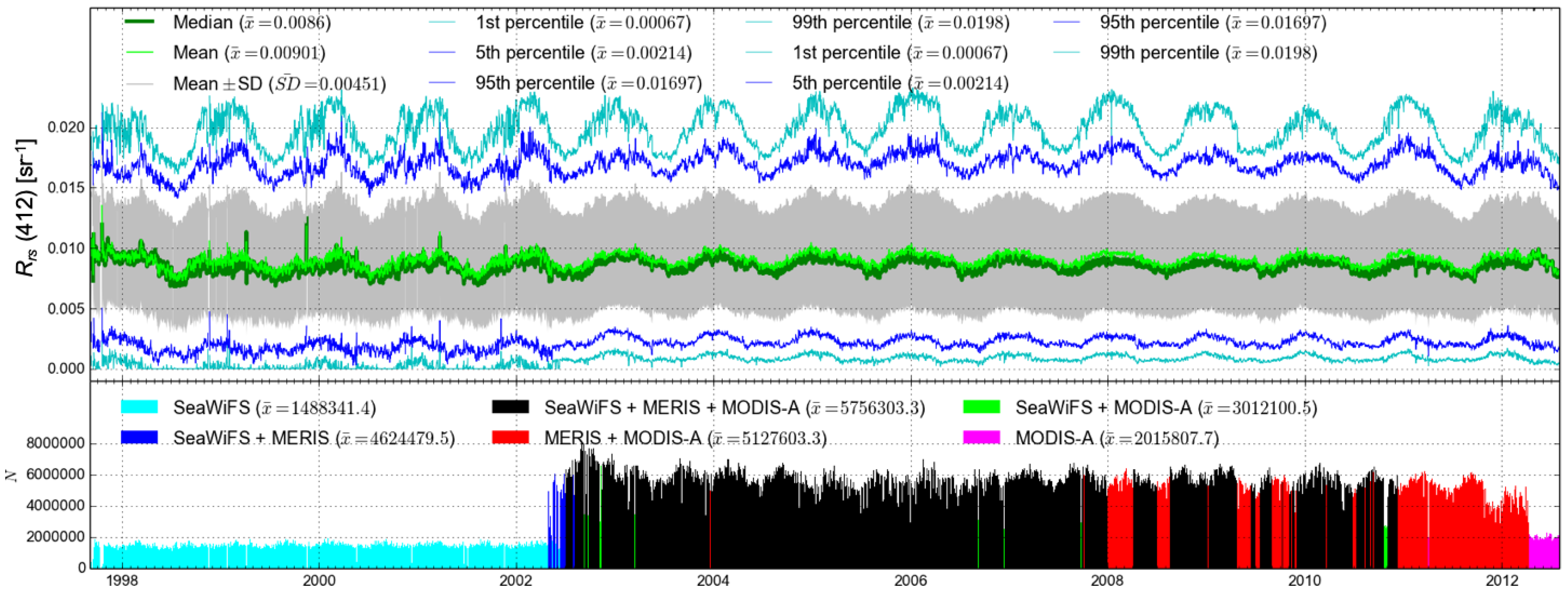
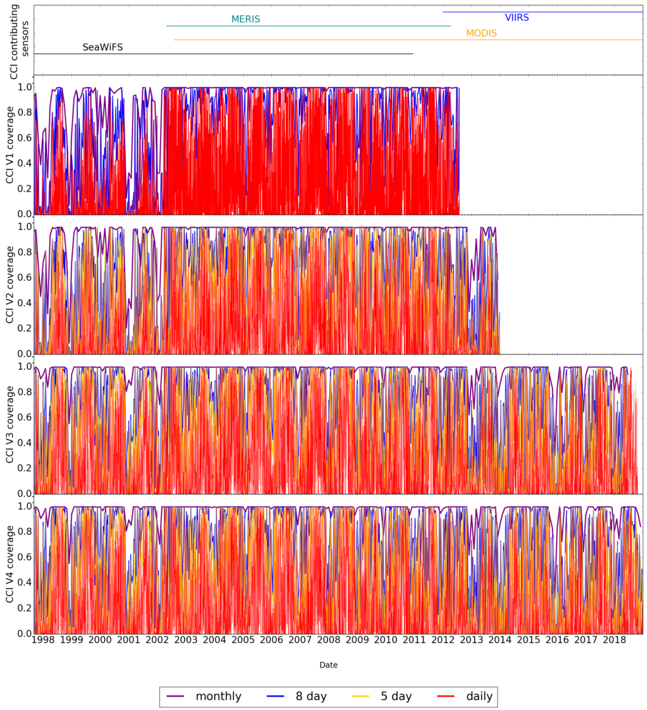
3.1. Satellite Data
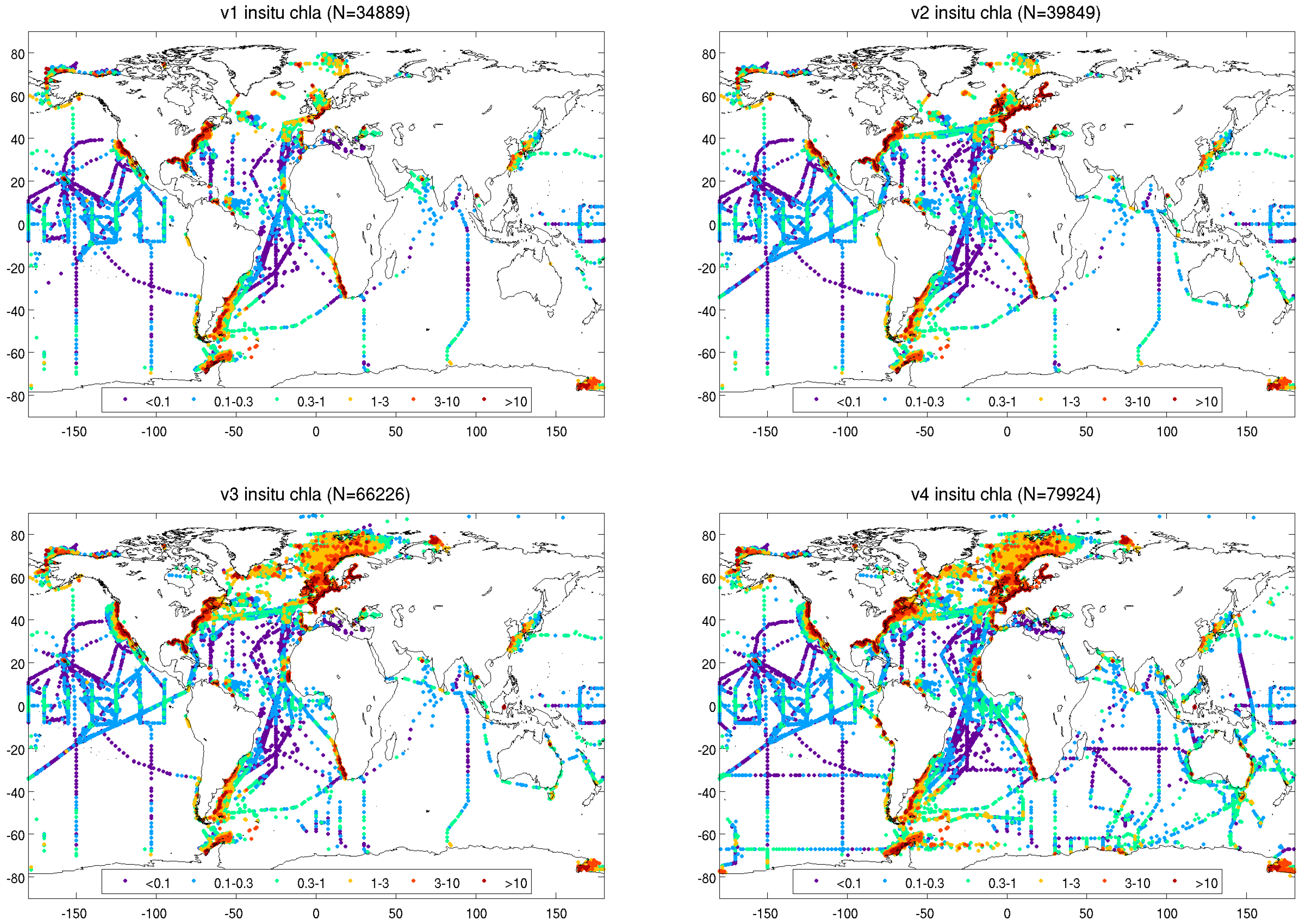
3.2. In Situ Data
3.3. Match-Up Database
4. Algorithm Selection Criteria
4.1. Objective Scoring System Based on Quantitative and Qualitative Criteria
4.1.1. Quantitative Criteria
4.1.2. Qualitative Criteria
5. Atmospheric Correction
6. Pixel Identification
6.1. Cloud Screening
6.2. Sea-Ice Detection
6.3. Mixed-Pixel Identification
6.4. Validation of Pixel-Identification Algorithm
6.5. Additional Filters and Post-Filters
7. Band Shifting
8. Bias Correction and Merging
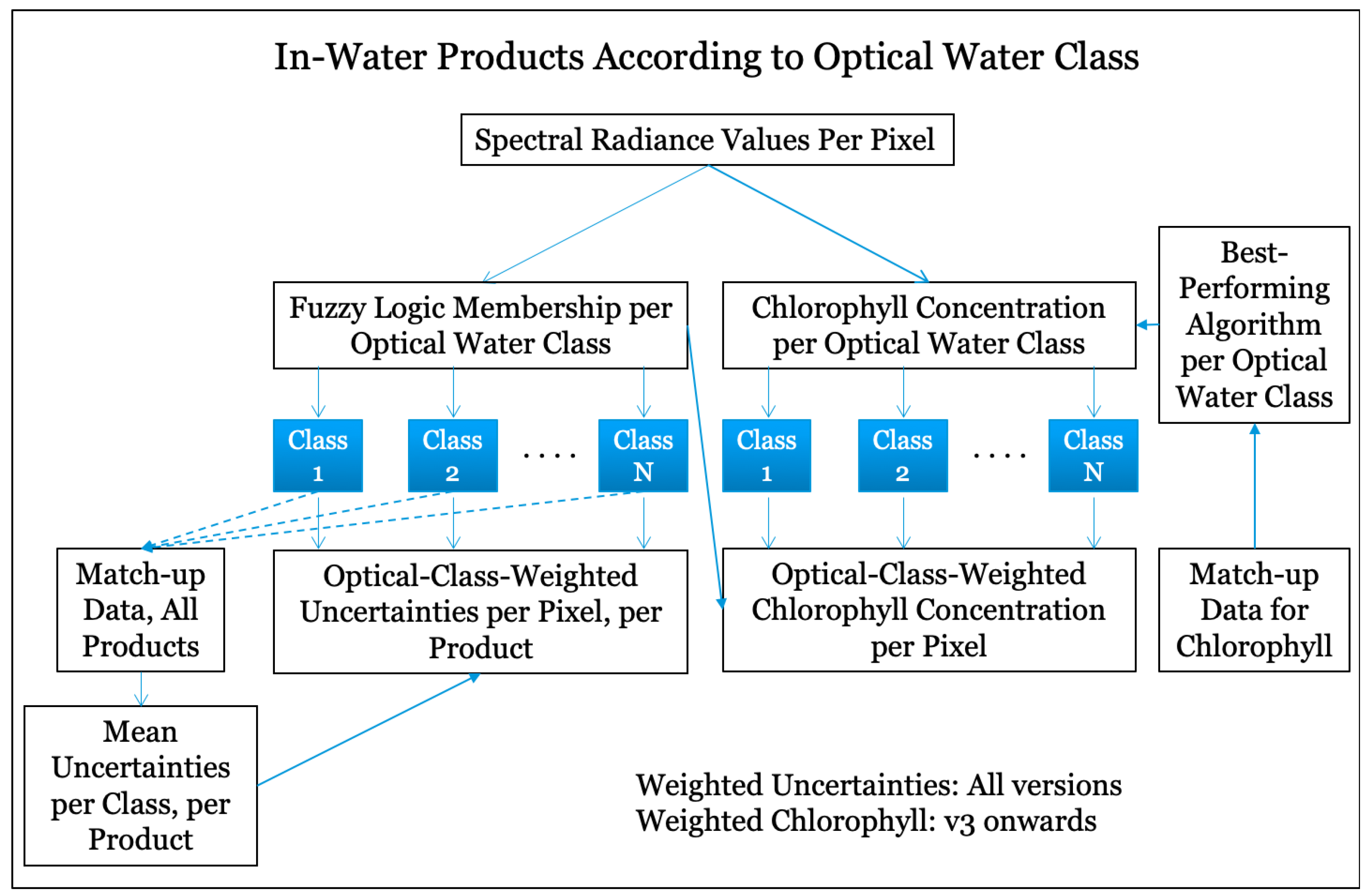
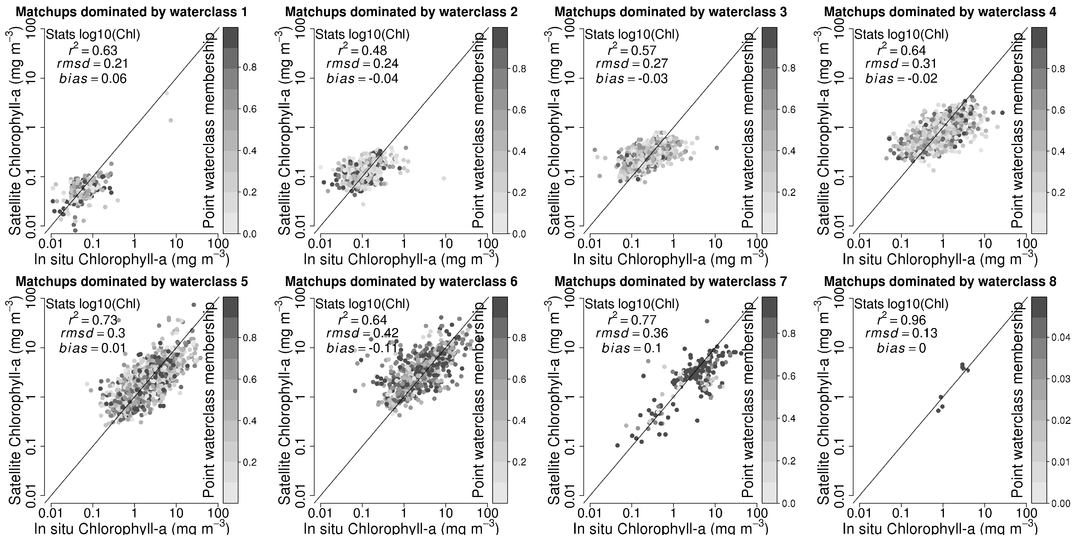
9. Generation of Optical Classes
10. In-Water Algorithms
11. Uncertainties: Root Mean Square Differences, Bias, and Relative Error
12. Product Generation
13. Validation of Products
14. Novel Features of the OC-CCI Time Series
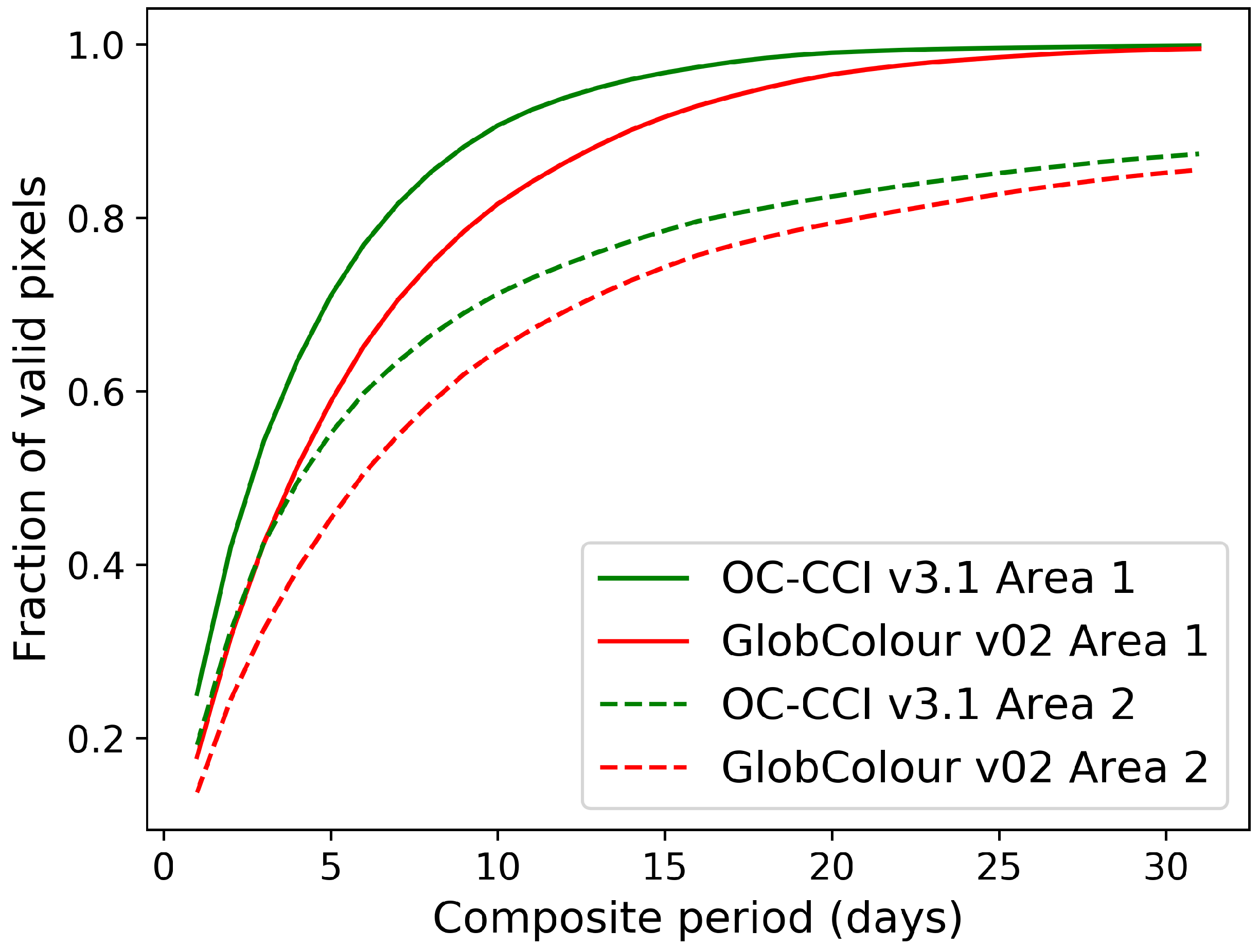
14.1. Improved Coverage
14.2. Uncertainty Characterisation Based on Validation
14.3. Merged Radiances that Band Shifted and Bias Corrected
15. Concluding Remarks
Supplementary Materials
Author Contributions
Funding
Acknowledgments
Conflicts of Interest
References
- Platt, T.; Hoepffner, N.; Stuart, V.; Brown, C. (Eds.) Why Ocean Colour? The Societal Benefits of Ocean-Colour Technology; Reports of the International Ocean Colour Coordinating Group; IOCCG: Dartmouth, NS, Canada, 2008; Volume No. 7. [Google Scholar]
- Longhurst, A.R.; Sathyendranath, S.; Platt, T.; Caverhill, C.M. An estimate of global primary production in the ocean from satellite radiometer data. J. Plankton Res. 1995, 17, 1245–1271. [Google Scholar] [CrossRef]
- Le Quéré, C.; Harrison, S.P.; Colin Prentice, I.; Buitenhuis, E.T.; Aumont, O.; Bopp, L.; Claustre, H.; Cotrim Da Cunha, L.; Geider, R.; Giraud, X.; et al. Ecosystem dynamics based on plankton functional types for global ocean biogeochemistry models. Glob. Chang. Biol. 2005, 11, 2016–2040. [Google Scholar] [CrossRef]
- Meskhidze, N.; Nenes, A. Effects of ocean ecosystem on marine aerosol-cloud interaction. Adv. Meteorol. 2010, 2010, 239808. [Google Scholar] [CrossRef]
- Krüger, O.; Graßl, H. Southern Ocean phytoplankton increases cloud albedo and reduced precipitation. Geophys. Res. Lett. 2011, 38, L08809. [Google Scholar] [CrossRef]
- Quinn, P.K.; Bates, T.S. The case against climate regulation via oceanic phytoplankton sulphur emissions. Nature 2005, 480, 51–56. [Google Scholar] [CrossRef]
- Shafeeque, M.; Sathyendranath, S.; George, G.; Balchand, A.; Platt, T. Seasonal cycle of phytoplankton off Somalia: Relationships to aerosols, winds and sea-surface temperature. Front. Mar. Sci. 2017, 4. [Google Scholar] [CrossRef]
- Muller-Karger, F.E.; Kavanaugh, M.; Montes, E.; Balch, W.; Breitbart, M.; Chavez, F.; Doney, S.; Johns, E.; Letelier, R.; Lomas, M.; et al. A framework for a marine biodiversity observing network within changing continental shelf seascapes. Oceanography 2014, 27, 18–23. [Google Scholar] [CrossRef][Green Version]
- Sathyendranath, S.; Gouveia, A.D.; Shetye, S.R.; Ravindran, P.; Platt, T. Biological control of surface temperature in the Arabian Sea. Nature 1991, 349, 54–56. [Google Scholar] [CrossRef]
- Wu, Y.; Tang, C.C.L.; Sathyendranath, S.; Platt, T. The impact of bio-optical heating on the properties of the upper ocean: A sensitivity study using a 3-D circulation model for the Labrador Sea. Deep-Sea Res. 2007, 54, 2630–2642. [Google Scholar] [CrossRef]
- Zhai, L.; Tang, C.; Platt, T.; Sathyendranath, S. Ocean response to attenuation of visible light by phytoplankton in the Gulf of St. Lawrence. J. Mar. Syst. 2011, 88, 285–297. [Google Scholar] [CrossRef]
- GCOS. Systematic Observation Requirements from Satellite-Based Data Products for Climate 2011 Update. Supplemental Details to the Satellite-Based Component of the “Implementation Plan for the Global Observing System for Climate in Support of the UNFCCC”; Technical Report, No. 154; World Meteorological Organisation (WMO): Geneva, Switzerland, 2011. [Google Scholar]
- GCOS. GCOS 2016 Implementation Plan; Technical Report; World Meteorological Organization: Geneva, Switzerland, 2016. [Google Scholar]
- Trenberth, K.E.; Hurrell, J.W. Decadal atmosphere-ocean variations in the Pacific. Clim. Dyn. 1994, 9, 303–319. [Google Scholar] [CrossRef]
- Schlesinger, M.E.; Ramankutty, N. An oscillation in the global climate system of period 65–70 years. Nature 1994, 367, 723–726. [Google Scholar] [CrossRef]
- Henson, S.A.; Sarmiento, J.L.; Dunne, J.P.; Bopp, L.; Lima, I.; Doney, S.C.; John, J.; Beaulieu, C. Detection of anthropogenic climate change in satellite records of ocean chlorophyll and productivity. Biogeosciences 2010, 7, 621–640. [Google Scholar] [CrossRef]
- Plummer, S.; Lecomte, P.; Doherty, M. The ESA Climate Change Initiative (CCI): A European contribution to the generation of the Global Climate Observing System. Remote Sens. Environ. 2017, 203, 2–8. [Google Scholar] [CrossRef]
- Steinmetz, F.; Deschamps, P.Y.; Ramon, D. Atmospheric correction in presence of sun glint: Application to MERIS. Opt. Express 2011, 19, 9783–9800. [Google Scholar] [CrossRef] [PubMed]
- Lee, Z.; Carder, K.L.; Arnone, R.A. Deriving inherent optical properties from water color: A multiband quasi-analytical algorithm for optically deep waters. Appl. Opt. 2002, 41, 5755–5772. [Google Scholar] [CrossRef]
- Sathyendranath, S. User Requirements Document, D 1.1, Ocean Colour Climate Change Initiative—Phase One. Version 1.11; Technical Report; European Space Agency: Paris, France, 2011. [Google Scholar]
- Sathyendranath, S.; Brewin, R.J.W.; Jackson, T.; Mélin, F.; Platt, T. Ocean-colour products for climate-change studies: What are their ideal characteristics? Remote Sens. Environ. 2017, 203, 125–138. [Google Scholar] [CrossRef]
- Valente, A.; Sathyendranath, S.; Brotas, V.; Groom, S.; Grant, M.; Taberner, M.; Antoine, D.; Arnone, R.; Balch, W.M.; Barker, K.; et al. A compilation of global bio-optical in situ data for ocean-colour satellite applications. Earth Syst. Sci. Data 2016, 8, 235–252. [Google Scholar] [CrossRef]
- Valente, A.; Sathyendranath, S.; Brotas, V.; Groom, S.; Grant, M.; Taberner, M.; Antoine, D.; Arnone, R.; Balch, W.M.; Barker, K.; et al. A compilation of global bio-optical in situ data for ocean-colour satellite applications—Version two. Earth Syst. Sci. Data Discuss. 2019, 2019, 1–54. [Google Scholar] [CrossRef]
- Sathyendranath, S.; Groom, S.; Grant, M.; Brewin, R.; Thompson, A.; Chuprin, A.; Horseman, A.; Jackson, T.; Martinez Vicente, V.; Platt, T.; et al. ESA Ocean Colour Climate Change Initiative (Ocean_Colour_cci): Version 1.0 Data; Technical Report; Centre for Environmental Data Analysis: Harwell, UK, 2016. [Google Scholar] [CrossRef]
- Sathyendranath, S.; Groom, S.; Grant, M.; Brewin, R.; Thompson, A.; Chuprin, A.; Horseman, A.; Jackson, T.; Martinez Vicente, V.; Platt, T.; et al. ESA Ocean Colour Climate Change Initiative (Ocean_Colour_cci): Version 2.0 Data; Technical Report; Centre for Environmental Data Analysis: Harwell, UK, 2016. [Google Scholar] [CrossRef]
- Sathyendranath, S.; Grant, M.; Brewin, R.J.W.; Brockmann, C.; Brotas, V.; Chuprin, A.; Doerffer, R.; Dowell, M.; Farman, A.; Groom, S.; et al. ESA Ocean Colour Climate Change Initiative (Ocean_Colour_cci): Version 3.1 Data; Technical Report; Centre for Environmental Data Analysis: Harwell, UK, 2018. [Google Scholar] [CrossRef]
- Sathyendranath, S.; Jackson, T.; Brockmann, C.; Brotas, V.; Calton, B.; Chuprin, A.; Clements, O.; Cipollini, P.; Danne, O.; Dingle, J.; et al. ESA Ocean Colour Climate Change Initiative (Ocean_Colour_cci): Version 4.0 Data; Technical Report; Centre for Environmental Data Analysis: Harwell, UK; Available online: http://catalogue.ceda.ac.uk/uuid/00b5fc99f9384782976a4453b0148f49.
- Morel, A.; Gentilli, B. Diffuse Reflectance of Oceanic Waters. 3. Implications of Bidirectionality for the Remote-Sensing Problem. Appl. Opt. 1996, 35, 4850–4862. [Google Scholar] [CrossRef]
- Morel, A.; Antoine, D.; Gentili, B. Bidirectional reflectance of oceanic waters: Accounting for Raman emission and varying particle scattering phase function. Appl. Opt. 2002, 41, 6289–6306. [Google Scholar] [CrossRef] [PubMed]
- Gordon, H.R.; Clark, D.K. Remote sensing of optical properties of a stratified ocean: An improved interpretation. Appl. Opt. 1980, 19, 3428–3430. [Google Scholar] [CrossRef] [PubMed]
- Sathyendranath, S.; Platt, T. Remote sensing of ocean chlorophyll: Consequence of non-uniform pigment profile. Appl. Opt. 1989, 28, 490–495. [Google Scholar] [CrossRef] [PubMed]
- Zaneveld, J.R.V.; Barnard, A.H.; Boss, E. Theoretical derivation of the depth average of remotely sensed optical parameters. Opt. Express 2005, 13, 9052–9061. [Google Scholar] [CrossRef] [PubMed]
- Brewin, R.J.W.; Sathyendranath, S.; Müller, D.; Brockmann, C.; Deschamps, P.Y.; Devred, E.; Doerffer, R.; Fomferra, N.; Franz, B.; Grant, M.; et al. The Ocean Colour Climate Change Initiative: III. A round-robin comparison on in-water bio-optical algorithms. Remote Sens. Environ. 2015, 162, 271–294. [Google Scholar] [CrossRef]
- Müller, D.; Krasemann, H.; Brewin, R.; Brockmann, C.; Deschamps, P.Y.; Doerffer, R.; Fomferra, N.; Franz, B.; Grant, M.G.; Groom, S.B.; et al. The Ocean Colour Climate Change Initiative: I. An Assessment of Atmospheric Correction Processors based on in-situ measurements. Remote Sens. Environ. 2014, 162, 242–256. [Google Scholar] [CrossRef]
- Müller, D.; Krasemann, H.; Brewin, R.; Brockmann, C.; Deschamps, P.Y.; Doerffer, R.; Fomferra, N.; Franz, B.; Grant, M.G.; Groom, S.B.; et al. The Ocean Colour Climate Change Initiative: II. Spatial and Seasonal Homogeneity of Atmospheric Correction Algorithms. Remote Sens. Environ. 2015, 162, 257–270. [Google Scholar] [CrossRef]
- Efron, B. Bootstrap methods: Another look at the jackknife. Ann. Stat. 1979, 7, 1–26. [Google Scholar] [CrossRef]
- Efron, B.; Tibshirani, R.J. An Introduction to the Bootstrap; Chapman and Hall: New York, NY, USA, 1993. [Google Scholar]
- Doney, S.C.; Lima, I.D.; Moore, J.K.; Lindsay, K.; Behrenfeld, M.J.; Westberry, T.K.; Mahowald, N.; Glover, D.M.; Takahashi, T. Skill metrics for confronting global upper ocean ecosystem-biogeochemistry models against field and remote sensing data. J. Mar. Syst. 2009, 76, 95–112. [Google Scholar] [CrossRef]
- Friedrichs, M.A.M.; Carr, M.E.; Barber, R.T.; Scardi, M.; Antoine, D.; Armstrong, R.A.; Asanuma, I.; Behrenfeld, M.; Buitenhuis, E.T.; Chai, F.; et al. Assessing the uncertainties of model estimates of primary productivity in the tropical Pacific Ocean. J. Mar. Syst. 2009, 76, 113–133. [Google Scholar] [CrossRef]
- Zibordi, G.; Mélin, F.; Voss, K.; Johnson, B.; Franz, B.; Kwiatkowska, E.; Huot, J.P.; Wang, M.; Antoine, D. System vicarious calibration for ocean color climate change applications: Requirements for in situ data. Remote Sens. Environ. 2015, 159, 361–369. [Google Scholar] [CrossRef]
- Gordon, H.R. In-orbit calibration strategy for ocean color sensors. Remote Sens. Environ. 1998, 63, 265–278. [Google Scholar] [CrossRef]
- Franz, B.A.; Bailey, S.W.; Werdell, P.J.; McClain, C.R. Sensor-independent approach to the vicarious calibration of satellite ocean color radiometry. Appl. Opt. 2007, 46, 5068–5082. [Google Scholar] [CrossRef] [PubMed]
- Clark, D.; Yarbrough, M.A.; Feinholz, M.E.; Flora, S.; Broenkow, W.; Kim, Y.S.; Johnson, B.C.; Brown, S.W.; Yuen, M.; Mueller, J.L. MOBY, a Radiometric Buoy for Performance Monitoring and Vicarious Calibration of Satellite Ocean Color Sensors: Measurement and Data Analysis Protocols; Technical Report, Ocean Optics Protocols for Satellite Ocean Color Sensor Validation, Revision 4, Volume VI: Special Topics in Ocean Optics Protocols and Appendices; (NASA/TM-2003-211621/Rev4-Vol.VI:3-34; Chapter 2); NASA Technical Reports Server (NTRS): Greenbelt, MD, USA, 2003. [Google Scholar]
- Mazeran, C.; Brockmann, C.; Ruescas, A.; Steinmetz, F.; Zühlke, M. A revisit of system vicarious calibration for non-standard ocean colour algorithm. Application to SeaWiFS, MODIS and MERIS data processed by POLYMER. Remote. Sens. Environ. in revision.
- North, P.; Brockmann, C.; Fischer, J.; Gomez-Chova, L.; Grey, W.; Heckel, A.; Moreno, J.; Preusker, R.; Regner, P. MERIS/AATSR synergy algorithms for cloud screening, aerosol retrieval and atmospheric correction. In Proceedings of the 2nd MERIS-AATSR User Workshop, Frascati, Italy, 22–26 September 2008. [Google Scholar]
- Gómez-Chova, L.; Camps-Valls, G.; Calpe-Maravilla, J.; Guanter, L.; Moreno, J. Cloud-screening algorithm for ENVISAT/MERIS multispectral images. IEEE Trans. Geosci. Remote Sens. 2007, 45, 4105–4118. [Google Scholar] [CrossRef]
- Kahru, M.; Elmgren, R. Multidecadal time series of satellite-detected accumulations of cyanobacteria in the Baltic Sea. Biogeosciences 2014, 11, 3619–3633. [Google Scholar] [CrossRef]
- Adams, J.; Smith, M.; Gillespie, A. Simple models for complex natural surfaces: A strategy for the hyperspectral era of remote sensing. In Proceedings of the 12th 1989 International Canadian Symposium on Remote Sensing Geoscience and Remote Sensing Symposium, Vancouver, BC, Canada, 10–14 July 1989; Volume 1, pp. 16–21. [Google Scholar] [CrossRef]
- Zibordi, G.; Holben, B.; Slutsker, I.; Giles, D.; D’Alimonte, D.; Mélin, F.; Berthon, J.F.; Vandemark, D.; Feng, H.; Schuster, G.; et al. AERONET-OC: A network for the validation of ocean color primary radiometric products. J. Atmos. Ocean. Technol. 2009, 26, 1634–1651. [Google Scholar] [CrossRef]
- Zibordi, G.; Mélin, F.; Berthon, J.F. Intra-annual variations of biases in remote sensing primary ocean color products at a coastal site. Remote Sens. Environ. 2012, 124, 627–636. [Google Scholar] [CrossRef]
- Antoine, D.; Guevel, P.; Desté, J.F.; Bécu, G.; Louis, F.; Scott, A.J.; Bardey, P. The “BOUSSOLE” Buoy—A new transparent-to-swell taut mooring dedicated to marine optics: Design, tests, and performance at sea. J. Atmos. Ocean. Technol. 2008, 25, 968–989. [Google Scholar] [CrossRef]
- Mélin, F.; Zibordi, G.; Berthon, J.F.; Bailey, S.; Franz, B.; Voss, K.; Flora, S.; Grant, M. Assessment of MERIS reflectance data as processed with SeaDAS over the European seas. Opt. Express 2011, 19, 25657–25671. [Google Scholar] [CrossRef]
- Mélin, F.; Sclep, G. Band shifting for ocean color multi-spectral reflectance data. Opt. Express 2015, 23, 2262–2279. [Google Scholar] [CrossRef] [PubMed]
- Bricaud, A.; Babin, M.; Morel, A.; Claustre, H. Variability in the chlorophyll specific absorption coefficients of natural phytoplankton: Analysis and parameterization. J. Geophys. Res. 1995, 100, 13321–13332. [Google Scholar] [CrossRef]
- Mélin, F.; Zibordi, G.; Berthon, J.F. Assessment of satellite ocean color products at a coastal site. Remote Sens. Environ. 2007, 110, 192–215. [Google Scholar] [CrossRef]
- Mélin, F.; Franz, B. Assessment of satellite radiometry in the visible domain. In Optical Radiometry for Oceans Climate Measurements; Donlon, C., Parr, A., Zibordi, G., Eds.; Elsevier Physical Science Series; Elsevier: Amsterdam, The Netherland, 2014; Chapter 6.1. [Google Scholar]
- Maritorena, S.; Siegel, D.A. Consistent merging of satellite ocean color data sets using a bio-optical model. Remote Sens. Environ. 2005, 94, 429–440. [Google Scholar] [CrossRef]
- Mélin, F.; Zibordi, G. Optically based technique for producing merged spectra of water-leaving radiances from ocean color remote sensing. Appl. Opt. 2007, 46, 3856–3869. [Google Scholar] [CrossRef]
- Mélin, F.; Zibordi, G.; Djavidnia, S. Merged series of normalized water leaving radiances obtained from multiple satellite missions for the Mediterranean Sea. Adv. Space Res. 2009, 43, 423–437. [Google Scholar] [CrossRef]
- Mélin, F.; Vantrepotte, V.; Clerici, M.; D’Alimonte, D.; Zibordi, G.; Berthon, J.F.; Canuti, E. Multi-sensor satellite time series of optical properties and chlorophyll-a concentration in the Adriatic Sea. Prog. Oceanogr. 2011, 91, 229–244. [Google Scholar] [CrossRef]
- Djavidnia, S.; Mélin, F.; Hoepffner, N. Comparison of global ocean colour data records. Ocean Sci. 2010, 6, 61–76. [Google Scholar] [CrossRef]
- Mélin, F. Global Distribution of the Random Uncertainty Associated with Satellite-Derived Chl A. IEEE Geosci. Remote Sens. Lett. 2010, 7, 220–224. [Google Scholar] [CrossRef]
- Mélin, F. Comparison of SeaWiFS and MODIS time series of inherent optical properties for the Adriatic Sea. Ocean Sci. 2011, 7, 351–361. [Google Scholar] [CrossRef]
- Moore, T.S.; Campbell, J.W.; Dowell, M.D. A class-based approach to characterizing and mapping the uncertainty of the MODIS ocean chlorophyll product. Remote Sens. Environ. 2009, 113, 2424–2430. [Google Scholar] [CrossRef]
- Moore, T.; Dowell, M.D.; Franz, B. Detection of coccolithophore blooms in ocean color satellite imagery: A generalized approach for use with multiple sensors. Remote Sens. Environ. 2012, 117, 249–263. [Google Scholar] [CrossRef]
- Jackson, T.; Sathyendranath, S.; Mélin, F. An improved optical classification scheme applied to ocean colour ECV. Remote Sens. Environ. 2017, 203, 152–161. [Google Scholar] [CrossRef]
- Lee, Z.; Lubac, B.; Werdell, P.J.; Arnone, R. An Update of the Quasi-Analytical Algorithm (QAA_v5). Technical Report, International Ocean Colour Coordinating Group (IOCCG). 2009. Available online: http://www.ioccg.org/groups/software.html (accessed on 10 February 2012).
- Lee, Z.; Du, K.; Arnone, R. A model for the diffuse attenuation coefficient of downwelling irradiance. J. Geophys. Res. 2005, 110, C02016. [Google Scholar] [CrossRef]
- Werdell, P.J.; Franz, B.A.; Bailey, S.W.; Feldman, G.C.; Boss, E.; Brando, V.E.; Dowell, M.; Hirata, T.; Lavender, S.J.; Lee, Z.; et al. Generalized ocean color inversion model for retrieving marine inherent optical properties. Appl. Opt. 2013, 52, 2019–2037. [Google Scholar] [CrossRef] [PubMed]
- Merchant, C.; Paul, F.; Popp, T.; Ablain, M.; Bontemps, S.; Defourny, P.; Hollmann, R.; Lavergne, T.; Laeng, A.; de Leeuw, G.; et al. Uncertainty information in climate data records from Earth observation. Earth Syst. Sci. Data 2017, 9, 511–527. [Google Scholar] [CrossRef]
- Fomferra, N.; Böttcher, M.; Zühlke, M.; Brockmann, C.; Kwiatkowska, E. Calvalus: Full-mission EO cal/val, processing and exploitation services. In Proceedings of the 2012 IEEE International Geoscience and Remote Sensing Symposium (IGARSS), Munich, Germany, 22–27 July 2012; pp. 5278–5281. [Google Scholar] [CrossRef]
- Maritorena, S.; Fanton d’Andon, O.H.; Mangin, A.; Siegel, D.A. Merged satellite ocean color data products using a bio-optical model: Characteristics, benefits and issues. Remote Sens. Environ. 2010, 114, 1791–1804. [Google Scholar] [CrossRef]
- Mélin, F. Ocean colour data bias correction and merging. In Algorithm Theoretical Basis Document, Ocean Colour Climate Change Initiative; Technical Report; ESA: Paris, France, 2014. [Google Scholar]
- Ciavatta, S.; Torres, R.; Saux-Picart, S.; Allen, I. Can ocean color assimilation improve biogeochemical hindcasts in shelf seas? J. Geophys. Res. 2011, 116. [Google Scholar] [CrossRef]
- Dutkiewicz, S.; Hickman, A.E.; Jahn, O.; Henson, S.; Beaulieu, C.; Monier, E. Ocean colour signature of climate change. Nat. Commun. 2019, 10. [Google Scholar] [CrossRef]


| Acronyms & Notations | Expansions & Definitions |
|---|---|
| bias correction | |
| wavelength | |
| median ratio | |
| absorption coefficient of detrital particles and coloured dissolved organic matter (or gelbstoff) combined | |
| absorption coefficient of phytoplankton | |
| total absorption coefficient | |
| back-scattering coefficient for particles | |
| vertical attenuation coefficient for downwelling irradiance | |
| normalised remote-sensing reflectance | |
| AOP | Apparent Optical Property |
| CCI | Climate Change Initiative |
| CF | Climate and Forecast |
| ECV | Essential Climate Variable |
| ESA | European Space Agency |
| GAC | Global Area Coverage |
| GCOS | Global Climate Observing System |
| HDFS | Hadoop Distributed File System |
| HPLC | High-Performance Liquid Chromatography |
| IOCCG | International Ocean Colour Coordinating Group |
| IOP | Inherent Optical Property |
| LAC | Local Area Coverage |
| L2Gen | NASA’s Level 2 Generator |
| MERIS | MEdium spectral Resolution Imaging Spectrometer |
| MERMAID | MERis MAtchup In Situ Database |
| MODIS-Aqua | Moderate-resolution Imaging Spectroradiometer-Aqua |
| NASA | National Aeronautics and Space Administration |
| NCEP | National Center for Environmental Prediction |
| NetCDF | Network Common Data Form |
| NOMAD | NASA bio-Optical Marine Algorithm Dataset |
| OC-CCI | Ocean-Colour Climate Change Initiative |
| OBPG | Ocean Biology Processing Group (of NASA) |
| PAR | Photosynthetically Available Radiation |
| POLYMER | POLYnomial based algorithm applied to MERIS |
| QAA | Quasi-Analytical Algorithm (QAA [19]) |
| SVC | System Vicarious Calibration |
| SWIR | Short-wave infrared |
| VIIRS | Visible and Infrared Imaging Radiometer Suite |
| Processing Step | Version 1 | Version 2 | Version 3.1 | Version 4 |
|---|---|---|---|---|
| Inputs | SeaWiFS GAC, MERIS, MODIS-A | SeaWiFS GAC, MERIS, MODIS-A | SeaWiFS GAC+LAC, MERIS, MODIS-A, VIIRS | SeaWiFS GAC+LAC, MERIS, MODIS-A, VIIRS |
| Input datasets | SeaWiFS: R2010.0; MODIS-A: R2013.1; MERIS: R3 | SeaWiFS: R2010.0; MODIS-A: R2013.1; MERIS: R3 | SeaWiFS: R2010.0; MODIS-A: R2014.0.1; MERIS: R3 | SeaWiFS: R2018; MODIS-A: R2018; VIIRS: R2018; MERIS: R3 |
| Atmospheric correction | POLYMER v2.7.0: MERIS; L2Gen 7.0: SeaWiFS, MODIS-A | POLYMER v3.0: MERIS;L2Gen: SeaWiFS, MODIS-A | POLYMER v3.5: MERIS, MODIS-A; L2Gen 7.3: SeaWiFS, VIIRS | POLYMER v4.8: MERIS;L2Gen v7.5: SeaWiFS, MODIS-A, VIIRS |
| in situ database | Initial version | Extended version with substantial increase in number of match-ups [22] | Further expanded in situ database | Further expanded in situ database [23] |
| Binning | Beam Binner: MERIS;L2Gen Binner: SeaWiFS, MODIS-A | Beam Binner v5 for all sensors, improving consistency; better binning algorithm | Further improvements in the binning algorithm to eliminate speckle | No change in binner from v3.1 |
| Bias correction | Static correction per pixel | Incorporates improved seasonal variation in bias | Incorporates weekly composites, giving smoother, fuller correction | No change in bias correction from v3.1 |
| Pixel identification | Idepix initial version: MERIS;L2Gen: SeaWiFS, MODIS-A | Idepix 2.0: SeaWiFS, MERIS;L2Gen: MODIS-A | Combination of Idepix and L2Gen | Combination of Idepix and L2Gen |
| Generation of optical classes | Used in situ database | Used OC-CCI v2 data | Used OC-CCI v3.1 data | Used OC-CCI v4 data |
| in situ algorithms | Best performing algorithms selected globally | Best performing algorithms selected globally | Best performing algorithms selected for each optical class | Best performing algorithms selected for each optical class |
| Uncertainty characterisation | Used v1 classes and initial in situ database | Used v2 classes and improved in situ v2 database | Used v3.1 classes and improved in situ database | Used v4 classes and improved in situ v4 database |
| Quality assurance | Initial version, less automated | More automated quality assurance process | More automated quality assurance process | More automated quality assurance process |
| Length of time series | September 1997 to December 2012 | September 1997 to December 2014 | September 1997 to December 2015 (extended to December 2018) | September 1997 to December 2018 |
| Doi: | 10.5285/E32FEB53-5DB1-44BC-8A09-A6275BA99407 | 10.5285/b0d6b9c5-14ba-499f-87c9-66416cd9a1dc | 10.5285/9c334fbe6d424a708cf3c4cf0c6a53f5 | 10.5285/00b5fc99f9384782976a4453b0148f49 |
| How to cite the data | Sathyendranath et al. 2016 [24] | Sathyendranath et al. 2016 [25] | Sathyendranath et al. 2018 [26] | Sathyendranath et al. 2019 [27] |
| PixBox Data | |||||
|---|---|---|---|---|---|
| Water | Cloud | Snow/Ice | |||
| IdePix data | water | 5433 | 23 | 2 | 5458 |
| cloud | 1033 | 15,068 | 2746 | 18,847 | |
| snow/ice | 2 | 66 | 1124 | 1192 | |
| 6468 | 15,157 | 3872 | 25,497 | ||
| Variable | v1 | v2 | v3.1 | v4 | |
|---|---|---|---|---|---|
| log(Chl-a) | RMSD | 0.303 | 0.328 | 0.314 | 0.340 |
| Bias | −0.0191 | −0.0284 | −0.00662 | −0.0409 | |
| 0.81 | 0.79 | 0.76 | 0.73 | ||
| N | 6049 | 7958 | 14,582 | 18,055 | |
| RMSD | 0.00128 | 0.00138 | 0.00130 | 0.00130 | |
| Bias | 8.68 | 2.60 | 3.94 | −7.44 | |
| 0.87 | 0.87 | 0.89 | 0.88 | ||
| N | 14,485 | 16,594 | 17,249 | 29,964 | |
| RMSD | 0.00114 | 0.00113 | 9.12 | 0.00111 | |
| Bias | −1.19 | −1.35 | 8.21 | −9.36 | |
| 0.83 | 0.81 | 0.86 | 0.83 | ||
| N | 12,711 | 19,128 | 18,614 | 32,186 | |
| RMSD | 0.00125 | 0.00101 | 0.00111 | 0.00106 | |
| Bias | 3.59 | 2.91 | 4.60 | 2.61 | |
| 0.76 | 0.77 | 0.79 | 0.79 | ||
| N | 15,112 | 21,346 | 21,794 | 34,546 | |
| RMSD | 0.000934 | 0.000658 | 0.000557 | 0.000678 | |
| Bias | 1.12 | 2.45 | 2.49 | 2.24 | |
| 0.54 | 0.45 | 0.36 | 0.47 | ||
| N | 3272 | 14,100 | 13,332 | 17,441 | |
| RMSD | 0.00155 | 0.00107 | 0.00132 | 0.00105 | |
| Bias | 6.23 | 3.04 | 5.30 | 2.73 | |
| 0.76 | 0.84 | 0.87 | 0.85 | ||
| N | 7490 | 14,862 | 15,194 | 17,557 | |
| RMSD | 0.000556 | 0.000401 | 0.000435 | 0.000473 | |
| Bias | −2.49 | 7.62 | 1.43 | 1.11 | |
| 0.68 | 0.77 | 0.80 | 0.78 | ||
| N | 5950 | 9429 | 9764 | 18,439 |
© 2019 by the authors. Licensee MDPI, Basel, Switzerland. This article is an open access article distributed under the terms and conditions of the Creative Commons Attribution (CC BY) license (http://creativecommons.org/licenses/by/4.0/).
Share and Cite
Sathyendranath, S.; Brewin, R.J.W.; Brockmann, C.; Brotas, V.; Calton, B.; Chuprin, A.; Cipollini, P.; Couto, A.B.; Dingle, J.; Doerffer, R.; et al. An Ocean-Colour Time Series for Use in Climate Studies: The Experience of the Ocean-Colour Climate Change Initiative (OC-CCI). Sensors 2019, 19, 4285. https://doi.org/10.3390/s19194285
Sathyendranath S, Brewin RJW, Brockmann C, Brotas V, Calton B, Chuprin A, Cipollini P, Couto AB, Dingle J, Doerffer R, et al. An Ocean-Colour Time Series for Use in Climate Studies: The Experience of the Ocean-Colour Climate Change Initiative (OC-CCI). Sensors. 2019; 19(19):4285. https://doi.org/10.3390/s19194285
Chicago/Turabian StyleSathyendranath, Shubha, Robert J.W. Brewin, Carsten Brockmann, Vanda Brotas, Ben Calton, Andrei Chuprin, Paolo Cipollini, André B. Couto, James Dingle, Roland Doerffer, and et al. 2019. "An Ocean-Colour Time Series for Use in Climate Studies: The Experience of the Ocean-Colour Climate Change Initiative (OC-CCI)" Sensors 19, no. 19: 4285. https://doi.org/10.3390/s19194285
APA StyleSathyendranath, S., Brewin, R. J. W., Brockmann, C., Brotas, V., Calton, B., Chuprin, A., Cipollini, P., Couto, A. B., Dingle, J., Doerffer, R., Donlon, C., Dowell, M., Farman, A., Grant, M., Groom, S., Horseman, A., Jackson, T., Krasemann, H., Lavender, S., ... Platt, T. (2019). An Ocean-Colour Time Series for Use in Climate Studies: The Experience of the Ocean-Colour Climate Change Initiative (OC-CCI). Sensors, 19(19), 4285. https://doi.org/10.3390/s19194285