Improved Remotely Sensed Total Basin Discharge and Its Seasonal Error Characterization in the Yangtze River Basin

Abstract

Total basin discharge is a critical component for the understanding of surface water exchange at the land–ocean interface. A continuous decline in the number of global hydrological stations over the past fifteen years has promoted the estimation of total basin discharge using remote sensing. Previous remotely sensed total basin discharge of the Yangtze River basin, expressed in terms of runoff, was estimated via the water balance equation, using a combination of remote sensing and modeled data products of various qualities. Nevertheless, the modeled data products are presented with large uncertainties and the seasonal error characteristics of the remotely sensed total basin discharge have rarely been investigated. In this study, we conducted total basin discharge estimation of the Yangtze River Basin, based purely on remotely sensed data. This estimation considered the period between January 2003 and December 2012 at a monthly temporal scale and was based on precipitation data collected from the Tropical Rainfall Measuring Mission (TRMM) satellite, evapotranspiration data collected from the Moderate Resolution Imaging Spectroradiometer (MODIS) satellite, and terrestrial water storage data collected from the Gravity Recovery and Climate Experiment (GRACE) satellite. A seasonal accuracy assessment was performed to detect poor performances and highlight any deficiencies in the modeled data products derived from the discharge estimation. Comparison of our estimated runoff results based purely on remotely sensed data, and the most accurate results of a previous study against the observed runoff revealed a Pearson correlation coefficient (PCC) of 0.89 and 0.74, and a root-mean-square error (RMSE) of 11.69 mm/month and 14.30 mm/month, respectively. We identified some deficiencies in capturing the maximum and the minimum of runoff rates during both summer and winter, due to an underestimation and overestimation of evapotranspiration, respectively.

1. Introduction

Total basin discharge (TBD) is a fundamental water balance component of river basins [1,2] and it has been traditionally measured at in-situ hydrological stations near estuary mouths. TBD can be converted into surface runoff (R) when considering a surface area unit over the entire river basin. Continuous TBD time series are necessary for the monitoring of hydrological extremes (i.e., droughts and floods) in deltaic regions. Such monitoring is important for better water management, allowing an increase in water usage efficiency and minimizing unpredictable human, agricultural, and economic losses [3,4,5,6,7]. Nevertheless, a comprehensive global river water discharge (RWD) observing network has not been established yet [8]; moreover, the number of in-situ stations has been decreasing since the late 1970s due to the absence of sufficient funding for the upgrade and maintenance of facilities [9,10]. Consequently, a gauge-independent method, which would provide a synoptic mean of observing the global RWD, remains elusive [11].

Remotely sensed RWD estimations based on the most recent (passive and active) remote sensing (RS) advances, have been demonstrated to be viable alternatives [12]. Over the long period, it is anticipated that remotely sensed RWD estimations will compensate the scarcity of in-situ hydrological data, particularly in remote regions. Current remotely sensed RWD methods can be classified into the following four categories:

(1)

The correlation between passive remotely sensed variables (e.g., Normalized Difference Vegetation Index (NDVI), and Land Surface Temperature (LST) [13,14,15,16]) and the water level (WL) or RWD data [17,18,19,20,21,22]. Notably, the above remotely sensed variables have no direct causal relationship with RWD.

(2)

The calculation of the RWD from passive remotely sensed hydraulic variables, via hydraulic geometric equations (e.g., [23,24,25,26,27,28,29]). In this case, the accuracy of RWD estimation would be region-dependent: the resolution of RS images might be insufficient to detect small changes in river width [30] and the roughness coefficient might be unavailable in some regions [31,32].

(3)

The correlation between active remotely sensed WL (collected from satellite radar altimetry) and in-situ RWD data (collected from hydrological stations) via stage–discharge rating curves [1,33,34,35]. In this case, the altimetry radar signals are partially contaminated by land surfaces when crossing rivers with short widths: the accuracy of the observed altimetric WL is limited (e.g., [36]).

(4)

The calculation of the RWD near the estuary mouth (or of R), based on the land water balance [37] or on the combined land–atmosphere water balance equation [38]. However, both observed and modeled data of various qualities have been utilized in previous studies based on this process (e.g., [39,40]).

The fourth method represents a purely hydrological modeling method that can be applied to the basin-wide estimation of R and does not rely on in-situ ground observations. This method involves the combined use of remotely sensed precipitation (P), terrestrial water storage (S), modeled evapotranspiration (ET) and/or modeled atmospheric moisture budget data (i.e., moisture flux divergence ($\nabla ·Q$), and the changes in the total column water vapor ($\frac{\partial W}{\partial t}$)). Both in the case of land-based (i.e., $R=P-ET-\Delta S$) [41,42] and combined land–atmosphere water balance (i.e., $R=-\Delta S-\frac{\partial W}{\partial t}-\nabla ·Q$) e.g., [43] equations, the quality of the modeled ET and of the atmospheric moisture budget results is limited by large uncertainties [44,45,46]. This is due to the fact that different land cover types and physical assumptions are considered for their calculation. Moreover, before the launch of Gravity Recovery and Climate Experiment (GRACE), the S values were unavailable and their change ($\Delta S$) was assumed to be zero [41,47]. This assumption caused further uncertainties in the estimation of the remotely sensed R.

The land–atmosphere water balance equation used for R estimation has been applied efficiently for the first time to the Amazon and Mississippi river basins [38]. The authors of that study used GRACE S and a modeled atmospheric moisture budget operational forecast analysis (provided by the Environmental Protection-National Center for Atmospheric Research (NCEP-NCAR) [48] and by the European Centre for Medium-Range Forecasts (ECMWF)). The estimated R for the Yangtze river basin (YRB) closely agrees with in-situ observed R: the peak-to-peak Pearson correlation coefficient (PCC) was equal to 0.92 [44]. Ferreira et al. (2013) [37] estimated R for the same river basin but based on the land-based water balance equation (using remotely sensed P from the Tropical Rainfall Measuring Mission (TRMM) [49], $\Delta S$ from GRACE [50], and modeled ET data from the Global Land Data Assimilation System (GLDAS) [45]). The result of Ferreira et al. (2013) [37] indicated a good agreement between the estimated R and the in-situ observed R time series (i.e., PCC 0.74 and root-mean-square error (RMSE) 14.30 mm/month).

The ET obtained from Moderate Resolution Imaging Spectroradiometer (MODIS) could conveniently replace the modeled ET, since the Penman–Monteith equation provided a better representation of croplands and grasslands [51]. These land cover types are densely situated within the YRB, particularly at the middle and lower reaches of the YRB. Previous accuracy assessment did not account for the potential existence of seasonal error characteristics and for deficiencies in the modeled data products (for the estimation of R). This study aims to address such issues; we applied a purely remotely sensed data-driven method based on the land water balance equation and able to estimate R in the YRB at a monthly temporal scale. This data-driven method is established using water balance equations in combination with TRMM P, MODIS ET, and GRACE $\Delta S$ data.

In China, food security relies on the water resources of the YRB; hence, this river basin is one of the most significant study areas [52]. A number of water management projects have been operated for adjustment of R during severe drought and flood seasons [53,54]. Other human activities, such as damming, groundwater withdrawal, water consumption, and land use change, can have substantial impacts on R of the river basin [55,56]. Land-use change accounts for <0.2% of the change in the runoff trend [57], while damming, groundwater withdrawal, and water consumption account for <2%, <1%, and <10% of the changes in the annual runoff [58], respectively. However, other research studies have indicated climate change as the main factor affecting R (accounting for 90% of the change in R in the YRB) [57,59,60,61]. Additional studies have indicated that human activities in the YRB might significantly influence changes in the sediments, but not in R [60,62].

Notably, the R values estimated from the water balance equation were calculated by subtraction among the remotely sensed P, ET, and ∆S: the systematic effect caused by the YRB environment and by human activities should have been partly mitigated by this subtraction process. The aforementioned information partially supports our data-driven R estimation for the YRB, based purely on the above remotely sensed hydrological variables on the application of the water balance equation. After calculating the resulting R, we compared our results with those published in Syed et al. (2009) [44] and Ferreira et al. (2013) [37]; moreover, we performed a seasonal accuracy assessment of the observed R time series, in order to evaluate the performance of our method during all seasons. Finally, we discussed the deficiencies of modeled data products and tried to explain the reasons for different seasonal discrepancies between the R obtained through our method and the observed in-situ data.

This paper is organized as follows: Section 2 presents the geographic environment of the YRB; Section 3 presents the methodology, data used in this study, and their validation; Section 4 demonstrates the validity of the estimated R and compares our results with those of previously published studies; and Section 5 summarizes our conclusions.

2. Geography of the Yangtze River Basin (YRB)

Situated between 25°–35° N and 91°–122° E, within the subtropical zone, the Yangtze River is the world’s third longest river and the first in China [63]. It flows from the three-rivers headwater region (northeastern Tibetan Plateau) to the East China Sea, for a total length of 6300 km and with a total drainage basin area of 1,800,000 km² [64,65]. The whole YRB (Figure 1) can be divided into three reaches, based on its stepped topography and on the river channel cross-sections: an upper (from the Tibetan Plateau to Yichang), a middle (from Yichang to Hukou), and a lower reach (from Hukou to the river estuary) [66].

The majority of the YRB is subject to the subtropical monsoons, in particular the Indian Summer Monsoon (ISM) and the East Asian Summer Monsoon (EASM) [67,68]. Generally, the surface air temperature in the YRB reaches maxima in summer and minima in winter [69]; moreover, P concentrates over the middle-lower reach of the YRB. The mean annual P rate in correspondence of the upper reach (i.e., 270–500 mm) is significantly lower than that in correspondence of the middle-lower reach (i.e., 1600–1900 mm) [70]. Controlled by the monsoonal climate, the rainy season starts from April and ends in September, peaking in July every year [71].

3. Methodology, Data Description and Validation

3.1. Methodology

The terrestrial water balance equation, based on the principle of mass conservation, has been used to estimate the remotely sensed runoff R for the YRB [41,42]:

$$R=P-ET-\Delta S$$

(1)

where P is the precipitation (mm/month), ET the evapotranspiration (mm/month), ∆S the terrestrial water storage change (mm/month), which can be expressed as:

$$\Delta S=\frac{1}{2}\left(S_{i+1}-S_{i-1}\right)$$

(2)

where $S_i$ is water storage anomaly (mm/month) of month i.

Table 1. Remotely sensed data products and in-situ gauge observations used in this study.

Hydrological Component	Data Source	Spatial Resolution	Temporal Resolution
Precipitation	TRMM 3B43 v7	$0.25°\times 0.25°$	Monthly
	Gauges	Point	Daily
Evapotranspiration	MOD16A2	$0.5°\times 0.5°$	Monthly
	GLDAS	$1°\times 1°$	Monthly
Evaporation	Gauges	Point	Daily
Terrestrial water storage change	GRACE	$3°\times 3°$	Monthly
	GLDAS	$1°\times 1°$	Monthly
Runoff	Gauges	Point	Daily

summarizes all the remotely sensed data products and the in-situ gauge observations used in this study. All the in-situ gauge data time series were obtained from the Changjiang Water Resources Commission (Ministry of Water Resources; http://www.cjh.com.cn). Notably, the remotely sensed P data from the TRMM, the ET data from the MODIS, and the S data from GRACE have different spatial resolutions (Table 1) and need to be unified. Therefore, the TRMM and MODIS data were resampled at a $1°\times 1°$ resolution, whereas the GRACE data were interpolated at a $1°\times 1°$ resolution. The remotely sensed data were then validated against the in-situ gauge at point locations. No in-situ ET gauge stations were available in the YRB [51]; hence, we needed to use the evaporation (E) in-situ measurements to infer the ET. Since terrestrial water storage measurements were unavailable at a point location, the GLDAS was employed to validate the data in this study.

Once the steps described above were completed, all the P, ET, and $\Delta S$ values gridded within the YRB up to Datong station location were individually summed up and used to calculate the monthly R values between 2003 and 2012 (see Equation (1) and Figure 1). To be comparable with the unit of the estimated R values, the daily observed discharge (${\mathrm{m}}^3/$sec) data of Datong station were combined to in the form of monthly discharge values and subsequently divided by the approximate total drainage area, up to Datong station (i.e., $1.7\times {10}^6{\mathrm{km}}^2$) to obtain the monthly R per unit area (mm/month) (Figure 1).

3.2. In-Situ Hydrological Gauge Stations as Reference Data

In proximity of the estuary mouth, the river channel is seasonally affected by a combination of fluvial (i.e., discharge) and marine (i.e., tide and wave) processes. The Datong station was chosen to validate the remotely sensed R (Figure 1), since it is sufficiently far from the estuary. For consistency with the RS data, we used the RWD time series collected at the Datong station between January 2003 and December 2012. The observed RWD data (m³/s) were converted into monthly R rates (mm/month) per unit area of the YRB. To validate the remotely sensed P (TRMM) and ET (MODIS) data, we considered the observed P and the inferred ET using Equation (6) of Zhang et al. (2001) [72] from the observed E data time series collected at stations along the upper (i.e., Pingshan), middle (i.e., Chenglingji), and lower reaches (i.e., Datong) of the Yangtze River (Figure 1).

The Datong station time series showed an annual peak and trough in July and February, respectively (Figure 2). The exceptionally large R that occurred in July 2010 was likely caused by a moderate El Niño event that started in autumn 2009, as also indicated by the Oceanic Niño Index (https://ggweather.com/enso/oni.htm).

3.3. Remotely Sensed Hydrological Variables and Their Validation

3.3.1. Evaluation Metrics

To estimate the remotely sensed R for the YRB, several remotely sensed datasets have been considered (i.e., P (TRMM), ET (MODIS), and S (GRACE) data). These datasets and the estimated R were subjected to an accuracy evaluation, by comparing them to the gauge station observed time series. In particular, the remotely sensed data were compared to the gauge station observed time series using the PCC and the RMSE, whereas the R values estimated from the water balance model were compared to the gauge station observed time series using the PCC, RMSE, and the Nash–Sutcliffe model efficiency (NSE) coefficient. The PCC is a number that represents the strength of the linear relationship between two data time series; it can be calculated as follows:

$$\mathrm{PCC}=\frac{{{\displaystyle \sum }}_{i=1}^N\left(X_o^i-\overline{X_o}\right)\left(X_m^i-\overline{X_m}\right)}{\sqrt{{{\displaystyle \sum }}_{i=1}^N{\left(X_o^i-\overline{X_o}\right)}^2}\sqrt{{{\displaystyle \sum }}_{i=1}^N{\left(X_m^i-\overline{X_m}\right)}^2}}$$

(3)

The RMSE represents the accuracy of the estimation; It can be calculated as follows:

$$\mathrm{RMSE}=\sqrt{\frac{{{\displaystyle \sum }}_{i=1}^N{\left(X_m^i-X_o^i\right)}^2}{N}}$$

(4)

The NSE coefficient proposed by Nash and Sutcliffe (1970) [73] is usually used to assess hydrological models; it can be calculated as follows:

$$\mathrm{NSE}=1-\frac{{{\displaystyle \sum }}_{i=1}^N{\left(X_m^i-X_o^i\right)}^2}{{{\displaystyle \sum }}_{i=1}^N{\left(X_o^i-\overline{X_o}\right)}^2}$$

(5)

where $X_o$ and $\overline{X_o}$ are the gauge observed and the average gauge observed values, respectively; $X_m$ and $\overline{X_m}$ represent the remotely sensed R and the average remotely sensed values, respectively; and N corresponds to the number of observations within the time series. The closer the NSE is to 1, the better the performance of $X_m$ is. Notably the numerical value of NSE should be equivalent to the coefficient of determination (R²), a statistical measure used to predict future outcomes and test hypotheses.

3.3.2. Remotely Sensed Precipitation

The Tropical Rainfall Measuring Mission (TRMM) is a satellite mission responsible for the spatiotemporal measurement of P over a large latitude interval (between 50° S and 50° N [74]). The monthly gridded global P data (TRMM3B43 V7) used in this study, having a spatial resolution of 0.25° [50], were obtained from the Goddard Earth Sciences Data and Information Services Center (GES DISC) managed by NASA (https://disc.gsfc.nasa.gov/datasets/TRMM_3B43_V7/summary downloaded on 14 June 2018). Notably the TRMM 3B43 V7 data products are not purely a satellite-based; in fact, the Global Precipitation Climatology Centre (GPCC) gauge data were used for bias correction and calibration [75,76,77].

Three hydrological stations were selected in the YRB and considered for the comparison between the satellite P (TRMM) and the observed monthly P data. The result showed that the satellite P (TRMM) and the observed P data were strongly correlated with each other in the case of all three stations, their the PCCs were equal to 0.82 (Pingshan station), 0.95 (Chenglingji station), and 0.88 (Datong station), respectively (

Table 2. Statistical comparison between the remotely sensed precipitation data and the observed precipitation data at the three selected stations, located along the upper, middle, and lower reaches of the Yangtze River basin.

Station	PCC	RMSE (mm/month)
Pingshan	0.82	50.8
Chenglingji	0.95	32.1
Datong	0.88	52.3

). Moreover, their respective RMSE values indicated similar conditions along the upper, middle, and lower river reaches, although the highest correlation was identified in correspondence of the middle reaches. Overall, the TRMM and observed P data series of the YRB were in good agreement with each other; hence, they were considered reliable for our study (Figure 3).

3.3.3. Remotely Sensed Evapotranspiration

Evapotranspiration (ET) is a water vapor that re-enters the atmosphere. It includes the evaporation from soil moisture and the transpiration from land vegetation [78]. The MOD16A2 ET data product was prepared based on the MODIS and Global Meteorological Assimilation Office (GMAO) data products using the Penman–Monteith equation [79], having the spatial coverage of 80° N–60° S and 0° E–360° E. These data products were obtained from the MODIS Global Evaporation Project (i.e., MOD16A2) dataset, managed by the Land Processes Distributed Active Archive Center (LP DAAC) of NASA (https://lpdaac.usgs.gov/dataset_discovery/modis/modis_products_table). These data products were also available at the Numerical Terradynamic Simulation Group in the University of Montana (http://www.ntsg.umt.edu/project/modis/).

Some controversy exists regarding the uncertainty of regional or global-scale ET [80,81]. Therefore, it was necessary to compare the MODIS ET data to the inferred ET using Equation (6) of Zhang et al. (2001) [72] from the observed E data. The results of this comparison showed that the MODIS ET were strongly correlated with the inferred ET along the middle and lower river reaches: the PCCs of 0.87 (Pingshan station), 0.71 (Chenglingji station), and 0.80 (Datong station), respectively (

Table 3. Statistical comparison between the remotely sensed MODIS evapotranspiration data and the inferred evapotranspiration from the observed evaporation data at the three selected stations along the upper, middle, and lower reaches of the Yangtze River basin.

Station	PCC	RMSE (mm/month)
Pingshan	0.87	26.4
Chenglingji	0.71	29.7
Datong	0.80	29.4

). Meanwhile, the respective magnitude of the RMSE values was apparently dependent on the amount of ET (Figure 4).

The MODIS ET data were also compared to the ET modeled data (derived from the GLDAS). Four different land surface models (i.e., the common land model (CLM), the Mosaic, the National centers for environmental prediction/Oregon State University/Air force/Hydrologic research lab (NOAH), and the variable infiltration capacity (VIC) model) were extracted. The MODIS ET and the four sets of GLDAS modeled data were characterized by strong and consistent PCCs; however, the RMSE values revealed diverse performances (

Table 4. Statistical comparison between remotely sensed MODIS evapotranspiration and the GLDAS modeled evapotranspiration data at the three selected stations along the upper, middle, and lower reaches of the Yangtze River basin.

Station	GLDAS	PCC	RMSE (mm/month)
Pingshan	CLM	0.94	16.5
	Mosaic	0.89	25.1
	Noah	0.95	19.6
	VIC	0.91	23.3
Chenglingji	CLM	0.92	14.5
	Mosaic	0.93	39.1
	Noah	0.94	29.4
	VIC	0.95	34.0
Datong	CLM	0.96	10.4
	Mosaic	0.91	30.0
	Noah	0.89	22.2
	VIC	0.95	25.5

). These results can be attributed to a consistency in the seasonal patterns, combined with a considerable variation in the occurrence of maxima during the summer season (Figure 5). For the entire YRB, the CLM ET data showed the best match with the MODIS ET data.

3.3.4. Remotely Sensed Terrestrial Water Storage

GRACE is a satellite mission responsible for measuring Earth’s time-variable gravity changes, which allow inference of global S variations (in terms of Equivalent Water Height (EWH)). The EWH were computed by the Center for Space Research (CSR), GeoForschungsZentrum (GFZ), the Institute of Theoretical geodesy and Satellite Geodesy (ITSG), and the Jet Propulsion Laboratory (JPL) GRACE Level-2 Release 05 (RL05) GSM monthly gravity fields for the period between January 2003 and December 2012 in the form of spherical harmonic coefficients (SHCs) [82].

Unified postprocessing procedures were applied to the SHCs before converting them into S data. The degree-one terms were restored to correct for the geocenter motion [83], while the term $C_{20}$ in the form of the SHCs was replaced by the Satellite Laser Ranging (SLR) results [84]. A destriping process and a Gaussian filtering (radius 350 km) were applied in order to reduce the spatially correlated errors of the S [85,86]. Afterward, the values of S time series were calculated considering a regular grid using Equation (14) in [87] and dividing the result by water density. Additionally, the sum of the preceding and succeeding two-month data were averaged in order to compensate for (i.e., interpolating) the missing monthly S data.

There is controversy about the uncertainty of the GLDAS-modeled S data, especially when compared to remotely sensed GRACE S data (e.g., [88]). Hence, the GRACE S data needed to be validated by comparing them with the GLDAS-modeled S data. Only the GRACE S data obtained from the CSR are shown in

Table 5. Statistical comparison between the remotely sensed GRACE (CSR) and the GLDAS-modeled terrestrial water storage datasets at the three selected stations along the upper, middle, and lower reaches of the Yangtze River basin.

	GLDAS	PCC	RMSE (mm/month)
Pingshan	CLM	0.03	49.09
	Mosaic	0.05	129.50
	Noah	0.38	66.40
	VIC	0.32	75.66
Chenglingji	CLM	0.43	56.93
	Mosaic	0.57	115.04
	Noah	0.52	68.12
	VIC	0.44	84.11
Datong	CLM	0.29	34.17
	Mosaic	0.56	91.10
	Noah	0.56	34.20
	VIC	0.41	60.31

, since all GRACE data products exhibited similar patterns (independently from the position of the correspondent stations). We noted a large disparity and a low correlation between the GRACE and the GLDAS-modeled S data (Table 5), particularly in correspondence of the river upper reaches. Moreover, the GLDAS-modeled S data series obtained from different sources were considerably different among each other (Figure 6). In fact, while the modeled CLM S data displayed small variability, those from Mosaic displayed large fluctuations. The modeled S data from the VIC and the NOAH showed modest fluctuation patterns, similar to that of the GRACE data. Furthermore, leakage errors in the GRACE S data and the uncertainties inherent to the GLDAS modeled S data could have contributed to their poor correlation (e.g., [89]). Therefore, it is difficult to assess the accuracy of the GRACE S simply based on the GLDAS modeled S data: the pure remotely sensed R and modeled (i.e., ET and/or S) datasets need to be further compared with each other.

4. Discussion

The resulting R time series based on our purely satellite data-driven method (i.e., MODIS ET and several GRACE S) were compared to remotely sensed and modeled data products (i.e., ITSG GRACE S and several GLDAS ET, or MODIS ET and several GLDAS S), which were based on the same TRMM P data (

Table 6. Statistical comparison between the remotely sensed monthly runoff data derived from the MODIS evapotranspiration and several GRACE terrestrial water storage, several GLDAS evapotranspiration and ITSG GRACE water storage, and MODIS evapotranspiration and several GLDAS terrestrial water storage data, and the ground-based observed runoff.

Dataset Combinations	PCC	RMSE(mm/month)	NSE
MODIS + JPL	0.88	11.89	0.631
MODIS + ITSG	0.89	11.69	0.643
MODIS + GFZ	0.88	11.78	0.638
MODIS + CSR	0.88	11.90	0.630
ITSG GRACE + CLM	0.73	15.69	0.357
ITSG GRACE + Mosaic	0.48	29.26	−1.235
ITSG GRACE + Noah	0.67	20.66	−1.146
ITSG GRACE + VIC	0.39	26.29	−0.805
MODIS + CLM	0.70	24.96	−0.627
MODIS + Mosaic	0.76	19.16	0.004
MODIS + Noah	0.76	20.82	−0.132
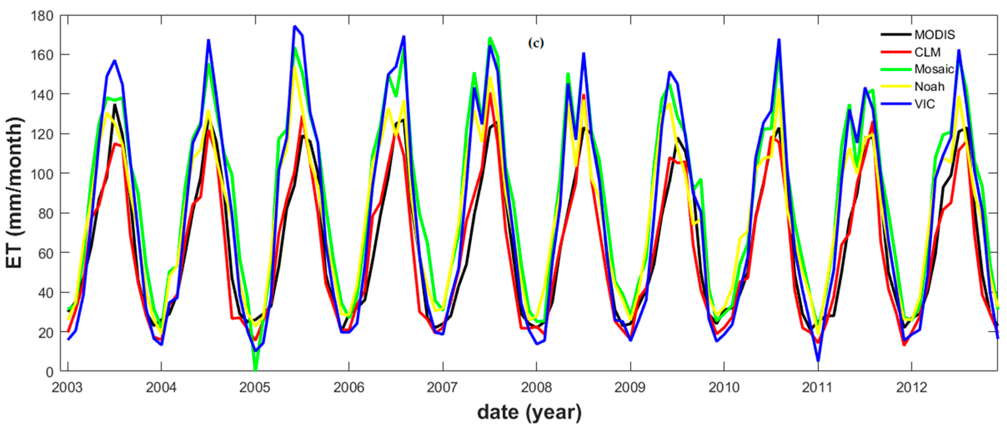
MODIS + VIC	0.76	21.41	−0.196

). Our analysis showed that the MODIS and ITSG, ITSG and CLM, and MODIS and Mosaic were the best data combinations to describe the remotely sensed ET and S changes (Figure 7). The combination (i.e., ITSG GRACE S and CLM ET) yields a PCC of 0.73 and an RMSE of 15.69 mm/month, comparable to those reported by Ferreira et al. (2013) [37] (i.e., 0.74 and 14.30 mm/month, respectively). Our metrics were slightly less accurate than those in [37], probably due to the additional three-year time span (between 2010 and 2012) considered in the study: during this period, the occurrence of a moderately strong El Niño event might have created anomalous conditions. In the case of the MODIS ET and GRACE S data, our data-driven method resulted in a PCC of 0.88 and an RMSE of 11.69 mm/month, indicating a higher accuracy than that obtained in [37]. According to the results, the MODIS16A2 ET data are more reliable than those of the GLDAS, at least for the YRB. Probably, this was due to the use of the Penman–Monteith equation during the production of the MODIS16A2 ET data: this equation favors the detection of cropland and grassland covers [51], particularly in the YRB.

Our results were validated against those result of Syed et al. (2009) [44] by considering the peak-to-peak correlation between the remotely sensed and the observed R (

Table 7. Peak-to-peak correlation between the remotely sensed runoff and the ground-based observed runoff.

Peak to Peak Correlation
MODIS + JPL	0.96
MODIS + ITSG	0.96
MODIS + GFZ	0.96
MODIS + CSR	0.96
ITSG GRACE + CLM	0.95
ITSG GRACE + Mosaic	0.94
ITSG GRACE + Noah	0.95
ITSG GRACE + VIC	0.92
MODIS + CLM	0.96
MODIS + Mosaic	0.95
MODIS + Noah	0.97
MODIS + VIC	0.96
Syed et al. (2009) [44]	0.92
Ferreira et al. (2013) [37]	0.93

). We found that all the peak-to-peak correlations were larger than 0.92: our pure data-driven method resulted in a correlation of 0.96, while the methods used in [44] and [37] resulted in correlation coefficients of 0.92 and 0.93, respectively. Overall, the results we derived from TRMM P, MODIS ET and GRACE S data were substantially more accurate than those presented in the previous publications.

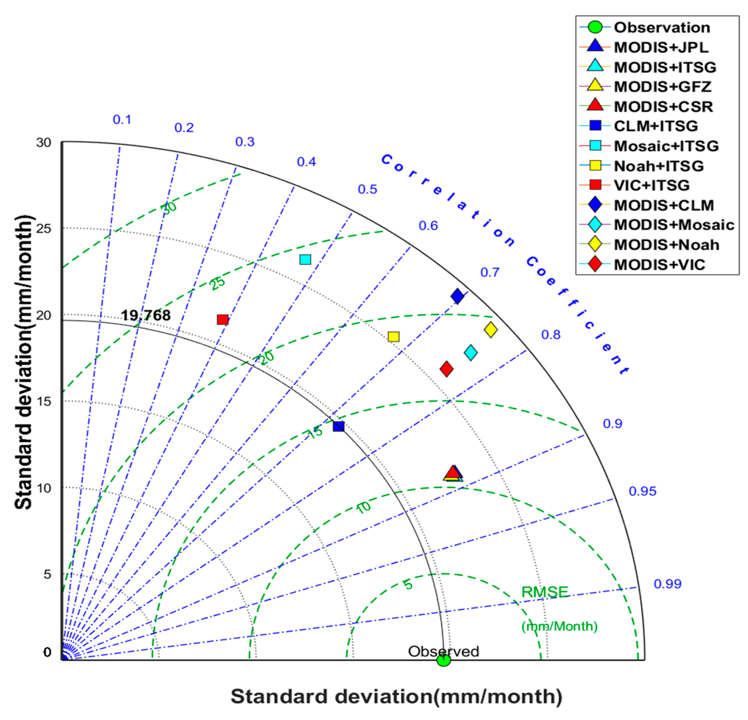
The Taylor’s diagram provides a direct way to determine the degree of correspondence between observed and estimated data [90]: it shows the correlation, the RMSE difference, and the standard deviation between two types of data. Figure 8 displayed that four different remotely sensed R derived through the purely data-driven method (triangles) overlapped each other: this indicates that the choice of different GRACE S in combination with the MODIS ET data has a negligible effect on the estimated R. However, the results derived from the MODIS ET and GLDAS S, and GLDAS ET and GRACE S datasets, showed poor consistency, in particular the latter one. These results highlight that the ET is likely the most significant error source during the estimation of the remotely sensed R. In summary, the remotely sensed R derived from the purely data-driven method is the closest to the observed R.

The discrepancy between the observed and evaluated runoff was examined in detail by computing the mean monthly R derived from the three dataset combinations. The results derived from the purely data-driven method best matched those of the observations: the estimated R values for different seasons match those of the observations with various degrees of accuracies. Our results indicated a maximum and a minimum R in July and January, respectively (Figure 9); however, the estimated minimum R was inconsistent with that observed R, which occurred in February. Apparently, the estimated R was underestimated in winter and overestimated in summer (Figure 9a), likely due to the characteristics of the vegetation cover types, which can influence the calculated MODIS ET in different ways during dry and humid seasons.

In case of the GLDAS ET and ITSG GRACE S combination (Figure 9b), the estimated runoff was underestimated between January and August: the GLDAS ET data were overestimated (Figure 5), likely due to the effect of incoming radiations and temperature, as stated in [51]. The S data derived from the GLDAS land surface model were even less accurate than those described above (Figure 9c): the resulting estimated R displayed its maximum one month earlier than the observed time series, causing an underestimation of the R between July and December.

In general, the correlation coefficients between the estimated and the observed R during spring and autumn were higher than during summer and winter from the three combinations of remotely sensed data (

Table 8. Seasonal statistical assessment of the remotely sensed runoff derived from the comparison between the MODIS evapotranspiration and ITSG GRACE terrestrial water storage (MODIS + ITSG), CLM evapotranspiration and ITSG GRACE terrestrial water storage (CLM + ITSG), and MODIS evapotranspiration and Mosaic terrestrial water storage (MODIS + Mosaic), and the ground-based observed runoff data registered at the Datong station.

	Season	PCC	RMSE	NSE
MODIS + ITSG	Spring	0.76	11.00	0.128
	Summer	0.34	13.21	−0.112
	Autumn	0.76	11.88	0.384
	Winter	0.33	10.50	−6.082
CLM + ITSG	Spring	0.50	19.33	−1.693
	Summer	0.46	19.29	−1.37
	Autumn	0.54	13.13	0.248
	Winter	0.44	8.19	−3.31
MODIS + Mosaic	Spring	0.64	14.61	−0.539
	Summer	0.24	19.77	−1.489
	Autumn	0.29	23.64	−1.441
	Winter	0.06	19.60	−23.654

). These results further confirm our observations based on Figure 9: overall, the rising and falling trends were well captured by our estimated R. The higher correlation coefficients during the spring and autumn months probably derived from an overestimation of the modeled ET and, possibly, by the low temporal resolution of the data at the monthly scale.

5. Conclusions

Previous studies have calculated the time series of monthly TBD (in terms of R) in the YRB by applying the water balance equation to a combination of RS and modeled data products. Here, we applied a data-driven method purely based on RS data. Before the investigation, the remotely sensed data were first validated against the in-situ gauge measurements or the inferred measurements at point locations. This validation process indicated that large uncertainties existed in the modeled data products, as verified when the modeled data products were compared with the observed hydrological data collected from the in situ stations or the inferred data, or when the estimated runoff were compared against the observed runoff.

Our best R (obtained from purely remotely sensed data) and those of Ferreira et al. (2013) [37] against the observed runoff reveal the PCC of 0.89 and 0.74, and the RMSE of 11.69 mm/month and 14.30 mm/month, respectively: our method showed statistically better results. The peak-to-peak correlation values were also calculated: in this sense, our method produced slightly better results than those of Syed et al. (2009) [44] and Ferreira et al. (2013) [37].

Seasonal error characterization was conducted to assess the performance of our method during specific seasons. We found that the remotely sensed TBD did not accurately capture the maximum and minimum runoff values in summer and winter, respectively. This poor performance could be attributed to an overestimation and underestimation of ET, respectively, which depend on the input variables (e.g., vegetation cover types, solar radiation, and temperature) [51]. The ET values tend to be overestimated or underestimated when the input variables are instable, particularly in dry and humid seasons. Notably, the low temporal resolution of the data at a monthly scale could have also contributed to these effects. This finding has not been reported in previous studies.

Satellite data products with higher temporal resolution are gradually becoming available (e.g., daily TRMM precipitation [91], eight-day MODIS evapotranspiration [92], and daily GRACE terrestrial water storage data products [93]). Future research might contemplate the application of our proposed method to these new data, while caution has to be taken with the data validation, data postprocessing steps, and the geographic region.

References

1. Tarpanelli, A.; Barbetta, S.; Brocca, L.; Moramarco, T. River discharge estimation by using altimetry data and simplified flood routing modeling. Remote Sens. 2013, 5, 4145–4162. [Google Scholar] [CrossRef]
2. Oki, T.; Kanae, S. Global hydrological cycles and world water resources. Science 2006, 313, 1068–1072. [Google Scholar] [CrossRef] [PubMed]
3. Hassan, A.A.; Jin, S. Lake level change and total water discharge in east Africa rift valley from satellite-based observations. Glob. Planet. Chang. 2014, 117, 79–90. [Google Scholar] [CrossRef]
4. Huang, S.; Krysanova, V.; Zhai, J.; Su, B. Impact of intensive irrigation activities on river discharge under agricultural scenarios in the semi-arid Aksu river basin, northwest China. Water Resour. Manag. 2015, 29, 945–959. [Google Scholar] [CrossRef]
5. Pauw, K.; Thurlow, J. Economic losses and poverty effects of droughts and floods in Malawi. 2009. Available online: http://ebrary.ifpri.org/utils/getfile/collection/p15738coll2/id/126163/filename/126264.pdf (accessed on 1 August 2019).
6. Zampieri, M.; Carmona Garcia, G.; Dentener, F.; Gumma, M.; Salamon, P.; Seguini, L.; Toreti, A. Surface freshwater limitation explains worst rice production anomaly in India in 2002. Remote Sens. 2018, 10, 244. [Google Scholar] [CrossRef]
7. Sichangi, A.W.; Wang, L.; Yang, K.; Chen, D.; Wang, Z.; Li, X.; Zhou, J.; Liu, W.; Kuria, D. Estimating continental river basin discharges using multiple remote sensing data sets. Remote Sens. Environ. 2016, 179, 36–53. [Google Scholar] [CrossRef] [Green Version]
8. Alsdorf, D.E.; Lettenmaier, D.P. Tracking fresh water from space. Science 2003, 301, 1491–1494. [Google Scholar] [CrossRef] [PubMed]
9. Vörösmarty, C.; Askew, A.; Grabs, W.; Barry, R.; Birkett, C.; Döll, P.; Goodison, B.; Hall, A.; Jenne, R.; Kitaev, L. Global water data: A newly endangered species. Eos Trans. Am. Geophys. Union 2001, 82, 54–58. [Google Scholar] [CrossRef]
10. Sneeuw, N.; Lorenz, C.; Devaraju, B.; Tourian, M.J.; Riegger, J.; Kunstmann, H.; Bardossy, A. Estimating runoff using hydro-geodetic approaches. Surv. Geophys. 2014, 35, 1333–1359. [Google Scholar] [CrossRef]
11. Famiglietti, J.S. Remote sensing of terrestrial water storage, soil moisture and surface waters. In The State of the Planet: Frontiers and Challenges in Geophysics; Geophysical Monograph Series; American Geophysical Union: Washington, DC, USA, 2004; Volume 150, pp. 197–207. [Google Scholar]
12. Smith, L.C. Satellite remote sensing of river inundation area, stage, and discharge: A review. Hydrol. Process. 1997, 11, 1427–1439. [Google Scholar] [CrossRef]
13. Wen, X.; Hu, D.; Cao, B.; Shen, S.; Tang, X. Dynamics change of Honghu lake’s water surface area and its driving force analysis based on remote sensing technique and TOPMODEL model. IOP Conf. Ser. Earth Environ. Sci. 2014, 17, 12130. [Google Scholar] [CrossRef]
14. Townsend, P.A.; Walsh, S.J. Modeling floodplain inundation using an integrated GIS with radar and optical remote sensing. Geomorphology 1998, 21, 295–312. [Google Scholar] [CrossRef]
15. Yue, W.; Xu, J.; Tan, W. The relationship between land surface temperature and NDVI with remote sensing: Application to shanghai Landsat 7 ETM+ data. Int. J. Remote Sens. 2007, 28, 3205–3226. [Google Scholar] [CrossRef]
16. Pan, F.; Nichols, J. Remote sensing of river stage using the cross-sectional inundation area-river stage relationship (IARSR) constructed from digital elevation model data. Hydrol. Process. 2013, 27, 3596–3606. [Google Scholar] [CrossRef]
17. Smith, L.C.; Pavelsky, T.M. Estimation of river discharge, propagation speed, and hydraulic geometry from space: Lena river, Siberia. Water Resour. Res. 2008, 44, 173–175. [Google Scholar] [CrossRef]
18. Tarpanelli, A.; Brocca, L.; Lacava, T.; Faruolo, M.; Melone, F.; Moramarco, T.; Pergola, N.; Tramutoli, V. River discharge estimation through MODIS data. In Remote Sensing for Agriculture Ecosystems Hydrology XIII, International Society for Optics and Photonics; International Society for Optics and Photonics: Washington, DC, USA, 2011; Volume 8174, pp. 283–304. [Google Scholar]
19. Chiara, C.; Marco, M. Calibration and validation of a distributed energy–water balance model using satellite data of land surface temperature and ground discharge measurements. J. Hydrometeorol. 2012, 15, 376–392. [Google Scholar]
20. Lu, X.X.; Wang, J.; Higgitt, D.L. NDVI and its relationships with hydrological regimes in the upper Yangtze. Can. J. Remote Sens. 2000, 26, 418–427. [Google Scholar] [CrossRef]
21. Li, C.H.; Yang, Z.F. Spatio-temporal changes of NDVI and their relations with precipitation and runoff in the Yellow River Basin. Geogr. Res. 2004, 23, 753–759. [Google Scholar]
22. Xu, W.; Yang, D.; Li, Y.; Xiao, R. Correlation analysis of Mackenzie river discharge and NDVI relationship. Can. J. Remote Sens. 2016, 42, 292–306. [Google Scholar] [CrossRef]
23. Leopold, L.B.; Maddock, T. The Hydraulic Geometry of Stream Channels and Some Physiographic Implications; US Government Printing Office: Washington, DC, USA, 1953; Volume 252.
24. Chow, V.T.; Maidment, D.; Mays, L. Applied Hydrology. In Water Resources and Environmental Engineering; McGraw-Hill: Singapore, 1988. [Google Scholar]
25. Bjerklie, D.M.; Moller, D.; Smith, L.C.; Dingman, S.L. Estimating discharge in rivers using remotely sensed hydraulic information. J. Hydrol. 2005, 309, 191–209. [Google Scholar] [CrossRef]
26. LeFavour, G.; Alsdorf, D. Water slope and discharge in the Amazon river estimated using the shuttle radar topography mission digital elevation model. Geophys. Res. Lett. 2005, 32, L17404. [Google Scholar] [CrossRef]
27. Matgen, P.; Schumann, G.; Henry, J.B.; Hoffmann, L.; Pfister, L. Integration of SAR-derived river inundation areas, high-precision topographic data and a river flow model toward near real-time flood management. Int. J. Appl. Earth Obs. 2007, 9, 247–263. [Google Scholar] [CrossRef]
28. Neal, J.; Schumann, G.; Bates, P.; Buytaert, W.; Matgen, P.; Pappenberger, F. A data assimilation approach to discharge estimation from space. Hydrol. Process. 2010, 23, 3641–3649. [Google Scholar] [CrossRef]
29. Pavelsky, T.M.; Durand, M.T.; Andreadis, K.M.; Beighley, R.E.; Paiva, R.C.D.; Allen, G.H.; Miller, Z.F. Assessing the potential global extent of SWOT river discharge observations. J. Hydrol. 2014, 519, 1516–1525. [Google Scholar] [CrossRef]
30. Hirpa, F.A.; Hopson, T.M.; De Groeve, T.; Brakenridge, G.R.; Gebremichael, M.; Restrepo, P.J. Upstream satellite remote sensing for river discharge forecasting: Application to major rivers in South Asia. Remote Sens. Envrion. 2013, 131, 140–151. [Google Scholar] [CrossRef]
31. Shih, S.F.; Rahi, G.S. Seasonal variations of Manning’s roughness coefficient in a subtropical marsh. Trans. ASABE 1982, 25, 116–119. [Google Scholar] [CrossRef]
32. Mailapalli, D.R.; Raghuwanshi, N.S.; Singh, R.; Schmitz, G.H.; Lennartz, F. Spatial and temporal variation of Manning’s roughness coefficient in furrow irrigation. J. Irrig. Drain. Eng. 2008, 134, 185–192. [Google Scholar] [CrossRef]
33. Frappart, F.; Minh, K.D.; L’Hermitte, J.; Cazenave, A.; Ramillien, G.; Le Toan, T.; Mognard-Campbell, N. Water volume change in the lower Mekong from satellite altimetry and imagery data. Geophys. J. Int. 2006, 167, 570–584. [Google Scholar] [CrossRef] [Green Version]
34. Kouraev, A.V.; Zakharova, E.A.; Samain, O.; Mognard, N.M.; Cazenave, A. Ob’river discharge from TOPEX/Poseidon satellite altimetry (1992–2002). Remote Sens. Environ. 2004, 93, 238–245. [Google Scholar] [CrossRef]
35. Birkinshaw, S.J.; O’donnell, G.M.; Moore, P.; Kilsby, C.G.; Fowler, H.J.; Berry, P.A.M. Using satellite altimetry data to augment flow estimation techniques on the Mekong River. Hydrol. Process. 2010, 24, 3811–3825. [Google Scholar] [CrossRef]
36. Sulistioadi, Y.B.; Tseng, K.H.; Shum, C.K.; Hidayat, H.; Sumaryono, M.; Suhardiman, A.; Setiawan, F.; Sunarso, S. Satellite radar altimetry for monitoring small rivers and lakes in Indonesia. Hydrol. Earth Syst. Sci. 2015, 19, 341–359. [Google Scholar] [CrossRef] [Green Version]
37. Ferreira, V.G.; Gong, Z.; He, X.; Zhang, Y.; Andam-Akorful, S.A. Estimating total discharge in the Yangtze River Basin using satellite-based observations. Remote Sens. 2013, 5, 3415–3430. [Google Scholar] [CrossRef]
38. Syed, T.H.; Famiglietti, J.S.; Chen, J.; Rodell, M.; Seneviratne, S.I.; Viterbo, P.; Wilson, C.R. Total basin discharge for the Amazon and Mississippi River basins from GRACE and a land—Atmosphere water balance. Geophys. Res. Lett. 2005, 32. [Google Scholar] [CrossRef]
39. Seneviratne, S.I.; Viterbo, P.; Lüthi, D.; Schär, C. Inferring changes in terrestrial water storage using ERA-40 reanalysis data: The Mississippi River basin. J. Clim. 2004, 17, 2039–2057. [Google Scholar] [CrossRef]
40. Seo, J.; Lee, S.I. Total discharge estimation in the Korean Peninsula using multi-satellite products. Water 2017, 9, 532. [Google Scholar]
41. Oki, T.; Musiake, K.; Matsuyama, H.; Masuda, K. Global atmospheric water balance and runoff from large river basins. Hydrol. Process. 1995, 9, 655–678. [Google Scholar] [CrossRef]
42. Jacob, D. A note to the simulation of the annual and inter-annual variability of the water budget over the Baltic Sea drainage basin. Meteorol. Atmos. Phys. 2001, 77, 61–73. [Google Scholar] [CrossRef]
43. Peixoto, J.P.; Oort, A.H. Physics of climate. N. Y. Am. Inst. Phys. 1992, 173, 415–423. [Google Scholar] [CrossRef]
44. Syed, T.H.; Famiglietti, J.S.; Chambers, D.P. GRACE-based estimates of terrestrial freshwater discharge from basin to continental scales. J. Hydrometeorol. 2009, 10, 22–40. [Google Scholar] [CrossRef]
45. Rodell, M.; Famiglietti, J.S.; Chen, J.; Seneviratne, S.I.; Viterbo, P.; Holl, S.; Wilson, C.R. Basin scale estimates of evapotranspiration using GRACE and other observations. Geophys. Res. Lett. 2004, 31. [Google Scholar] [CrossRef] [Green Version]
46. Roads, J.; Lawford, R.; Bainto, E.; Berbery, E.; Chen, S.; Fekete, B.; Gallo, K.; Grundstein, A.; Higgins, W.; Kanamitsu, M.; et al. GCIP water and energy budget synthesis (WEBS). J. Geophys. Res. Atmos. 2003, 108. [Google Scholar] [CrossRef] [Green Version]
47. Dai, A.; Trenberth, K.E. Estimates of freshwater discharge from continents: Latitudinal and seasonal variations. J. Hydrometeorol. 2002, 3, 660–687. [Google Scholar] [CrossRef]
48. Kalnay, E.; Kanamitsu, M.; Kistler, R.; Collins, W.; Deaven, D.; Gandin, L.; Iredell, M.; Saha, S.; White, G.; Woollen, J.; et al. The NCEP/NCAR 40-year reanalysis project. Bull. Am. Meteorol. Soc. 1996, 77, 437–472. [Google Scholar] [CrossRef]
49. Kummerow, C.; Barnes, W.; Kozu, T.; Shiue, J.; Simpson, J. The tropical rainfall measuring mission (TRMM) sensor package. J. Atmos. Ocean. Technol. 1998, 15, 809–817. [Google Scholar] [CrossRef]
50. Tapley, B.D.; Bettadpur, S.; Ries, J.C.; Thompson, P.F.; Watkins, M.M. GRACE measurements of mass variability in the Earth system. Science 2004, 305, 503–505. [Google Scholar] [CrossRef]
51. Khan, M.S.; Liaqat, U.W.; Baik, J.; Choi, M. Stand-alone uncertainty characterization of GLEAM, GLDAS and MOD16 evapotranspiration products using an extended triple collocation approach. Agric. For. Meteorol. 2018, 252, 256–268. [Google Scholar] [CrossRef]
52. Jiang, T.; Kundzewicz, Z.W.; Su, B. Changes in monthly precipitation and flood hazard in the Yangtze River Basin, China. Int. J. Climatol. A J. R. Meteorol. Soc. 2008, 28, 1471–1481. [Google Scholar] [CrossRef]
53. Zhang, D.; Zhang, Q.; Werner, A.D.; Liu, X. GRACE-based hydrological drought evaluation of the Yangtze River Basin, China. J. Hydrometeorol. 2016, 17, 811–828. [Google Scholar] [CrossRef]
54. Zarfl, C.; Lumsdon, A.E.; Berlekamp, J.; Tydecks, L.; Tockner, K. A global boom in hydropower dam construction. Aquat. Sci. 2015, 77, 161–170. [Google Scholar] [CrossRef]
55. Wang, Y.; Ding, Y.; Ye, B.; Liu, F.; Wang, J. Contributions of climate and human activities to changes in runoff of the Yellow and Yangtze rivers from 1950 to 2008. Sci. China Earth Sci. 2013, 56, 1398–1412. [Google Scholar] [CrossRef]
56. Liu, J.; Zhang, Q.; Singh, V.P.; Shi, P. Contribution of multiple climatic variables and human activities to streamflow changes across China. J. Hydrol. 2017, 545, 145–162. [Google Scholar] [CrossRef] [Green Version]
57. Xi, Y.; Peng, S.; Ciais, P.; Guimberteau, M.; Li, Y.; Piao, S.; Wang, X.; Polcher, J.; Yu, J.; Zhang, X.; et al. Contributions of Climate Change, CO2, Land-Use Change, and Human Activities to Changes in River Flow across 10 Chinese Basins. J. Hydrometeorol. 2018, 19, 1899–1914. [Google Scholar] [CrossRef]
58. Xu, K.; Milliman, J.D.; Xu, H. Temporal trend of precipitation and runoff in major Chinese Rivers since 1951. Glob. Planet. Chang. 2010, 73, 219–232. [Google Scholar] [CrossRef]
59. Zhang, Q.; Chen, G.; Su, B.; Disse, M.; Jiang, T.; Xu, C.Y. Periodicity of sediment load and runoff in the Yangtze River basin and possible impacts of climatic changes and human activities. Hydrol. Sci. J. 2008, 53, 457–465. [Google Scholar] [CrossRef]
60. Zhang, Q.; Xu, C.Y.; Becker, S.; Jiang, T. Sediment and runoff changes in the Yangtze River basin during past 50 years. J. Hydrol. 2006, 331, 511–523. [Google Scholar] [CrossRef]
61. Xu, K.; Milliman, J.D. Seasonal variations of sediment discharge from the Yangtze River before and after impoundment of the Three Gorges Dam. Geomorphology 2009, 104, 276–283. [Google Scholar] [CrossRef]
62. Lyu, Y.; Zheng, S.; Tan, G.; Shu, C. Effects of Three Gorges Dam operation on spatial distribution and evolution of channel thalweg in the Yichang-Chenglingji Reach of the Middle Yangtze River, China. J. Hydrol. 2018, 565, 429–442. [Google Scholar] [CrossRef]
63. Huang, Y.; Salama, M.S.; Krol, M.S.; Van Der, V.; Velde, R.; Hoekstra, A.Y.; Zhou, Y.; Su, Z. Analysis of long-term terrestrial water storage variations in the Yangtze River basin. Hydrol. Earth Syst. Sci. 2013, 17, 1985. [Google Scholar] [CrossRef]
64. Zhang, Q.; Jiang, T.; Gemmer, M.; Becker, S. Precipitation, temperature and runoff analysis from 1950 to 2002 in the Yangtze basin, China. Hydrol. Sci. J. 2005, 50. [Google Scholar] [CrossRef]
65. Zhang, Q.; Xu, C.Y.; Jiang, T.; Wu, Y. Possible influence of ENSO on annual maximum streamflow of the Yangtze River, China. J. Hydrol. 2007, 333, 265–274. [Google Scholar] [CrossRef]
66. Chen, Z.; Li, J.; Shen, H.; Zhanghua, W. Yangtze River of China: Historical analysis of discharge variability and sediment flux. Geomorphology 2001, 41, 77–91. [Google Scholar] [CrossRef]
67. Zhao, G.J.; Hörmann, G.; Fohrer, N.; Gao, J.F.; Zhai, J.Q.; Zhang, Z.X. Spatial and temporal characteristics of wet spells in the Yangtze River Basin from 1961 to 2003. Theor. Appl. Clim. 2009, 98, 107–117. [Google Scholar] [CrossRef]
68. Ding, Y.; Chan, J.C. The East Asian summer monsoon: An overview. Meteorol. Atmos. Phys. 2005, 89, 117–142. [Google Scholar]
69. Su, B.D.; Jiang, T.; Jin, W.B. Recent trends in observed temperature and precipitation extremes in the Yangtze River basin, China. Theor. Appl. Climatol. 2006, 83, 139–151. [Google Scholar] [CrossRef]
70. Yu, F.; Chen, Z.; Ren, X.; Yang, G. Analysis of historical floods on the Yangtze River, China: Characteristics and explanations. Geomorphology 2009, 113, 210–216. [Google Scholar] [CrossRef]
71. Chen, Z.; Zhao, Y. Impact on the Yangtze (Changjiang) estuary from its drainage basin: Sediment load and discharge. Chin. Sci. Bull. 2001, 46, 73–80. [Google Scholar] [CrossRef]
72. Zhang, L.; Dawes, W.R.; Walker, G.R. Response of mean annual evapotranspiration to vegetation changes at catchment scale. Water Resour. Res. 2001, 37, 701–708. [Google Scholar] [CrossRef]
73. Nash, J.E.; Sutcliffe, J.V. River flow forecasting through conceptual models part I—A discussion of principles. J. Hydrol. 1970, 10, 282–290. [Google Scholar] [CrossRef]
74. Liu, Z.; Ostrenga, D.; Teng, W.; Kempler, S. Tropical Rainfall Measuring Mission (TRMM) precipitation data and services for research and applications. Bull. Am. Meteorol. Soc. 2012, 93, 1317–1325. [Google Scholar] [CrossRef]
75. Huffman, G.J. Estimates of root-mean-square random error for finite samples of estimated precipitation. J. Appl. Meteorol. 1997, 36, 1191–1201. [Google Scholar] [CrossRef]
76. Huffman, G.J.; Adler, R.F.; Bolvin, D.T.; Gu, G.; Nelkin, E.J.; Bowman, K.P.; Hong, Y.; Stocker, E.F.; Wolff, D.B. The TRMM Multi-satellite Precipitation Analysis: Quasi-Global, Multi-Year, Combined-Sensor Precipitation Estimates at Fine Scale. J. Hydrometeor. 2007, 8, 38–55. [Google Scholar] [CrossRef]
77. Huffman, G.J.; Adler, R.F.; Bolvin, D.T.; Nelkin, E.J. The TRMM multi-satellite precipitation analysis (TMPA). In Satellite Rainfall Applications for Surface Hydrology; Springer: Dordrecht, The Netherlands, 2010; pp. 3–22. [Google Scholar]
78. Zhang, K.; Kimball, J.S.; Nemani, R.R.; Running, S.W. A continuous satellite-derived global record of land surface evapotranspiration from 1983 to 2006. Water Resour. Res. 2010, 46. [Google Scholar] [CrossRef] [Green Version]
79. Mu, Q.; Zhao, M.; Running, S.W. Improvements to a MODIS global terrestrial evapotranspiration algorithm. Remote Sens. Environ. 2011, 115, 1781–1800. [Google Scholar] [CrossRef]
80. Long, D.; Longuevergne, L.; Scanlon, B.R. Uncertainty in evapotranspiration from land surface modeling, remote sensing, and GRACE satellites. Water Resour. Res. 2014, 50, 1131–1151. [Google Scholar] [CrossRef] [Green Version]
81. Wang, K.; Dickinson, R.E. A review of global terrestrial evapotranspiration: Observation, modeling, climatology, and climatic variability. Rev. Geophys. 2012, 50. [Google Scholar] [CrossRef]
82. GeoForschungsZentrum (GFZ). GRACE Level-2 Release 05 (RL05) Monthly Gravity Field. Available online: http://rz-vm 152.gfz-potsdam.de/grace/ (accessed on 18 May 2018).
83. Swenson, S.; Chambers, D.; Wahr, J. Estimating geocenter variations from a combination of grace and ocean model output. J. Geophys. Res. 2008, 113. [Google Scholar] [CrossRef]
84. Cheng, M.; Tapley, B.D. Variations in the Earth’s oblateness during the past 28 years. J. Geophys Res. 2004, 109. [Google Scholar] [CrossRef]
85. Ramillien, G.; Frappart, F.; Cazenave, A.; Güntner, A. Time variations of land water storage from an inversion of 2 years of GRACE geoids. Earth. Planet. Sci. Lett. 2005, 235, 283–301. [Google Scholar] [CrossRef] [Green Version]
86. Swenson, S.; Wahr, J. Post--processing removal of correlated errors in GRACE data. Geophys. Res. Lett. 2006, 33. [Google Scholar] [CrossRef]
87. Wahr, J.; Molenaar, M.; Bryan, F. Time variability of the Earth’s gravity field: Hydrological and oceanic effects and their possible detection using GRACE. J. Geophys. Res. Solid Earth 1998, 103, 30205–30229. [Google Scholar] [CrossRef]
88. Syed, T.H.; Famiglietti, J.S.; Rodell, M.; Chen, J.; Wilson, C.R. Analysis of terrestrial water storage changes from GRACE and GLDAS. Water Resour. Res. 2008, 44. [Google Scholar] [CrossRef]
89. Yang, T.; Wang, C.; Yu, Z.; Xu, F. Characterization of spatio-temporal patterns for various GRACE-and GLDAS-born estimates for changes of global terrestrial water storage. Glob. Planet. Chang. 2013, 109, 30–37. [Google Scholar] [CrossRef]
90. Taylor, K.E. Summarizing multiple aspects of model performance in a single diagram. J. Geophys. Res. Atmos. 2001, 106, 7183–7192. [Google Scholar] [CrossRef]
91. Huffffman, G.J.; Bolvin, D.T. Real-Time TRMM Multi-Satellite Precipitation Analysis Data Set Documentation; NASA Tech Doc, 2015. Available online: https://docserver.gesdisc.eosdis.nasa.gov/public/project/GPM/3B4XRT_doc_V7.pdf (accessed on 1 August 2019).
92. Running, S.; Mu, Q.; Zhao, M. MYD16A2 MODIS/Aqua Net Evapotranspiration 8-Day L4 Global 500m SIN Grid V006 [Data Set]; NASA EOSDIS Land Processes DAAC. 2017. Available online: https://lpdaac.usgs.gov/documents/378/MOD16_User_Guide_V6.pdf (accessed on 1 August 2019).
93. Gouweleeuw, B.T.; Kvas, A.; Gruber, C.; Gain, A.K.; Mayer-Gürr, T.; Flechtner, F.; Güntner, A. Daily GRACE gravity field solutions track major flood events in the Ganges–Brahmaputra Delta. Hydrol. Earth Syst. Sci. 2018, 22, 2867–2880. [Google Scholar] [CrossRef]
Figure 1. Map of the Yangtze River basin (YRB). Selected hydrological stations (red stars), which collected precipitation, evaporation, and discharge data time series, are situated along the upper, middle, and lower reaches of the Yangtze River. The point locations (black dots) correspond to grid values included in the estimated basin-averaged runoff.
Sensors 19 03386 g001
Figure 2. Monthly runoff time series, averaged from the daily discharge data collected at the Datong station (and divided by the basin area).
Sensors 19 03386 g002
Figure 3. TRMM and observation precipitation time series in correspondence of the (a) Pingshan (upper reaches), (b) Chenglingji (middle reaches), and (c) Datong (lower reaches) stations.
Sensors 19 03386 g003aSensors 19 03386 g003b
Figure 4. MODIS evapotranspiration and inferred evapotranspiration from observed evaporation data time series in correspondence of (a) Pingshan (upper reaches), (b) Chenglingji (middle reaches), and (c) Datong (lower reaches) stations.
Sensors 19 03386 g004aSensors 19 03386 g004b
Figure 5. MODIS and GLDAS modeled evapotranspiration time series in correspondence of (a) Pingshan (upper reaches), (b) Chenglingji (middle reaches), and (c) Datong (lower reaches) stations.
Sensors 19 03386 g005aSensors 19 03386 g005b
Figure 6. GRACE terrestrial water storage and the GLDAS-modeled time series in correspondence of (a) Pingshan (upper reaches), (b) Chenglingji (middle reaches), and (c) Datong (lower reaches) stations.
Sensors 19 03386 g006
Figure 7. Remotely sensed runoff for the Yangtze river basin derived from the MODIS evapotranspiration and ITSG GRACE terrestrial water storage, CLM evapotranspiration and ITSG GRACE terrestrial water storage, and MODIS evapotranspiration and Mosaic terrestrial water storage datasets.
Sensors 19 03386 g007
Figure 8. Taylor’s diagram showing the statistics results obtained from the comparison between the observed (green circle) and remotely sensed runoff in the Yangtze River Basin (derived from the MODIS evapotranspiration and several GRACE terrestrial water storage (triangles), several GLDAS evapotranspiration and ITSG GRACE terrestrial water storage (squares), and the MODIS evapotranspiration and several GLDAS water storage (diamonds) data.
Sensors 19 03386 g008
Figure 9. Mean monthly runoff in the Yangtze river basin derived from (a) MODIS evapotranspiration and several GRACE terrestrial water storage; (b) several GLDAS evapotranspiration and ITSG GRACE terrestrial water storage; and (c) MODIS evapotranspiration and several GLDAS terrestrial water storage data.
Sensors 19 03386 g009