1. Introduction
Millimeter Wave (mmWave) communication systems are envisioned as integral part of the 5th generation (5G) of mobile telephony. The interest in mmWave transmission comes from the high bandwidth available, allowing for high-throughput links [
1,
2]. Due to the higher carrier frequency, mmWave is expected to provide highly directive transmissions, for example, through adaptive antenna arrays. These directive antennas act as spatial filters and allow for techniques such as beam steering [
3] and Orbital Angular Momentum (OAM) multiplexing [
4]. The predicted benefits have prompted interest in using the technology also in vehicular settings, where demands for communications are currently increasing, in both safety as well as infotainment applications [
5,
6,
7]. These vehicular settings are well known for their challenging properties even in the sub-6 GHz band. Among these properties are large delay spreads, high non-stationarity and large Doppler spreads [
8]. The challenge is even more pronounced for very high carrier frequencies [
9], as the Doppler effect scales linearly with the carrier frequency [
10]. This amplifies the influence of Root Mean Squared (RMS) Doppler spreads when omni-directional antennas are used [
11,
12,
13].
For sub-
GHz communications, several benchmarking and evaluation mechanisms for Vehicle-to-Everything (V2X) networks have been established. Most prominently, network simulation tools are used to simulate the performance of the network layer [
14,
15]. These tools mainly analyze the protocol performance, and often assume very simple models of the underlying channel. Furthermore, measurement campaigns are often used to assess the performance [
16]. While they are essential for analysis, these have the problem, especially in vehicular settings, that they lack reproducibility of the exact scenarios due to the highly dynamic nature of the vehicular channel, and the many unknown parameters, such as weather and scatterer position. Finally, as a compromise that allows reproducibility, while still capturing the physical properties and the use of real hardware, channel emulation has been used as tool to assess communication performance [
17,
18]. Channel emulation has proven a valuable tool, but it faces new design challenges for mmWave communications.
At sub-
GHz, ad-hoc nodes are equipped with omnidirectional antennas, at least in the plane of interest, i.e., the horizontal plane in vehicular scenarios. The channel to be modeled and emulated becomes largely independent of the equipped antennas. Conversely, due to the high directivity of mmWave communications, different antenna patterns are to be expected. Hence, the channel characteristics observed by the communicating nodes are strongly dependent on the used antenna configurations. For instance, the RMS Doppler spread depends strongly on whether beamforming is performed [
13]. Thus, incorporating antennas in the emulation approach becomes a necessity at mmWave frequencies. This also means that the observed channel, when including antennas, will exhibit sparse properties. Given suitable antennas, the vehicular mmWave channel will be sparse, or show a sparse amount of clusters. This in turn lends itself very well to emulation. Therefore, analyzing the mmWave vehicular channel based on realistic measurement setups, as well as considerations of what to model are of utmost importance. On the other hand, hardware channel emulation poses a limit on the implementation complexity, hence a compromise between fidelity and complexity is required. In the following section, we give a short introduction on how these properties factor into the emulation.
1.1. Channel Emulation
Channel emulation aims at following the process in
Figure 1 to provide a communication channel representative of a channel vehicles encounter on the road. The propagation conditions are mapped to a signal representation, and this signal is then used in hardware to apply the modeled channel to an incoming transmission signal, and forward the resulting output to the receiver. Vehicular channel emulation can be broadly split into three categories of varying abstraction: measurement playback, geometry-based emulation and model-based emulation.
Measurement playback means that the hardware attempts at replaying previously recorded channel sounder data as faithfully as possible [
17]. The advantage of this approach is that no statistical model assumptions have to be introduced, and uncertainty only stems from the measurements themselves, and approximations that might be necessary. The downside of the approach on the other hand is that the measured channel is not inherently representative of a larger scenario. In this case, the importance of Stage (
b) is reduced as much as possible, ideally making it a completely transparent adaption from (
a) to (
c). In the case of mmWave, this is only representative for the chosen antenna setup.
Geometry-based channel emulation generates a vehicular channel from geometric data, employing tools such as Geometry-based Stochastic Channel Model (GSCMs) [
18,
19]. Alternatively, raytracing could be applied [
20,
21]. While these types have to make model assumptions to arrive at emulation, the benefit of this approach is that it can be executed online. As the geometry can be simulated live, an implementation that is sufficiently fast can translate the geometry to emulation at runtime, and thus provide reactive channel emulations that allow virtual drive tests. Here, Stages (
a) and (
b) are equally important and have to be modeled in conjunction. For mmWave, it is crucial to model the antenna position and orientation as part of Stage (
a).
Model based channel emulation is based on stochastic channel models (e.g., [
22]). If done correctly, such models may be representative for a whole class of scenarios, making the emulation results very interesting. Furthermore, due to the stochastic simplifications, these models tend to be of low complexity to implement in hardware. The downside of such model-based emulation is that the emulation quality is completely dependent on the model quality, and is highly challenging to adapt to more specific scenarios. For example, a typical urban channel model is usually not representative of turning a corner. Here, the emulator is completely defined at Stage (
b), and Stage (
a) channel measurements are only taken into account as validation and for tuning purposes, not as a model driving influence. This approach is not as strongly tied to the antenna positions as the other approaches, however very good models are needed to accurately capture the antenna effects.
In all cases, the channel modeling step differs from the an approach that is targeted towards analytical or simulation applications. Due to the necessity of hardware implementation, the model complexity, or model order, directly factors into the emulation step much more stringently than otherwise. Hardware channel emulators, by design, can support limited complexity, and thus every model has to be evaluated not only with respect to accuracy, but also to complexity.
1.2. Literature Review
Numerous measurement campaigns have studied the mmWave channel both indoors [
23,
24,
25] and for outdoor vehicular channels [
26,
27,
28]. These measurements frequently demonstrate a cluster structure in the impulse response. This cluster-shape was modeled by Saleh and Valenzuela [
29] for wideband channels, and is frequently observed in wireless channels. Similar results are demonstrated in [
30]. These results show that, while many multipaths are seen in mmWave channels, they can be clustered in a small number of scattering clusters, resulting in a cluster-sparse structure. This has been used by the authors of [
31] through applying sparse methods to identify cluster positions for indoor measurements in the frequency range of 2–8 GHz. However, none of those descriptions focused on low complexity modeling aspects, or had the goal of finding representations suitable for emulation.
Channel emulation on the other hand has only been conducted on sub-
GHz channels. Results have been shown for measurement playback [
17], geometric emulation [
18,
19], as well as model based emulation [
32]. Furthermore, Field-Programmable Gate Array (FPGA) implementations are presented in [
33].
Finally, very little analysis on the required model order of the mmWave channel has been conducted. The authors of [
31] used sparse techniques to estimate a mmWave indoor channel, suggesting that a similar approach can work on outdoor channels. At this point, neither mmWave hardware channel emulation nor a theoretical description of the process has been published.
1.3. Our Contribution
In this paper, we present a framework to find a signal representation of channel sounding data that is applicable in hardware emulation setups for mmWave channels. We present a formulation based on the Complex Least Absolute Shrinkage and Selection Operator (LASSO) (c-LASSO) [
34] that finds the best signal representation in the Mean Squared Error (MSE) sense under the side constraint that only
M degrees of freedom are to be used. We present the algorithm using two basis expansions, the Fourier basis, as well as a subband-projected version of the Fourier basis. We demonstrate that the subband-projected Fourier basis is a simple, yet accurate basis to represent clustered channel impulse responses. We furthermore introduce general mechanics to implement sequential estimation which enforces geometric consistency of scattering objects [
34,
35]. We apply these algorithms to two sets of data. On the one hand, we use the Saleh–Valenzuela channel model [
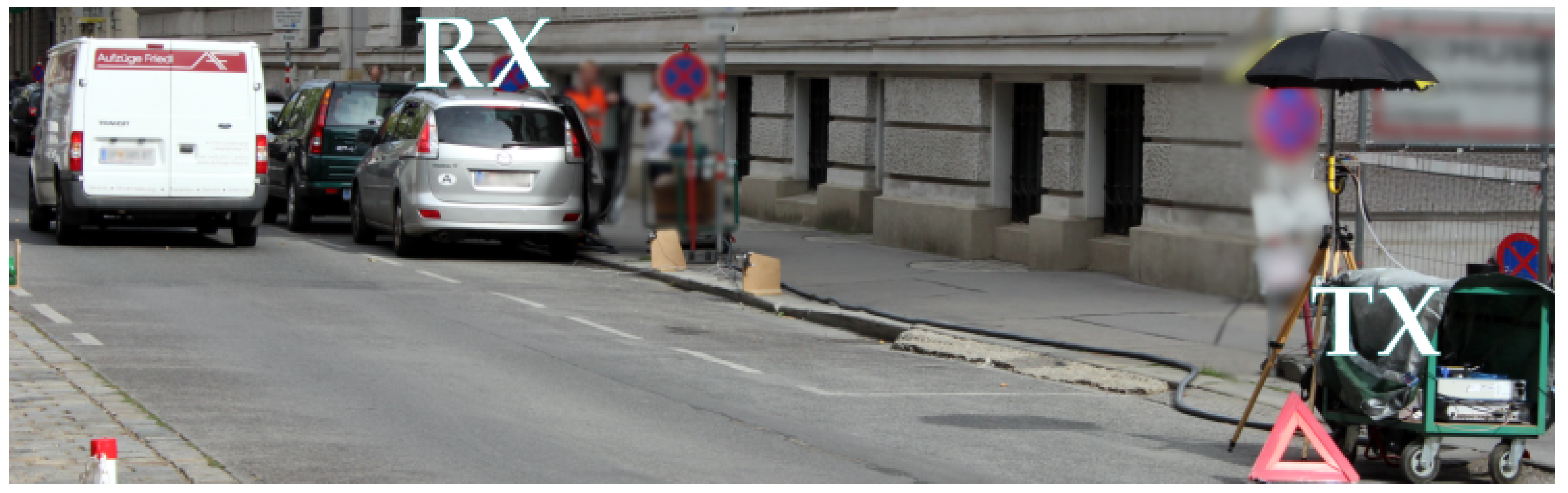
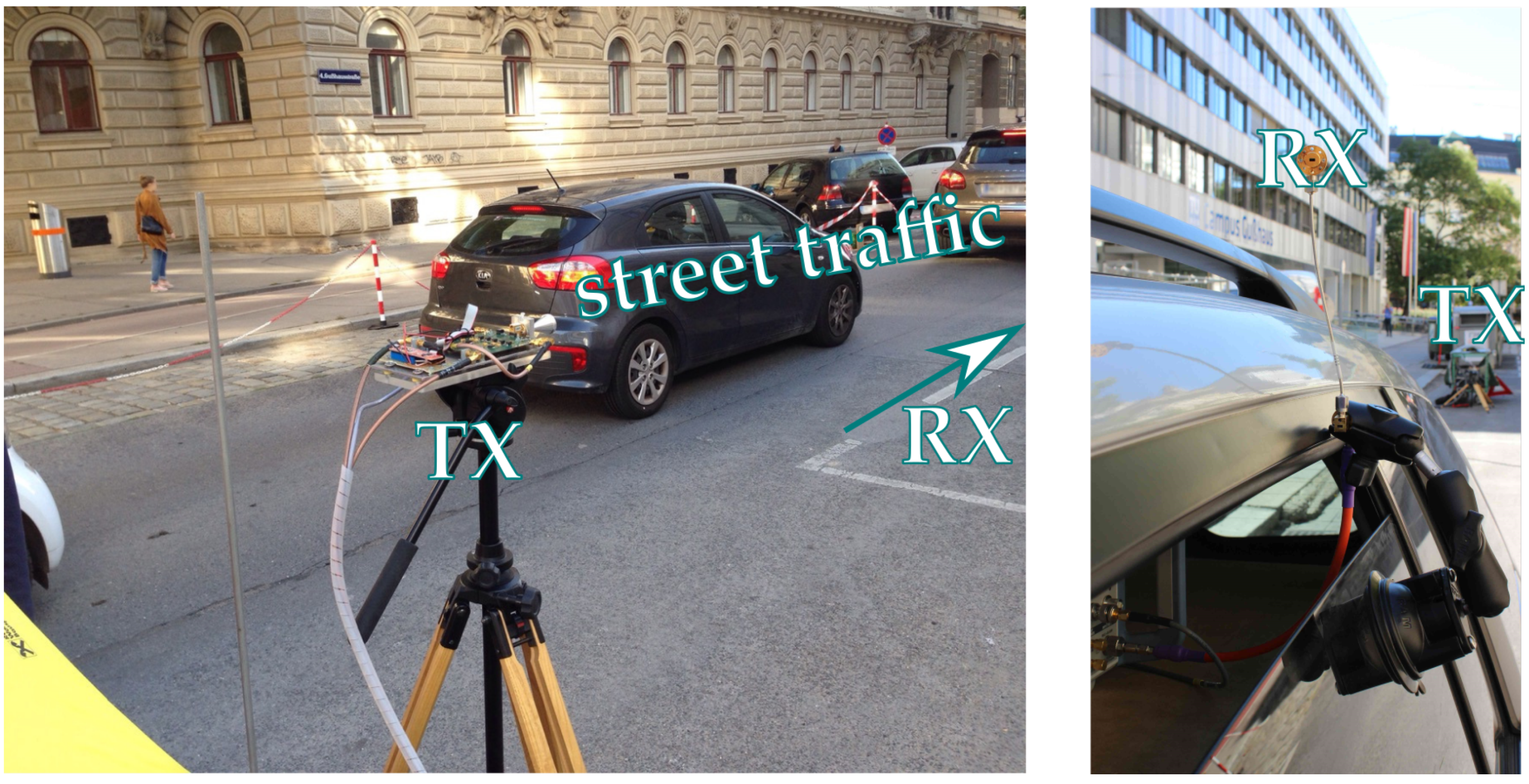
29] to demonstrate the performance of our algorithms on synthetic cluster-channel data. This analysis demonstrates that the subband-filtered Fourier basis is indeed well equipped to represent clustered channel data, especially if the multipaths are densely packed within the clusters. On the other hand, we apply the algorithms to vehicle-to-vehicle (V2V) mmWave measurements conducted in Vienna [
28]. To evaluate not only the fitting performance, but also the fitting-model order trade-off, we propose to use the MSE, as well as the Akaike Information Criterion (AIC) to assess performance [
36]. The AIC is an information theoretic measure that penalizes increase of the model order, to find the optimal trade-off between model order and fitting quality. Here, our results show that the clustering approach works as well as on the synthetic data, suggesting that the channel is indeed clustered. Furthermore, the AIC indicates optimal fitting trade-off at 4–6 clusters, which agrees very well with the physical interpretation of the measurement setup.
The presented framework is formulated as general as possible, and not tied to the vehicular scenario. However, our considerations and optimizations with respect to channel sparsity, clustering and scatterer mobility are targeted at the characteristics of a vehicular scenario. While this work only presents a direct approach to measurement playback, the AIC based model order evaluation provides important insights on the required complexity of stochastic models.
1.4. Notation
Matrices and vectors are denoted by bold letters. Entries of matrices or vectors are indexed via square brackets, such as . Matrix or vector size is indicated via superscripts, for example, , whenever necessary. The all zeros vector (matrix) is expressed by , the all ones vector (matrix) is expressed by and the identity matrix is expressed by . The Euclidean norm is symbolized by , the Manhattan norm by , accordingly. The dagger is used for pseudo inverses, is used for matrix inverses, is used for transposition and is used for conjugate transposition. Kronecker and Hadamard (element-wise) matrix products are denoted by ⊗ and ⊙, respectively. Diag is a function that takes a vector and creates a diagonal matrix with the vector as main diagonal. Finally, peak is a function that returns the magnitude of the kth largest local maximum of the first argument.
2. Reduced Complexity Channel Models and Their Estimation
In general, we describe a communication channel, among other descriptions, as a time-variant frequency selective transfer function
. This description is often used, since it has an immediate interpretation on how frequencies will be attenuated, and how this varies with time. In the case we consider a discrete-time system, we replace the braces by square brackets, resulting in
. Note that, in this case,
t and
f are indices instead of physical quantities. They relate to the physical quantities via the sampling frequency
and arbitrary offsets
and
as
In the remainder of the paper, we only consider discrete-time representations. In this discrete-time domain, we can describe the transfer function which considers N frequency slots at time t by the vector-notation , with .
The major drawback of the transfer-function description is that
is usually not sparse, i.e., there are almost never any zero entries in the vector. This masks the actual required number of model parameters. For example, the studies in [
37,
38] demonstrate a significant improvement in channel estimation quality when using a basis that exhibits sparse properties. Hence, alternative descriptions are of interest. We introduce a general set of
N basis vectors
that we stack into a basis matrix
. Within this basis,
is represented by the basis expansion
Our goal is now to find a basis expansion that results in a sparse structure for , meaning that at most M entries of the vector are not equal to zero. Since this is usually not possible to find exactly, we require to find a basis that minimizes a cost function given a certain sparsity order M. In the following two sections, we present two possible choices for such a basis.
2.1. Tapped Delay Line
The most standard representation besides the time-variant transfer function is the time-variant impulse response , which depends on the time and the delays. The impulse response is sparse exactly if
Only a small number of distinctive MPCs exist.
If many MPCs exist, they are grouped in a small number of clusters. Within these clusters, all MPCs arrive within the same sampling period, resulting in only one resolvable tap.
Then, we can describe the channel impulse response as
Here,
is the time-discrete Dirac function, and
and
are complex amplitude and delay of the
mth tap, respectively. Hence, this model is called the tapped delay line model [
32]. This delay line can again be written in vector notation as function of time
, and is related to
via the Discrete Fourier Transform (DFT) matrix
In our case, we use the unitary, centered definition of the DFT matrix with elements defined as
2.2. Clustered Delay Line
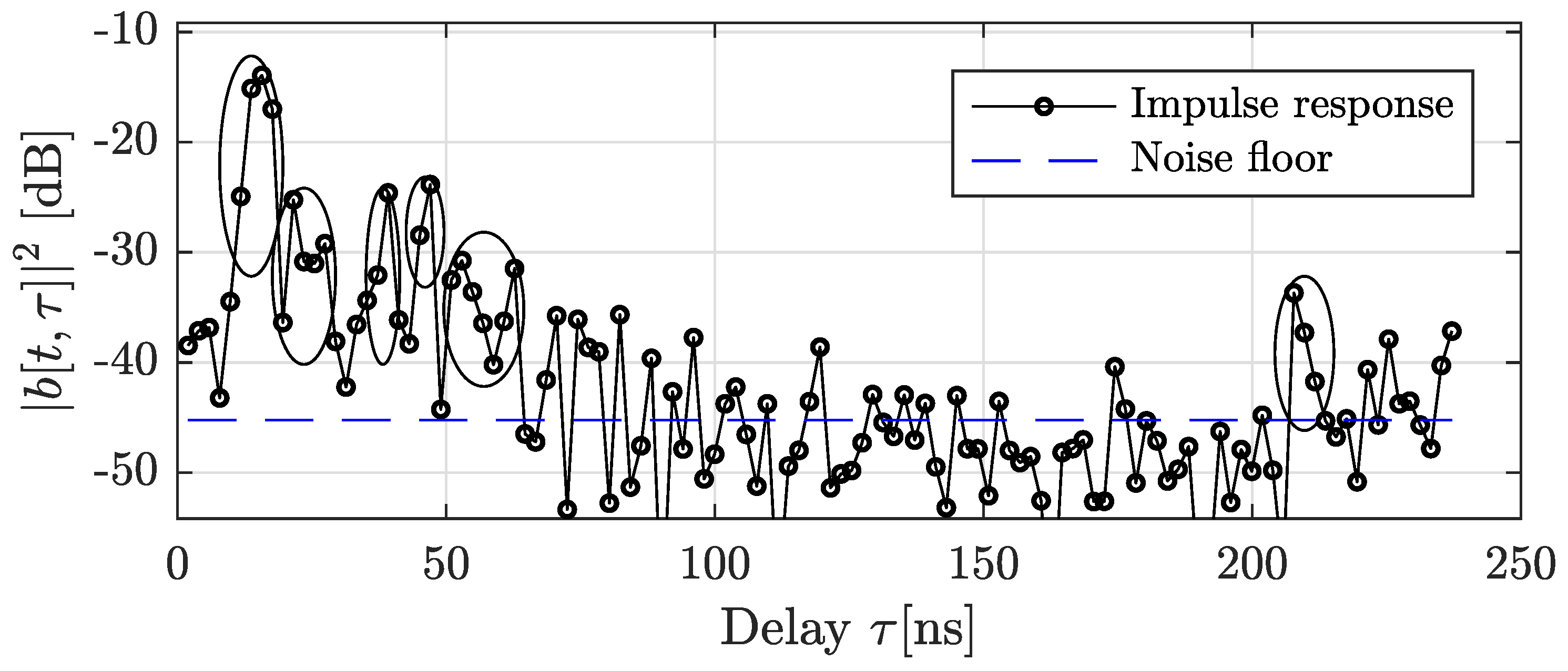
If the MPCs arrive clustered, but the sampling period is too small, the conditions in the previous sections are violated. This happens in wide-band systems, such as typical mmWave systems. Then, we see an impulse response structure such as this
Here,
is the number of clusters,
is the delay of the
kth cluster, and
is the excess delay of the
lth tap within the
kth cluster. The overall sparsity in this case equals
. Of course, we can use the same basis expansion as in
Section 2.1. However, we want to better exploit the cluster structure. A realization of such a cluster response seen in measurements is shown in
Figure 2.
If we project the transfer function on a smaller frequency subband, we reduce the spatial resolution of our system. Thus, more MPCs will coincide on one tap, and the overall structure will be more sparse. We introduce the projection matrix
, which is a diagonal matrix of the structure
with
being the block of considered subcarriers. Here, we impose the considered subcarriers to be adjacent, to achieve bandpass structure. Then, the delay line
which fulfills
will be more sparse for smaller sets of
. We now split the full bandwidth
B into
P orthogonal subbands of equal size
and introduce a separate basis expansion
for each subband
. Now, we introduce the concatenated vector
, as well as the concatenated projected DFT matrix
and present a new basis expansion
For clusters, this has a total sparseness of , however, as be shown below, this basis exploits the cluster structure well, and requires a smaller total model order M than a straightforward tapped-delay line expansion. While remains the same, we demonstrate that P can be chosen significantly smaller than for the same estimation quality.
The resulting estimate can be collapsed into a tapped delay line
via the Inverse DFT (IDFT)
2.3. Sparse Channel Estimation through c-LASSO
Given a channel realization of a transfer function, caused by a sparse basis, which is corrupted by measurement noise
, we estimate the sparse basis expansion
using the c-LASSO [
34,
39], which is defined as
Here,
is a Lagrangian multiplier. The LASSO aims to minimize the MSE (via the squared 2-norm), and enforces sparse solutions through a 1-norm side-constraint.The formulation as given is a convex problem, and is thus solvable by toolboxes such as the cvx toolbox [
40]. Depending on the basis
, and the magnitude of
, a different number of nonzero parameters in different positions will be chosen for
. In [
34], Algorithm 1 was demonstrated which finds a
M-sparse solution given a target
, a basis
by iterating over
until the correct sparsity order is found.
| Algorithm 1 c-LASSO algorithm. |
| 1: | procedurec-LASSO() |
| 2: | | ▹ Tradeoff between speed and convergence |
| 3: | | ▹ Threshold for detecting nonzero magnitudes. |
| 4: | |
| 5: | |
| 6: | while do |
| 7: | |
| 8: | |
| 9: | if then | ▹ Activate additional taps |
| 10: | |
| 11: | | ▹ Set of local maxima above threshold. |
| 12: | + 1 |
| 13: | |
| 14: | else if then | ▹ Deactivate unnecessary taps |
| 15: | bisecting between and . | ▹ For details see [34] |
| 16: | end if |
| 17: | end while |
| 18: | Refine estimate using Equation (16) |
| 19: | return |
| 20: | end procedure |
When the algorithm has found a solution with the correct sparsity, the choice of
may not be optimal in the MSE sense, as the algorithm is biased by the 1-norm. To ensure that, for the resulting active set, the least-squares solution is found, the following refinement step is executed in Line 18
where
is the indicator function that maps a
vector to an
vector with
if
, and
otherwise. This computes a least squares estimate for
that only uses the
M active taps found by the algorithm, and leaves the rest 0.
For the bisection on Line 15, Mecklenbräuker et al. [
34] gave progressive approximations for efficient implementations in Equations (36)–(38). When iterating over a sequence of correlated vectors, such as time snapshots of frequency responses, the output
should be used as initial value
in the subsequent estimation process. In the subsequent sections, we detail several approaches at configuring the algorithm depending on the design goal.
2.3.1. Configuration for Delay Line Estimation
After observing the channel response , we now search for a M-sparse delay line estimate . This is obtained directly by using as basis .
2.3.2. Configuration for Subband Cluster Estimation
We now extend the LASSO to the subband cluster structure from Equation (13). Due to the concatenation of the
P subband impulse responses, we now have to define in what sense we want to ensure sparseness. For this paper, we want to estimate the same level of sparseness
across all subband impulse responses, resulting in a overall sparseness of
. We achieve this by extending the Lagrangian multiplier
to a vector
of size
, and extending the LASSO as follows
Due to the orthogonality of the projections, this formulation can be rewritten as a joint optimization of the subband impulse responses
In this formulation, the sum terms do not depend on each other, hence the optimization can be computed by optimizing every sum term individually. These, however, have the same structure as the c-LASSO and thus be optimized according to Algorithm 1.
2.3.3. Configuration for Sequential Estimation
In the previous sections, we treat the estimation of as an optimization problem completely independent of all other times . We refer to this as memoryless estimation. Now, we want to account for the fact that the delays in the delay lines relate to geometrical positions of scatterers. These are limited in their ability to move between two snapshots, hence the tap positions of adjacent snapshots should reflect this. However, due to noisy observations, the tap positions end up fluctuating strongly in a memoryless estimation.
Therefore, we introduce a sequential approach that tracks prior tap positions and encourages tap consistency in the estimation of the next snapshot. This is done by substituting
, and optimizing for
. As long as
is invertible, it acts as weighting matrix for the nonzero entries in
, encouraging certain taps and discouraging other [
35]. This can be used to encourage consistency of tap positions, similar to [
41]. The weight matrix
is initialized as identity matrix as in the memoryless case. Then, iteratively, the weights are updated for new snapshots according to the following rules.
Propagation of Active Taps
A scatterer can physically move at most
d delay samples between two snapshots. Thus, after calculating an estimate
, we adapt
for all
j that are within
d tap of at least one nonzero entry of
. This will always lower the entry in the diagonal, making it less penalized in the optimization, and thus more likely to be picked again. Here, we ensure that we do not calculate the sum across different partial impulse responses.
Discouraging Spawning New Taps
For all entries that were not modified in the previous step, we apply
This ensures that scarcely activated taps get progressively penalized, ensuring that random noise is less likely to activate such a tap. For the remainder of this paper, we use
, since we work with 2 ns delay resolution and
s snapshot resolution (see
Section 3.2). Due to these numbers, a scatterer can physically only move one tap between snapshots.
Regularization
Finally, on the one hand, we want to ensure stability of the algorithm. We do this by setting the minimum value a diagonal element can take to . Furthermore, we set , as new taps may actually spawn. The values of these parameters can be manipulated to achieve a trade-off between algorithm convergence and geometric consistency.
4. Results
As mentioned above, in our measurements, out of
total subcarriers, only the
center subcarriers carry meaningful data. Hence, we set
, with
This ensures that the unused subcarriers do not factor into the estimation.
4.1. Comparison: Peak Search
To assess our algorithm, we compare it to the performance of
peak search. The estimate is done by calculating the dense impulse response
. Then, all entries except the ones with the largest
M magnitudes are set to 0, resulting in
. Afterwards, we refine the estimate again according to Equation (16), resulting in the
M sparse estimate
If and , the matrix becomes a square orthonormal basis matrix. Under this assumption, the LASSO optimization simplifies to peak search.
4.2. Performance Metrics
4.2.1. Absolute Estimation Quality: Mean Squared Error
We define the MSE as dependent on the bandwidth of interest, defined through
Including the matrix in the MSE is essential to fairly assess fits that are only fit to the targeted subcarriers in .
4.2.2. Balancing Model Order: Akaike Information Criterion
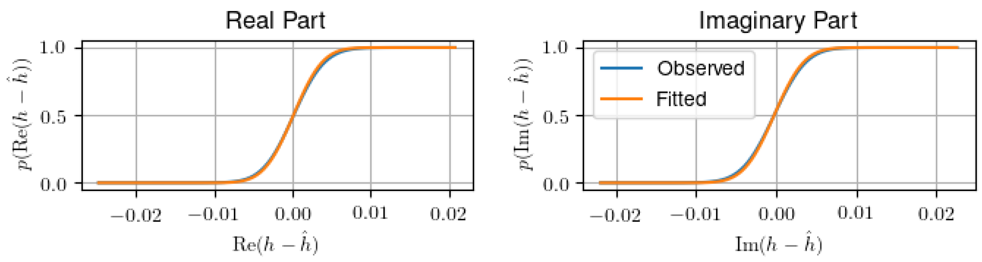
While the MSE is a very commonly used measure, the MSE is ill-equipped to tackle the question of over-fitting, as it does not penalize increasing the model order, and thus always favors higher model order over lower. An important measure that is able to capture the effect of over-fitting is the AIC, which is, for linear regression of Gaussian data, defined as [
36]
RSS denotes the residual sum of squares
, and
denotes the number of estimated frequency samples.
Figure 6 shows that the assumption of Gaussian data is founded, as real and imaginary part of the channel parameters are well fitted by a Gaussian distribution.
For the case where only a small number of parameters is estimated, which is usually given as
[
45], the sample-size corrected AIC is recommended
In our case, every tap has two degrees of freedom (delay and complex value), hence . Thus, we use this corrected criterion as most of our analyzed configurations violate the large parameter number criterion.
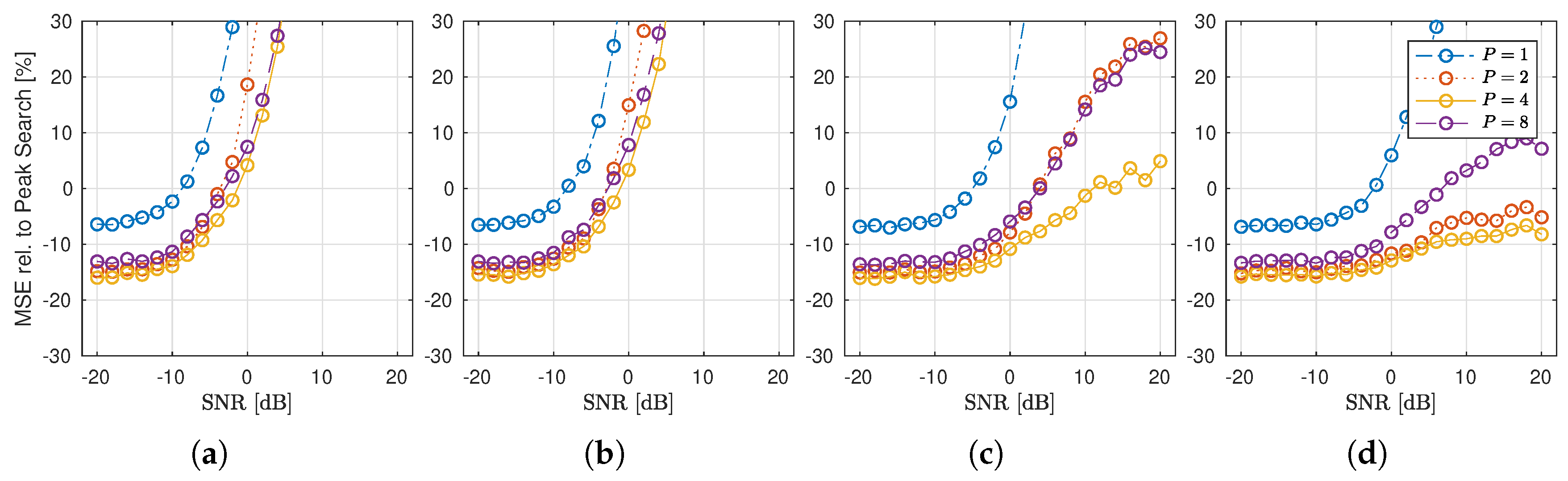
4.3. Performance Analysis for Synthetic Data
Here, we analyze the performance of the c-LASSO algorithm on synthetic data given by the four configurations of the Saleh–Valenzuela model in
Section 3.1. Our main focus here is how well the c-LASSO performs, depending on the
MPC density of the clusters. Since the density of the channel is a design parameter here, the AICs optimum will be itself a function of our model parameter choices, and is of little interest. Instead, we analyze how much improvement over peak search can be achieved, depending on the chosen basis, as well as the channel model configuration. Hence, we analyze the relative change of MSE from
to
In
Figure 7, this relative MSE is plotted in percent (%) from peak search to c-LASSO with
for all four parameter sets over per-subcarrier SNR. All fits, both peak and c-LASSO, have been done with a total of
degrees of freedom. The results show that the LASSO always outperforms peak search in the low SNR-regime, indicating that the c-LASSO works as a more robust estimator than peak search. However, of even more interest to us is, that if the channel model shows
dense MPC clusters (Scenarios (c) and (d)), then, the performance of the c-LASSO improves in the high-SNR regime. For the subband cases of
, the algorithm uniformly outperforms the peak search by at least 10 to 15 throughout the full span. This tells us that our assumption holds, that subband-fitting is able to exploit the signal structure resulting from few MPC clusters that are densely populated to achieve better performance with equal number of degrees of freedom. Finally, the best performance is achieved at
, for
, the performance decreases again.
4.4. Performance Analysis for Channel Sounding Data
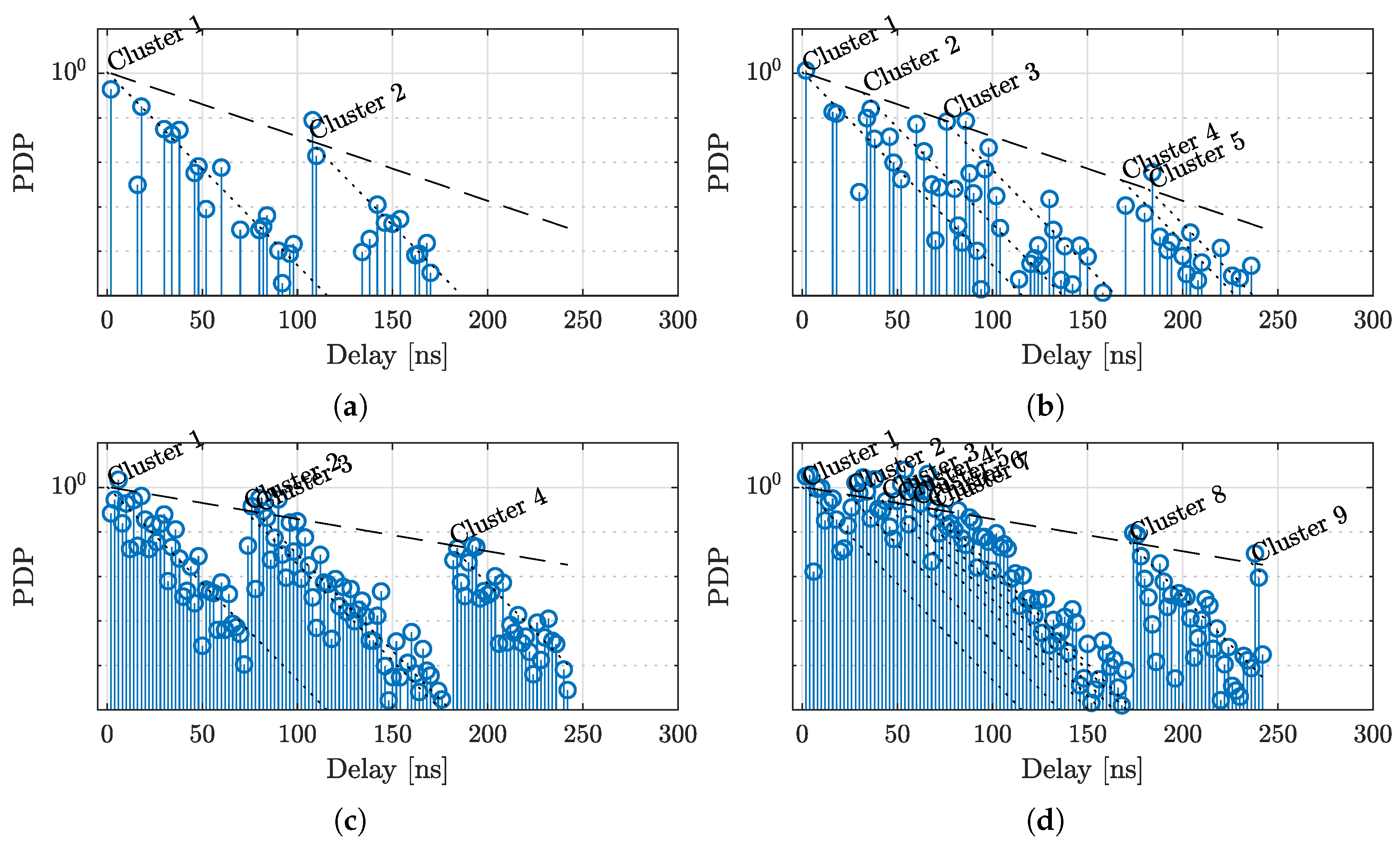
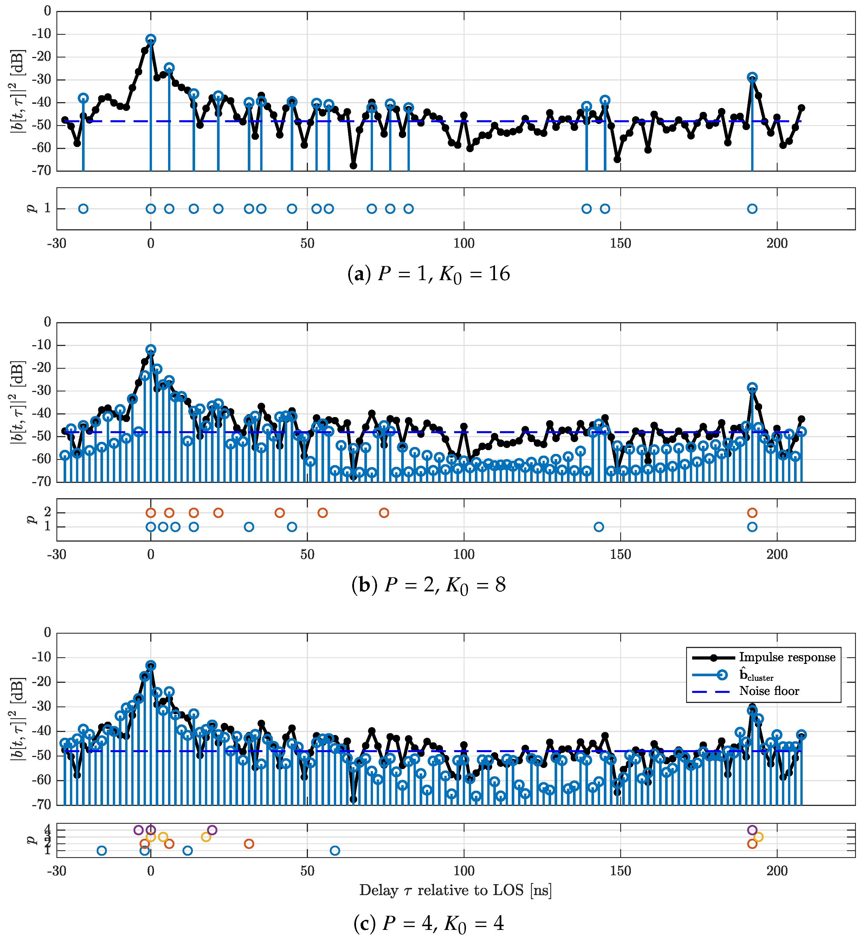
Figure 8 shows an example result for the c-LASSO output. In black, the impulse response calculated from the original channel sounder data is shown. Furthermore, three different configurations for estimations with
are displayed. For each plot, the positions of the
P partial impulse responses are shown below the main plot. Additionally, the cluster impulse response (Equation (
7)) is overlaid, as well as an estimate for the noise floor. We use the median to estimate this noise floor [
46]. The plot illustrates that the impulse response shows clustered shapes, and the subband cluster approach is able to better estimate this cluster structure without expending additional degrees of freedom. The tap positions within the subband responses are highly correlated, relating to the positions of the overall clusters.
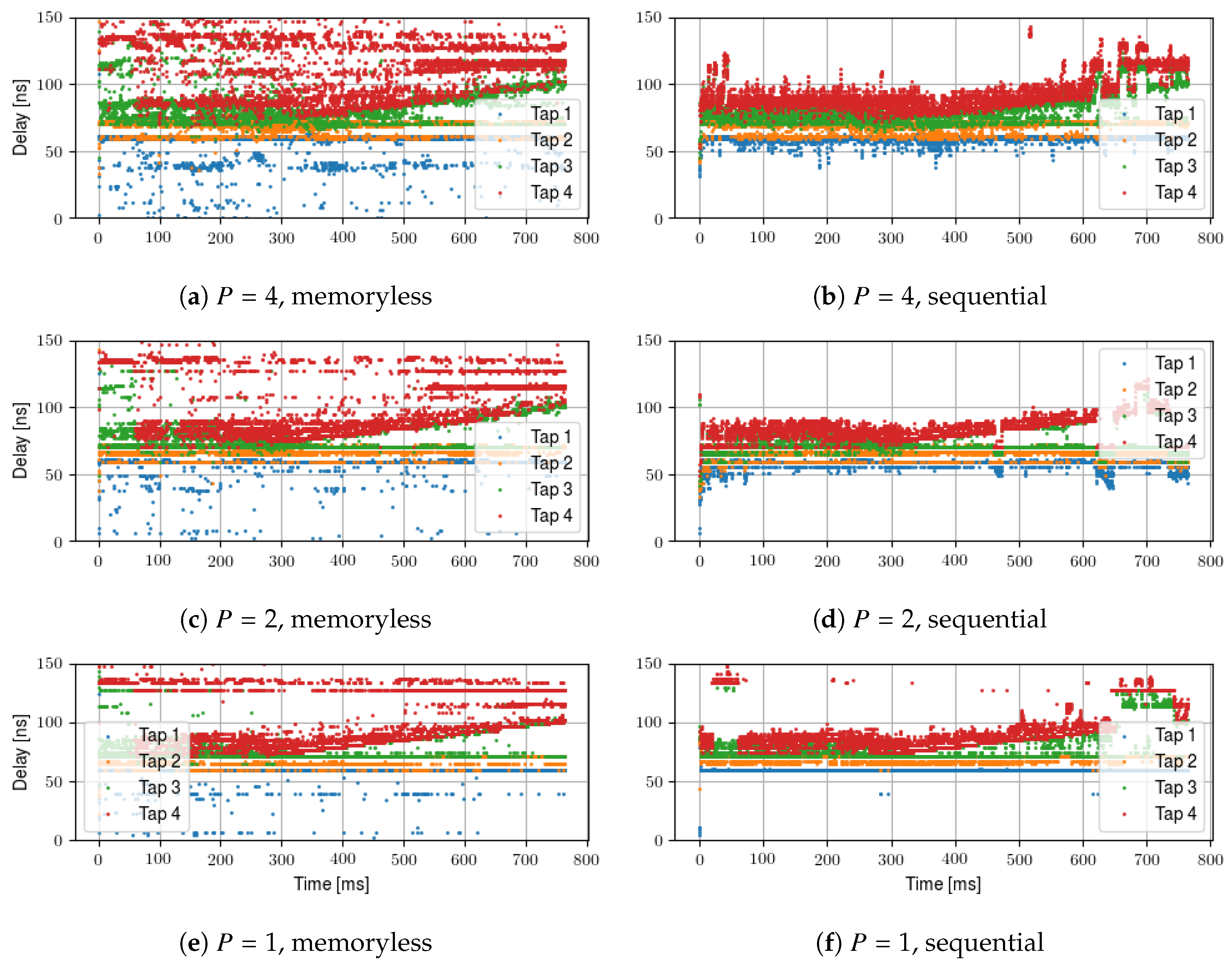
A time evolution of the tap positions of one measurement is shown in
Figure 9. Here, the delays are color coded by arrival time, e.g., the latest estimated tap is always red. To facilitate comparison, we show one partial subband impulse response for every configuration, always with
. The results are shown both for memoryless estimation as well as sequential estimation. The results show that the memoryless estimation shows strong fluctuations of the tap positions within small time spans. Furthermore, for larger
P, the taps tend to be spread out more. This is because of the reduced spatial resolution, which means that close taps are not distinguishable and can be represented by one tap. This allows later tap to be active more likely, as the cluster close to the LOS path collapses and does not use additional taps. In comparison, the sequential estimation effectively reduces the position fluctuations. The taps can still fluctuate in short time spans. For example, a new MPC cluster appears in
Figure 9 at
ms,
ns. At that moment, the fixed amount of taps will be redistributed, and hence the positioning appears to “jump”. However, the overall spatial consistency is drastically improved.
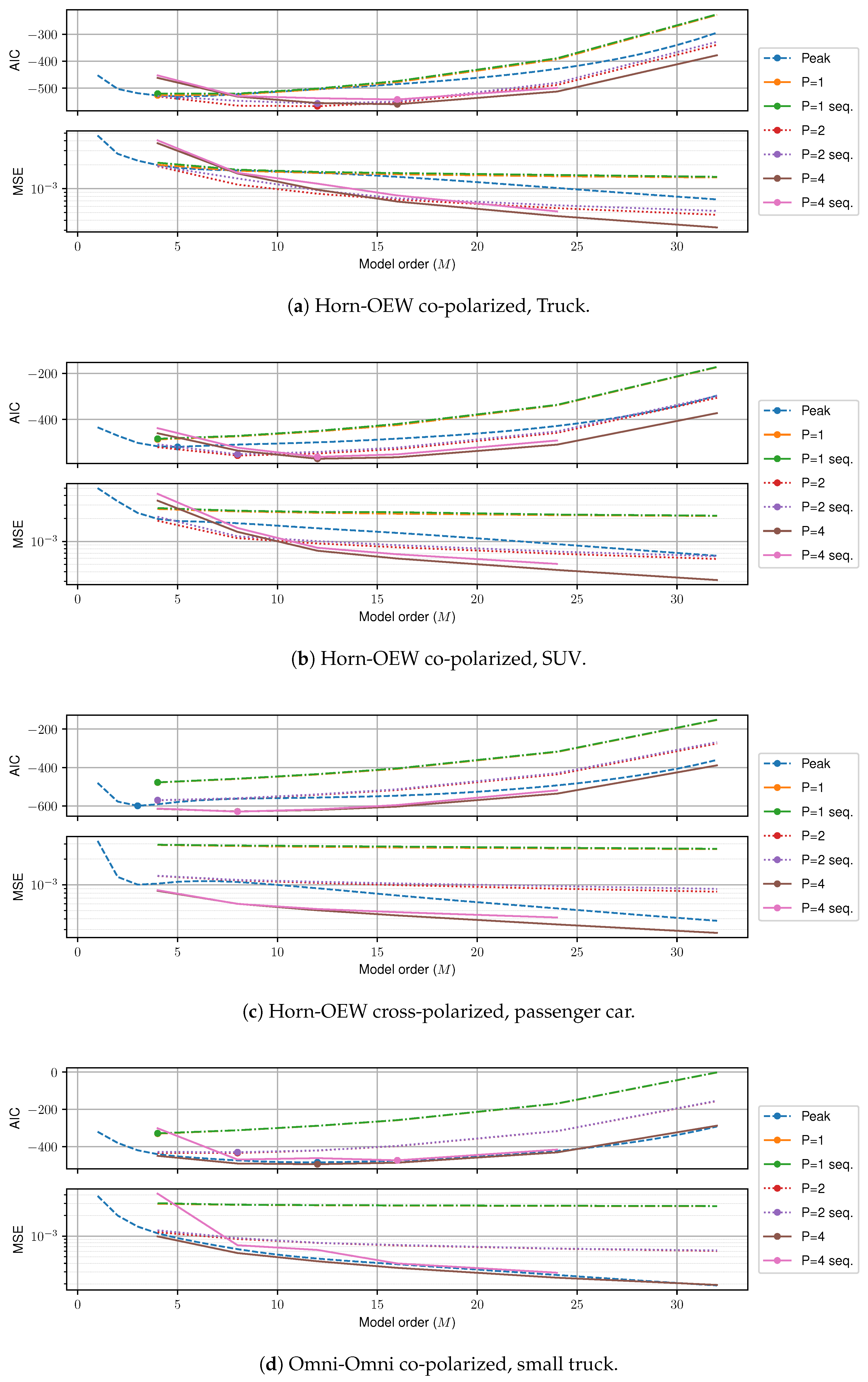
Finally,
Figure 10 shows the MSE and AIC for four different measurement runs. We first consider the fair comparison of the memoryless case with respect to
M. As shown in
Figure 10,
memoryless is uniformly the best estimator for all
M and all measurements. In the case of the Horn-to-Open-Ended Waveguide (OEW) measurements, the gain over peak search is sizeable. Here, the spatial filtering leads to a low number of total clusters, meaning that large gains can be achieved by applying the c-LASSO. On the other hand, for the Omni-to-Omni measurements, the least amount of spatial filtering is applied, and conversely the c-LASSO estimation suffers. However, even for this worst case, the c-LASSO performs at least as well as peak search. In terms of modeling trade-off, the AIC shows a clear minimum (depicted by dots) for all models. The optimal trade-off in terms of AIC is always achieved by the
memoryless c-LASSO at
M between 8 and 16.
Sequential estimation introduces a small MSE-penalty, which is due to the additional side-constraint that we introduced. This penalty is generally very small, and the sequential c-LASSO is the second best LASSO estimator by a large margin, and only for the Omni-to-Omni setup, peak search slightly outperforms the LASSO estimator. However, this comparison is not entirely fair, as peak search never considers spatial consistency.
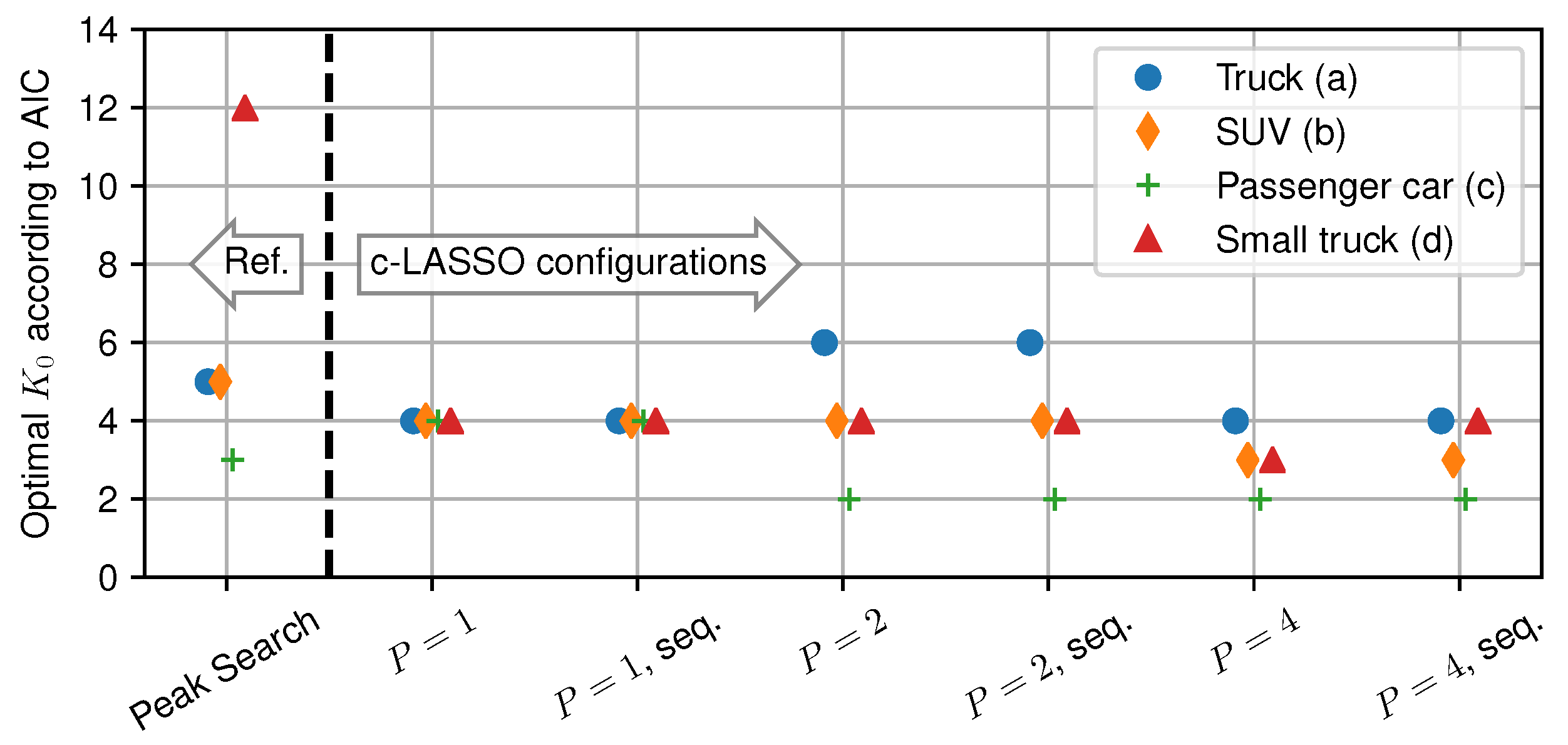
4.5. Discussion: Number of Observed Clusters during the Measurements
Now, we use the AIC to estimate the number of relevant scattering clusters. To analyze this, we take the optimal
M from
Figure 10, and calculate the number of clusters
from it. The results of this for all measurements and estimation configurations are shown in
Figure 11. On the left, the results for peak search are shown, while, on the right, optimal parameters for different c-LASSO settings are demonstrated. Using the normalization with respect to
, we clearly see that all estimation configurations have a consistently small number of relevant multipath clusters. All c-LASSO configurations have the optimal trade-off for
–6 clusters, with the large truck contributing the most clusters. Using the normalization with respect to
, our results show that for the given measurement setup, we never require more than at most six multipath clusters
.
5. Conclusions
When considering emulation of vehicular channels, implementation complexity is always a necessary consideration. Hence, finding a suitably sparse representation of the communication channel is mandatory for high fidelity channel emulation. Due to the large bandwidth in mmWave communications, and the size of vehicles on the road, clustered channel impulse responses are to be expected. If this cluster structure is exploited in the channel modeling approach, the resulting model is shown in this paper to exhibit a sparse structure. Thus, this paper provides a general framework of finding a sparse representation of channel data, by using the c-LASSO with a suitable basis. The optimal choice of the basis matrix depends on the properties of the channel, as well as implementation limits of the emulator. The subband-projected Fourier basis is able to estimate both the measured channel as well as the synthetically generated channel with a high fidelity while keeping the total number of degrees of freedom low. To quantify the optimal trade-off, we apply the AIC as an effective measure for the optimal number of degrees of freedom that should be spent on a given channel. Our results show that fitting six multipath clusters is optimal in the accuracy–complexity trade-off. While this number can change depending on the scenario, it provides a good indicator of required complexity. If complexity allows it, coupling this with parallel subbands has proven an overall optimal complexity in the AIC sense. Our results are consistent with the cluster assumption, as well as the overall geometry of our measurements. Finally, the presented framework itself is agnostic to the type of used channel, and not tied to V2X scenarios.


