Two-Dimensional DOA Estimation for Incoherently Distributed Sources with Uniform Rectangular Arrays

Abstract

Aiming at the two-dimensional (2D) incoherently distributed (ID) sources, we explore a direction-of-arrival (DOA) estimation algorithm based on uniform rectangular arrays (URA). By means of Taylor series expansion of steering vector, rotational invariance relations with regard to nominal azimuth and nominal elevation between subarrays are deduced under the assumption of small angular spreads and small sensors distance firstly; then received signal vectors can be described by generalized steering matrices and generalized signal vectors; thus, an estimation of signal parameters via rotational invariance techniques (ESPRIT) like algorithm is proposed to estimate nominal elevation and nominal azimuth respectively using covariance matrices of constructed subarrays. Angle matching method is proposed by virtue of Capon principle lastly. The proposed method can estimate multiple 2D ID sources without spectral searching and without information of angular power distribution function of sources. Investigating different SNR, sources with different angular power density functions, sources in boundary region, distance between sensors and number of sources, simulations are conducted to investigate the effectiveness of the proposed method.

1. Introduction

In most applications of array signal processing, traditional DOA estimation is based on point source models which can simplify calculations. Point source models assume that propagations between sources and receive arrays are straight paths and the spatial characteristics of sources can be ignored. In the field of wireless communication, there are obstacles around sources; the propagations from sources to receive arrays are multipath. In the real surrounding of underwater, on the one hand, there exist paths from seabed and sea surface of backscatters; on the other hand, spatial scatterers of targets cannot be ignored when the distances from targets and receive arrays are short. Considering the spatial scatterers and multipath phenomena, point models cannot characterize sources effectively, which should be described by distributed source models [1]. The signal of a source only propagates from a single direction through a straight path under the assumption of point source model. Distributed sources can be regarded as an assembly of point sources within a spatial distribution. The shape of spatial distribution is related to geometry and surface property of a target in underwater detection for instance. Spatial distribution of a distributed source can be generally modeled as Gaussian or uniform with parameters containing nominal angles and angular spreads. Nominal angles represent the center of targets and angular spreads represent the spatial extension of targets.

According to the scatterers coherence of sources, distributed sources can be classified into coherently distributed (CD) sources and incoherently distributed (ID) sources [1]. CD sources suppose that scatterers within a source are coherent whereas scatterers of an ID source are assumed to be uncorrelated. In this paper, ID sources are considered.

For CD sources, representative achievements of DOA estimation are methods extended from point source models through rotation invariance relations with respect to different array configuration under the small angular spreads assumption [2,3,4,5,6,7,8,9,10]. As to ID sources, people have presented subspace-based algorithms such as distributed signal parameter estimator (DSPE) [1] and dispersed signal parametric estimation (DSPARE) [11] which are developed from multiple signal classification (MUSIC). Based on uniform linear arrays (ULA), the authors of [12] have extended Capon method for ID sources, where two-dimensional (2D) spectral searches based on high-order matrix inversion are involved. The authors of [13] have proposed a generalized Capon’s method by introducing a matrix pencil of sample covariance matrix and normalized covariance matrix to traditional Capon framework. A robust generalized Capon’s method in [14] has been proposed by supplementing a constraint function using property of covariance matrix to cost function of algorithm in [12], which has better accuracy without a priori knowledge of shape of ID sources. Maximum likelihood (ML) approaches [15,16,17] have better accuracy but require high computational complexity. The authors of [18] have taken the lead in extending covariance matching estimation techniques (COMET) to DOA estimation of ID sources using ULA. They have converted complex nonlinear optimization to two successive one-dimensional (1D) searches utilizing the extended invariance principle (EXIP). Considering Gaussian and uniform ID sources, number of sensors in experiment of [18] ranges from 4 to 20; they have proved that when sensors is increased to a certain extent with other parameters fixed, estimation tends to be less accurate. Applying Taylor series expansion of steering vector to approximate the array covariance matrix using the central moments of the source, the authors of [19] have elaborated a lower computational COMET for ID sources, which exhibits a good performance at low SNR based on ULA with 11 sensors. The authors of [20] have presented the ambiguity problem of COMET-EXIP algorithm using ULA and proposed an inequality constraint in the original objective functions to solve this problem. The authors of [21] have turned covariance matching problem to retrieve parameters of received covariance by exploiting the annihilating property of linear nested arrays. The authors of [22] have embedded algorithm of [19] into a Kalman filter for DOA tracking problem of ID sources.

The aforementioned DOA estimations of ID sources consider the sources and receive arrays are in the same plane where sources are described by 1D model with two parameters: nominal angle and angular spread. Generally, sources are in different plane with receive arrays, which should be modeled as two-dimensional (2D) models with parameters as nominal azimuth angle, nominal elevation angle, azimuth spread, and elevation spread. With more parameters, there have been relatively few studies on estimation of 2D ID sources. The authors of [23] have extended COMET algorithm to 2D scenarios, which separates variables of each source based on alternating projection technique, then formulate equations set of unknown variables. The algorithm from [23] is applicable to any arrays in three-dimensional spaces but requires considerably high computational complexity. In addition, experiments of [23] have only considered a relatively small number of targets. The authors of [24] have proposed a two-stage approach based on rotation invariance relations of generalized steering vector of double parallel uniform linear arrays (DPULA), where nominal elevation is firstly estimated via TLS-ESPRIT, then nominal azimuth is acquired by 1D searching.

In order to estimate DOA of 2D ID sources, we propose an algorithm based on URA. Through Taylor series expansions of steering vectors, received signal vectors of arrays can be expressed as a generalized form which is combination of generalized steering matrix and generalized signal vector under the assumption of small distance of sensors and small angular spread. Consequently, the rotation invariance relations of constructed subarrays with respect to nominal azimuth and nominal elevation are derived. Constructed subarrays fully use elements of URA, so the estimation accuracy is improved. Then the nominal azimuth and nominal elevation can be calculated respectively by means of an ESPRIT like algorithm. Thus, estimation of multiple 2D ID sources do not need spectral searching and avoid high computational complexity. Lastly, the angle matching method is proposed according to Capon spectral search. Without information of angular power distribution function, the proposed method can detect sources with different angular power distribution functions.

2. Arrays Configuration and Signal Model

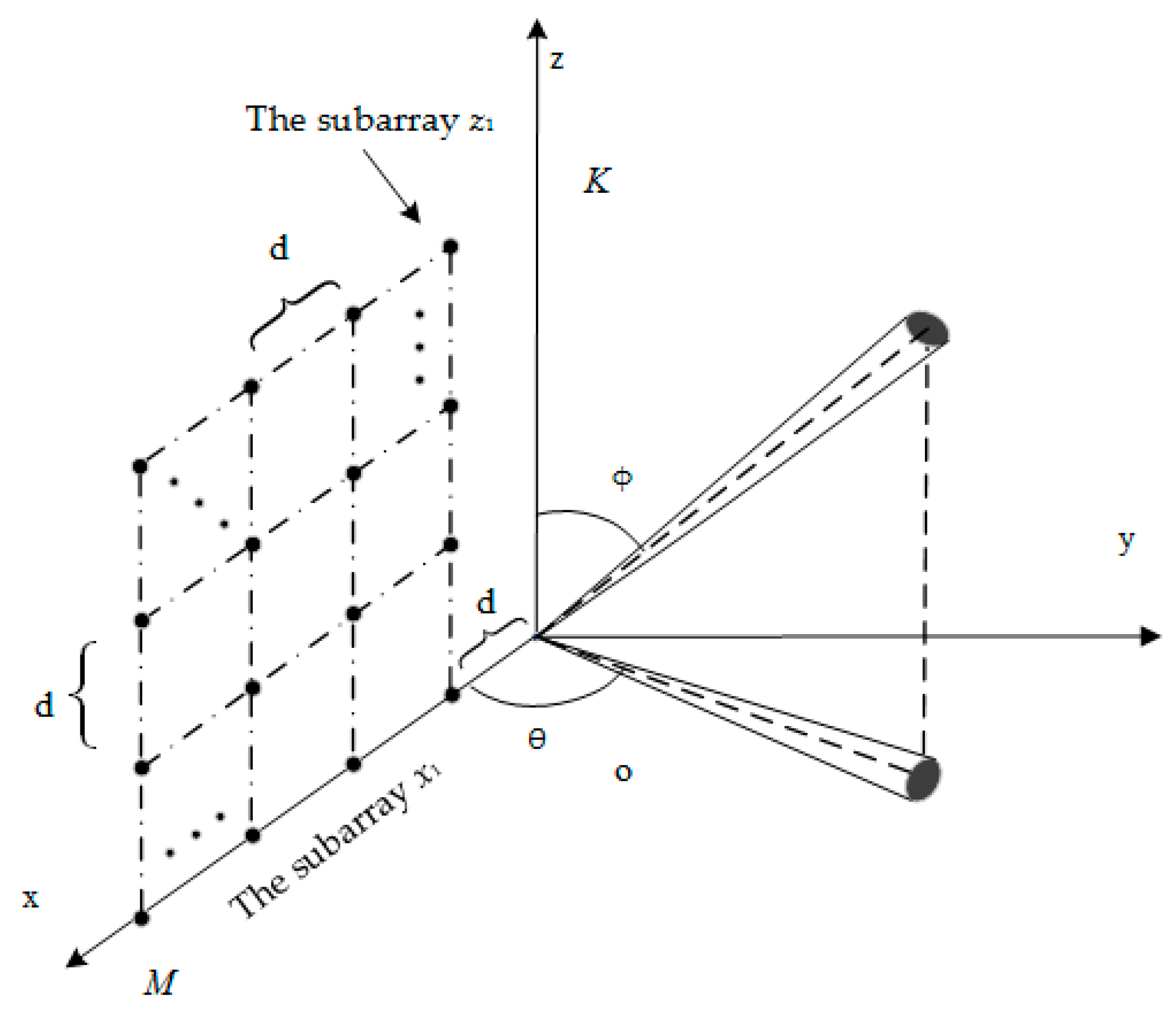
As shown in Figure 1, the URA consists of M × K sensors on xoz plane. The distance between sensors along the direction of x and z axes is set at d meters. Azimuth θ and elevation φ are used to describe the direction of signal in a three dimensional space. There are q 2D ID narrowband sources with nominal angles (θ_i, φ_i) (i = 1, 2, …, q) denoting nominal azimuth and nominal elevation of the ith sources impinging into arrays. θ_i $\in \left[0,\mathsf{\pi }\right]$, φ_i $\in \left[0,\mathsf{\pi }\right]$. λ is the wavelength of the impinging signal. The additive noise is considered as Gaussian white with zero mean and uncorrelated with sensors.

The M × 1 dimensional received vector of the M sensors located on the x-axis defined as subarray x₁ can be written as

$$x_1(t)={\displaystyle \sum _{i=1}^q{\displaystyle \iint {\mathit{\alpha }}_1(\theta ,\phi )s_i(\theta ,\phi ,t)d\theta }d\phi }+n_{x1}(t),$$

(1)

where n_x1(t) denotes the noise vector of subarray. The M × 1 dimensional vector α₁(θ,φ) denotes the steering vector of subarray x₁ with respect to point source, which can be expressed as

$${\alpha }_1(\theta ,\phi )={\left[e^{j2\pi d\cos \theta \sin \phi /\lambda },e^{j2\pi 2d\cos \theta \sin \phi /\lambda },\cdots ,e^{j2\pi Md\cos \theta \sin \phi /\lambda }\right]}^T,$$

(2)

s_i(θ,φ,t) is the complex random angular signal density of the distributed source representing the reflection intensity of the source from angle (θ,φ) at the snapshot index t. Unlike a point source, signal of a distributed source exists not only in the direction of (θ_i,φ_i) but also in a spatial distribution around (θ_i,φ_i). A distributed source is defined as incoherently distributed if s_i(θ,φ,t) from one direction is uncorrelated with other directions, which can be modeled as a random process as

$$E [s_i(\theta ,\phi ,t)s_i{}^{\ast }(\theta {}^{\prime },\phi {}^{\prime },t)]=P_i{f}_i(\theta ,\phi ;u)\delta (\theta -\theta {}^{\prime })\delta (\phi -\phi {}^{\prime }),$$

(3)

where δ(·) is the Kronecker delta function, P_i is the power of the source, f_i(θ,φ;u_i) is its normalized angular power density function (APDF) reflecting geometry and surface property of a distributed source. APDF is determined by parameter set u_i. For a Gaussian ID source, u_i = [${\theta }_i$, ${\varphi }_i$, ${\sigma }_{\theta i}$, ${\sigma }_{\varphi i}$, $\rho$] denoting nominal azimuth, nominal elevation, azimuth spread, elevation spread, and covariance coefficient respectively, APDF can be expressed as

$$f_i(\theta ,\phi ;u_i)=\frac{1}{2\pi {\sigma }_{\theta i}{\sigma }_{\phi i}\sqrt{1-{\rho }^2}}\exp \left\{-\frac{1}{2{\sigma }_{\theta i}{\sigma }_{\phi i}(1-{\rho }^2)}\left[{\left(\frac{\theta -{\theta }_i}{{\sigma }_{\theta i}}\right)}^2-2\rho \frac{(\theta -{\theta }_i)(\phi -{\phi }_i)}{{\sigma }_{\theta i}{\sigma }_{\phi i}}+{\left(\frac{\phi -{\phi }_i}{{\sigma }_{\phi i}}\right)}^2\right]\right\}$$

(4)

For a uniform ID source, u_i = [${\theta }_i$, ${\varphi }_i$, ${\sigma }_{\theta i}$, ${\sigma }_{\varphi i}$] denoting nominal azimuth, nominal elevation, azimuth spread and elevation spread respectively. APDF can be expressed as

$$f_i(\theta ,\phi ;u_i)=\{\begin{array}{ll}\frac{1}{4{\sigma }_{\theta i}{\sigma }_{\phi i}}& \left|\theta -{\theta }_i\right|\le {\sigma }_{\theta i} and \left|\phi -{\phi }_i\right|\le {\sigma }_{\phi i}\\ 0& \left|\theta -{\theta }_i\right|\ge {\sigma }_{\theta i} or \left|\phi -{\phi }_i\right|\ge {\sigma }_{\phi i}\end{array}.$$

(5)

The M × 1 dimensional received vector of the kth subarray parallel to x-axis, which is defined as subarray x_k, can be written as

$$x_k(t)={\displaystyle \sum _{i=1}^q{\displaystyle \iint {\mathit{\alpha }}_k(\theta ,\phi )s_i(\theta ,\phi ,t)d\theta }d\phi }+n_{xk}(t),$$

(6)

where α_k(θ,φ) denotes the steering vector of subarray x_k with respect to point source, which can be written as

$${\alpha }_k(\theta ,\phi )={\alpha }_1(\theta ,\phi )e^{j2\pi (k-1)d\cos \phi /\lambda }.$$

(7)

The M × K dimensional received matrix of the URA along the x-axis can be expressed as

$$X(t)={[x_1(t),x_2(t),\cdots ,x_K(t)]}^T.$$

(8)

The K × 1 dimensional received vector of the K sensors with distance d and parallel to z-axis defined as subarray z₁ can be written as

$$z_1(t)={\displaystyle \sum _{i=1}^q{\displaystyle \iint {\mathsf{\beta }}_1(\theta ,\phi )s_i(\theta ,\phi ,t)d\theta }d\phi }+n_{z1}(t),$$

(9)

where the K × 1 dimensional vector β₁(θ,φ) denotes the steering vector of subarray z₁ with respect to point source, n_z1(t) denotes the noise vector of subarray z₁. β₁(θ,φ) can be expressed as

$${\mathsf{\beta }}_1(\theta ,\phi )=e^{j2\pi d\cos \theta \sin \phi /\lambda }{\left[1,e^{j2\pi d\cos \phi /\lambda },\cdots ,e^{j2\pi (K-1)d\cos \phi /\lambda }\right]}^T.$$

(10)

The K × 1 dimensional received vector of the mth subarray parallel to z-axis defined as subarray z_m can be written as

$$z_m(t)={\displaystyle \sum _{i=1}^q{\displaystyle \iint {\mathsf{\beta }}_m(\theta ,\phi )s_i(\theta ,\phi ,t)d\theta }d\phi }+n_{zm}(t),$$

(11)

where β_m(θ,φ) denotes the steering vector of subarray z_m with respect to point source, which can be written as

$${\mathsf{\beta }}_m(\theta ,\phi )={\mathsf{\beta }}_1(\theta ,\phi )e^{j2\pi (m-1)d\cos \theta \sin \phi /\lambda }.$$

(12)

The K × M dimensional received matrix of the URA along the z-axis can be expressed as

$$Z(t)={[z_1(t),z_2(t),\cdots ,z_M(t)]}^T.$$

(13)

3. Proposed Method

This section consists of five parts. First of all, generalized steering matrices are obtained from taking the first-order Taylor series expansions of steering vectors under the assumption of small angular spreads and small distance d of the URA. Then, the rotation invariance relations of generalized steering matrices within subarrays are derived. In the next part, the received signal vectors are transformed as combinations of generalized signal vectors and generalized steering matrices. Next, based on rotation invariance relations of constructed subarrays, nominal azimuth and nominal elevation can be estimated separately by an ESPRIT like algorithm. Afterwards, angle matching method is proposed based on the Capon principle. Lastly computational procedure is summarized and complexity analysis is analyzed with comparison of two existing methods for 2D ID sources.

3.1. Generalized Steering Matrix

Assume that angular spread of distributed sources is small, take the first-order Taylor series expansions of steering vectors of subarrays x_k and x_k−1 at (θ_i, φ_i), we have

$${\alpha }_{k-1}(\theta ,\phi )\approx {\alpha }_{k-1}({\theta }_i,{\phi }_i)+[{\alpha }_{k-1}{({\theta }_i,{\phi }_i){]}^{\prime }}_{\theta }(\theta -{\theta }_i)+[{\alpha }_{k-1}{({\theta }_i,{\phi }_i){]}^{\prime }}_{\phi }(\phi -{\phi }_i),$$

(14)

$${\alpha }_k(\theta ,\phi )\approx {\alpha }_k({\theta }_i,{\phi }_i)+[{\alpha }_k{({\theta }_i,{\phi }_i){]}^{\prime }}_{\theta }(\theta -{\theta }_i)+[{\alpha }_k{({\theta }_i,{\phi }_i){]}^{\prime }}_{\phi }(\phi -{\phi }_i),$$

(15)

where ${[·{]}^{\prime }}_{\theta }$ and ${[·{]}^{\prime }}_{\phi }$ denote the first-order partial derivatives of θ and φ at (θ_i, φ_i), the following relationship can be obtained from Equation (7)

$${\alpha }_k({\theta }_i,{\phi }_i)={\alpha }_{k-1}({\theta }_i,{\phi }_i)e^{j2\pi d\cos {\phi }_i/\lambda },$$

(16)

$$[{\alpha }_k{({\theta }_i,{\phi }_i){]}^{\prime }}_{\theta }={[{\mathit{\alpha }}_{k-1}({\theta }_i,{\phi }_i){]}^{\prime }}_{\theta }{e}^{j2\pi d\cos {\phi }_i/\lambda },$$

(17)

$$[{\alpha }_k{({\theta }_i,{\phi }_i){]}^{\prime }}_{\phi }={[{\mathit{\alpha }}_{k-1}({\theta }_i,{\phi }_i){]}^{\prime }}_{\phi }{e}^{j2\pi d\cos {\phi }_i/\lambda }+(-j2\pi d\sin {\phi }_i/\lambda )e^{j2\pi (k-1)d\cos {\phi }_i/\lambda }{\alpha }_{k-1}({\theta }_i,{\phi }_i).$$

(18)

If d/λ $\ll$ 0.5, the second term of the right side of the Equation (18) can be ignored, so Equation (18) can be written as

$$[{\alpha }_k{({\theta }_i,{\phi }_i){]}^{\prime }}_{\phi }\approx {[{\mathit{\alpha }}_{k-1}({\theta }_i,{\phi }_i){]}^{\prime }}_{\phi }{e}^{j2\pi d\cos {\phi }_i/\lambda }.$$

(19)

In the point source model case, steering vectors is used to describe response of an array. Nevertheless, as for distribute sources, generalized steering vectors or generalized steering matrices [5,24] represent response of arrays. Define M × 3q dimensional generalized steering matrix of subarray x₁ as $[A_{11},A_{12},A_{13}]$. A₁₁, A₁₂, and A₁₃ are expressed as

$$\{\begin{array}{l}{A}_{11}=[{\mathit{\alpha }}_1({\theta }_1,{\phi }_1),{\mathit{\alpha }}_1({\theta }_2,{\phi }_2),\cdots ,{\mathit{\alpha }}_1({\theta }_q,{\phi }_q)]\\ A_{12}=\left[{[{\mathit{\alpha }}_1({\theta }_1,{\phi }_1){]}^{\prime }}_{\theta },{[{\mathit{\alpha }}_1({\theta }_2,{\phi }_2){]}^{\prime }}_{\theta },\cdots ,{[{\mathit{\alpha }}_1({\theta }_q,{\phi }_q){]}^{\prime }}_{\theta }\right]\\ A_{13}=\left[{[{\mathit{\alpha }}_1({\theta }_1,{\phi }_1){]}^{\prime }}_{\phi },{[{\mathit{\alpha }}_1({\theta }_2,{\phi }_2){]}^{\prime }}_{\phi },\cdots ,{[{\mathit{\alpha }}_1({\theta }_q,{\phi }_q){]}^{\prime }}_{\phi }\right]\end{array}.$$

(20)

Define the generalized steering matrix of subarray x_k as $[A_{k1},A_{k2},A_{k3}]$,

$$\{\begin{array}{l}{A}_{k1}=[{\mathit{\alpha }}_k({\theta }_1,{\phi }_1),{\mathit{\alpha }}_k({\theta }_2,{\phi }_2),\cdots ,{\mathit{\alpha }}_k({\theta }_q,{\phi }_q)]\\ A_{k2}=\left[{[{\mathit{\alpha }}_k({\theta }_1,{\phi }_1){]}^{\prime }}_{\theta },{[{\mathit{\alpha }}_k({\theta }_2,{\phi }_2){]}^{\prime }}_{\theta },\cdots ,{[{\mathit{\alpha }}_k({\theta }_q,{\phi }_q){]}^{\prime }}_{\theta }\right]\\ A_{k3}=\left[{[{\mathit{\alpha }}_k({\theta }_1,{\phi }_1){]}^{\prime }}_{\phi },{[{\mathit{\alpha }}_k({\theta }_2,{\phi }_2){]}^{\prime }}_{\phi },\cdots ,{[{\mathit{\alpha }}_k({\theta }_q,{\phi }_q){]}^{\prime }}_{\phi }\right]\end{array}.$$

(21)

From Equations (16), (17) and (19) we can obtain the generalized steering matrix of x_k subarray as

$$[A_{k1},A_{k2},A_{k3}]\approx [A_{11}{\mathsf{\Phi }}_z^{k-1},A_{12}{\mathsf{\Phi }}_z^{k-1},A_{13}{\mathsf{\Phi }}_z^{k-1}],$$

(22)

where Φ_z is rotation invariance operator, which can be written as

$${\mathsf{\Phi }}_z=diag(e^{j2\pi d\cos {\phi }_1/\lambda },e^{j2\pi d\cos {\phi }_2/\lambda },\cdots ,e^{j2\pi d\cos {\phi }_q/\lambda }).$$

(23)

Take the first-order Taylor series expansions of steering vectors of subarrays z_m and z_m−1 at (θ_i, φ_i), we have

$${\mathsf{\beta }}_{m-1}(\theta ,\phi )\approx {\mathsf{\beta }}_{m-1}({\theta }_i,{\phi }_i)+[{\mathsf{\beta }}_{m-1}{({\theta }_i,{\phi }_i){]}^{\prime }}_{\theta }(\theta -{\theta }_i)+[{\mathsf{\beta }}_{m-1}{({\theta }_i,{\phi }_i){]}^{\prime }}_{\phi }(\phi -{\phi }_i),$$

(24)

$${\mathsf{\beta }}_m(\theta ,\phi )\approx {\mathsf{\beta }}_m({\theta }_i,{\phi }_i)+[{\mathsf{\beta }}_m{({\theta }_i,{\phi }_i){]}^{\prime }}_{\theta }(\theta -{\theta }_i)+[{\mathsf{\beta }}_m{({\theta }_i,{\phi }_i){]}^{\prime }}_{\phi }(\phi -\phi ).$$

(25)

Form Equation (12) we have

$${\mathsf{\beta }}_m(\theta ,\phi )={\mathsf{\beta }}_{m-1}({\theta }_i,{\phi }_i)e^{j2\pi d\cos {\theta }_i\sin {\phi }_i/\lambda },$$

(26)

$${[{\mathsf{\beta }}_m({\theta }_i,{\phi }_i){]}^{\prime }}_{\theta }={[{\mathsf{\beta }}_{m-1}({\theta }_i,{\phi }_i){]}^{\prime }}_{\theta }{e}^{j2\pi d\cos {\theta }_i\sin {\phi }_i/\lambda }+(-j2\pi d\sin {\theta }_i\sin {\phi }_i/\lambda )e^{j2\pi d\cos {\theta }_i\sin {\phi }_i/\lambda }{\mathsf{\beta }}_{m-1}({\theta }_i,{\phi }_i),$$

(27)

$${[{\mathsf{\beta }}_m({\theta }_i,{\phi }_i){]}^{\prime }}_{\phi }={[{\mathsf{\beta }}_{m-1}({\theta }_i,{\phi }_i){]}^{\prime }}_{\phi }{e}^{j2\pi d\cos {\theta }_i\sin {\phi }_i/\lambda }+(j2\pi d\cos {\theta }_i\cos {\phi }_i/\lambda )e^{j2\pi d\cos {\theta }_i\sin {\phi }_i/\lambda }{\mathsf{\beta }}_{m-1}({\theta }_i,{\phi }_i).$$

(28)

If d/λ $\ll$ 0.5, the second term of the right side of the Equations (27) and (28) can be ignored, so Equations (27) and (28) can be written as

$${[{\mathsf{\beta }}_m({\theta }_i,{\phi }_i){]}^{\prime }}_{\theta }\approx {[{\mathsf{\beta }}_{m-1}({\theta }_i,{\phi }_i){]}^{\prime }}_{\theta }{e}^{j2\pi d\cos {\theta }_i\sin {\phi }_i/\lambda },$$

(29)

$${[{\mathsf{\beta }}_m({\theta }_i,{\phi }_i){]}^{\prime }}_{\phi }\approx {[{\mathsf{\beta }}_{m-1}({\theta }_i,{\phi }_i){]}^{\prime }}_{\phi }{e}^{j2\pi d\cos {\theta }_i\sin {\phi }_i/\lambda }.$$

(30)

Define the M × 3q dimensional generalized steering matrix of subarray z₁ as $[B_{11},B_{12},B_{13}]$; B₁₁, B₁₂, and B₁₃ are written as

$$\{\begin{array}{l}{B}_{11}=[{\mathsf{\beta }}_1({\theta }_1,{\phi }_1),{\mathsf{\beta }}_1({\theta }_2,{\phi }_2),\cdots ,{\mathsf{\beta }}_1({\theta }_q,{\phi }_q)]\\ B_{12}=\left[{[{\mathsf{\beta }}_1({\theta }_1,{\phi }_1){]}^{\prime }}_{\theta },{[{\mathsf{\beta }}_1({\theta }_2,{\phi }_2){]}^{\prime }}_{\theta },\cdots ,{[{\mathsf{\beta }}_1({\theta }_q,{\phi }_q){]}^{\prime }}_{\theta }\right]\\ B_{13}=\left[{[{\mathsf{\beta }}_1({\theta }_1,{\phi }_1){]}^{\prime }}_{\phi },{[{\mathsf{\beta }}_1({\theta }_2,{\phi }_2){]}^{\prime }}_{\phi },\cdots ,{[{\mathsf{\beta }}_1({\theta }_q,{\phi }_q){]}^{\prime }}_{\phi }\right]\end{array}.$$

(31)

Define the generalized steering matrix of subarray z₁ as $[B_{m1},B_{m2},B_{m3}]$,

$$\{\begin{array}{l}{B}_{m1}=[{\mathsf{\beta }}_m({\theta }_1,{\phi }_1),{\mathsf{\beta }}_m({\theta }_2,{\phi }_2),\cdots ,{\mathsf{\beta }}_m({\theta }_q,{\phi }_q)]\\ B_{m2}=\left[{[{\mathsf{\beta }}_m({\theta }_1,{\phi }_1){]}^{\prime }}_{\theta },{[{\mathsf{\beta }}_m({\theta }_2,{\phi }_2){]}^{\prime }}_{\theta },\cdots ,{[{\mathsf{\beta }}_m({\theta }_q,{\phi }_q){]}^{\prime }}_{\theta }\right]\\ B_{m3}=\left[{[{\mathsf{\beta }}_m({\theta }_1,{\phi }_1){]}^{\prime }}_{\phi },{[{\mathsf{\beta }}_m({\theta }_2,{\phi }_2){]}^{\prime }}_{\phi },\cdots ,{[{\mathsf{\beta }}_m({\theta }_q,{\phi }_q){]}^{\prime }}_{\phi }\right]\end{array}.$$

(32)

From Equations (26), (29), and (30), the generalized steering matrix of z_m $[B_{m1},B_{m2},B_{m3}]$ can be expressed as

$$[B_{m1},B_{m2},B_{m3}]\approx [B_{11}{\mathsf{\Phi }}_x^{m-1},B_{12}{\mathsf{\Phi }}_x^{m-1},B_{13}{\mathsf{\Phi }}_x^{m-1}],$$

(33)

where Φ_x is rotation invariance operator, which can be written as

$${\mathsf{\Phi }}_x=diag(e^{j2\pi d\cos {\theta }_1\sin {\phi }_1/\lambda },e^{j2\pi d\cos {\theta }_2\sin {\phi }_2/\lambda },\cdots ,e^{j2\pi d\cos {\theta }_q\sin {\phi }_q/\lambda }).$$

(34)

3.2. Generalized Signal Vector

Define generalized signal vector as $\overline{s}=[{\overline{s}}_1,{\overline{s}}_2,{\overline{s}}_3]$^H; ${\overline{s}}_1,{\overline{s}}_2$ and ${\overline{s}}_3$ are written as

$$\{\begin{array}{l}{\overline{s}}_1=[{\rho }_{10},{\rho }_{20},\cdots ,{\rho }_{k0}]\\ {\overline{s}}_2=[{\rho }_{1\theta },{\rho }_{2\theta },\cdots ,{\rho }_{k\theta }]\\ {\overline{s}}_3=[{\rho }_{1\phi },{\rho }_{2\phi },\cdots ,{\rho }_{k\phi }]\end{array},$$

(35)

where

$$\{\begin{array}{l}{\rho }_{i0}={\displaystyle \iint s_i(\theta ,\phi ,t)d\theta }d\phi \\ {\rho }_{i\theta }={\displaystyle \iint (\theta -{\theta }_i)s_i(\theta ,\phi ,t)d\theta }d\phi \\ {\rho }_{i\phi }={\displaystyle \iint (\phi -{\phi }_i)s_i(\theta ,\phi ,t)d\theta }d\phi \end{array}.$$

(36)

Substitute Taylor series expansions (15) into Equation (6), we obtain

$$\begin{array}{ll}{x}_k(t)& \approx {\displaystyle \sum _{i=1}^q{\displaystyle \iint {\mathit{\alpha }}_k({\theta }_i,{\phi }_i)s_i(\theta ,\phi ,t)d\theta }d\phi +}{\displaystyle \sum _{i=1}^q{\displaystyle \iint [{\mathit{\alpha }}_k{({\theta }_i,{\phi }_i){]}^{\prime }}_{\theta }(\theta -{\theta }_i)s_i(\theta ,\phi ,t)d\theta }d\phi }\\ & +{\displaystyle \sum _{i=1}^q{\displaystyle \iint [{\mathit{\alpha }}_k{({\theta }_i,{\phi }_i){]}^{\prime }}_{\phi }(\phi -{\phi }_i)s_i(\theta ,\phi ,t)d\theta }d\phi }+n_{xk}(t)\\ & ={\displaystyle \sum _{i=1}^q{\mathit{\alpha }}_k({\theta }_i,{\phi }_i){\rho }_{i0}+}{\displaystyle \sum _{i=1}^q[{\mathit{\alpha }}_k({\theta }_i,{\phi }_i){]}^{\prime }{\rho }_{i\theta }+}{\displaystyle \sum _{i=1}^q[{\mathit{\alpha }}_k{({\theta }_i,{\phi }_i){]}^{\prime }}_{\phi }{\rho }_{i\phi }}+n_{xk}(t)\end{array}$$

(37)

Thus, received vector of subarray x_k can be expressed as a combination of the generalized signal vector and generalized steering matrix

$$x_k(t)\approx [A_{k1},A_{k2},A_{k3}]\overline{s}+n_{xk}(t).$$

(38)

The MK × 1 received vector of the URA along the x-axis can be express as

$$\overline{X}(t)={[x_1{(t)}^T,x_2{(t)}^T,\cdots ,x_K{(t)}^T]}^T\approx \left[\begin{array}{ccc}{A}_{11},& A_{12},& A_{13}\\ A_{11}{\mathsf{\Phi }}_z,& A_{12}{\mathsf{\Phi }}_z,& A_{13}{\mathsf{\Phi }}_z\\ & \cdots & \\ A_{11}{\mathsf{\Phi }}_z^{K-1},& A_{12}{\mathsf{\Phi }}_z^{K-1},& A_{13}{\mathsf{\Phi }}_z^{K-1}\end{array}\right]\overline{s}+n_X(t),$$

(39)

where n_X(t) is the noise vector of the URA along the x-axis, which can be expressed as

$$n_X(t)={\left[n_{x1}{(t)}^T,n_{x2}{(t)}^T,\cdots ,n_{xK}{(t)}^T\right]}^T.$$

(40)

Similarly, the received vector of subarray z_m can be expressed as

$${\mathrm{z}}_m(t)\approx [B_{m1},B_{m2},B_{m3}]\overline{s}+n_{z1}(t).$$

(41)

Supposing different ID sources are uncorrelated there exist following relations within generalized signal vectors (see Appendix A)

$$E[{\rho }_{il}{\rho }_{in}^{\ast }]=\{\begin{array}{ll}{P}_i& l=n=0\\ P_i{M}_{\theta i}& l=n=\theta \\ P_i{M}_{\phi i}& l=n=\phi \\ 0& l\ne \mathrm{n}\end{array},$$

(42)

where M_θi, M_φi can be express as

$$M_{\theta i}={\displaystyle \iint {(\theta -{\theta }_i)}^2{p}_i(\theta ,\phi ,t)d\theta }d\phi ,$$

(43)

$$M_{\phi i}={\displaystyle \iint {(\phi -{\phi }_i)}^2{p}_i(\theta ,\phi ,t)d\theta }d\phi .$$

(44)

According to the assumption that different ID sources are uncorrelated, so we have

$$E [\overline{s}{\overline{s}}^H]=diag(\Lambda ,M_{\theta }\Lambda ,M_{\phi }\Lambda ),$$

(45)

where Λ, M_θ, and M_φ can be written as

$$\{\begin{array}{l}\Lambda =diag({\sigma }_{s1}^2,{\sigma }_{s2}^2,\cdots ,{\sigma }_{sq}^2)\\ M_{\theta }=diag(M_{\theta 1},M_{\theta 2},\cdots ,M_{\theta q})\\ M_{\phi }=diag(M_{\phi 1},M_{\phi 2},\cdots ,M_{\phi q})\end{array}.$$

(46)

3.3. Nominal Angles Estimation

We construct two subarrays X₁ and X₂ along the direction of the x-axis. X₁ is constituted by arrays from x₁ to x_K−1; while X₂ contains arrays from x₂ to x_K. Thus, X₁(t) is M(K − 1) × 1 dimensional received vector of X₁ also equals a vector containing elements from 1 to MK − M row of $\overline{X}$(t); whereas X₂(t) is M(K − 1) × 1 dimensional received vector of X₂ containing elements from M + 1 to MK of $\overline{X}$(t). X₁(t) and X₂(t) can be written as

$$\{\begin{array}{l}{X}_1(t)={[x_1{(t)}^T,x_2{(t)}^T,\cdots ,x_{K-1}{(t)}^T]}^T=\left[A_{x1}^1,A_{x2}^1,A_{x3}^1\right]\overline{s}+n_{X1}(t)\\ X_2(t)={[x_2{(t)}^T,x_2{(t)}^T,\cdots ,x_K{(t)}^T]}^T=\left[A_{x1}^2,A_{x2}^2,A_{x3}^2\right]\overline{s}+n_{X2}(t)\end{array},$$

(47)

n_X1(t) is noise vector of X₁ containing elements from 1 to MK − M row of n_X(t), n_X2(t) is noise vector of X₂ containing elements from M to MK row of n_X(t). $\left[A_{x1}^1,A_{x2}^1,A_{x3}^1\right]$ is the generalized steering matrix of subarray X₁(t), which can be expressed as

$$\left[A_{x1}^1,A_{x2}^1,A_{x3}^1\right]=\left[\begin{array}{ccc}{A}_{11},& A_{12},& A_{13}\\ A_{11}{\mathsf{\Phi }}_z,& A_{12}{\mathsf{\Phi }}_z,& A_{13}{\mathsf{\Phi }}_z\\ & \cdots & \\ A_{11}{\mathsf{\Phi }}_z^{K-2},& A_{12}{\mathsf{\Phi }}_z^{K-2},& A_{13}{\mathsf{\Phi }}_z^{K-2}\end{array}\right],$$

(48)

$\left[A_{x1}^2,A_{x2}^2,A_{x3}^2\right]$ is the generalized steering matrix of subarray X₂(t). From Equation (22) we can obtain

$$\left[A_{x1}^2,A_{x2}^2,A_{x3}^2\right]\approx \left[A_{x1}^1{\mathsf{\Phi }}_z,A_{x2}^1{\mathsf{\Phi }}_z,A_{x3}^1{\mathsf{\Phi }}_z\right],$$

(49)

which proves the rotational invariance relation between the two constructed subarrays X₁ and X₂. According to the ESPRIT principle, combing the vector X₁(t) and X₂(t), we obtain a vector with rotational invariance property as

$$X_{12}(t)=\left[\begin{array}{l}{X}_1(t)\\ X_2(t)\end{array}\right]=\left[A_{x1},A_{x2},A_{x3}\right]\overline{s}+n_{X12}(t),$$

(50)

where the generalized steering matrix of the combination X₁₂(t) can be expressed as

$$\left[A_{x1},A_{x2},A_{x3}\right]=\left[\begin{array}{l}{A}_{x1}^1,A_{x2}^1,A_{x3}^1\\ A_{x1}^2,A_{x2}^2,A_{x3}^2\end{array}\right].$$

(51)

The combination of noise vector can be expressed as

$$n_{X12}(t)=\left[\begin{array}{l}{n}_{X1}(t)\\ n_{X2}(t)\end{array}\right].$$

(52)

ESPRIT framework is based on rotational invariance property of signal subspace, which can be derived from the rotational invariance property of the received signal vector. Signal subspace can be acquired by eigendecomposition of the covariance matrix of received vector X₁₂(t) which can be expressed as

$$R_{\mathrm{x}}^{12}=E [X_{12}(\mathrm{t})X_{12}^H(\mathrm{t})].$$

(53)

$R_x^{12}$ can be replaced by sample covariance matrix with N snapshots as

$${\widehat{R}}_x^{12}=\frac{1}{N}{\displaystyle \sum _{t=1}^N{X}_{12}(t)X_{12}^H(t)}.$$

(54)

From Equations (45) and (46) we find that eigenvalues of covariance matrix of received signal vector consist of three parts Λ, M_θΛ and M_φΛ. The three parts all has q elements. Each part corresponds to respective eigenvectors. Under the assumption of small angular spread, we can obtain M_θi < 1 and M_φi < 1. Therefore, subspace spanned by eigenvectors corresponding to the largest q eigenvalues is equal to subspace spanned by A_x1. Suppose E_x is 2M(K − 1) × q dimensional matrix with columns as the eigenvectors of the covariance matrix $R_x^{12}$ corresponding to the q largest eigenvalues. Accordingly, there exists a q × q nonsingular matrix T satisfying the following relation

$$E_x=\left[\begin{array}{l}{A}_{x1}^1\\ A_{x1}^1{\mathsf{\Phi }}_z\end{array}\right]T.$$

(55)

Let E_x1 and E_x2 denote matrices selecting upper and lower MK − M rows of E_x

$$\{\begin{array}{l}{E}_{x1}=A_{x1}^{1}T\\ E_{x2}=A_{x1}^{2}T\end{array}.$$

(56)

So we have

$$E_{x2}=E_{x1}T{ }^{-1}{\mathsf{\Phi }}_{z}T.$$

(57)

Let

$${\Omega }_x=T{ }^{-1}{\mathsf{\Phi }}_{z}T.$$

(58)

Thus, the eigenvalues of Φ_x is elements of Ф_z. Ω_x can be obtained as

$${\Omega }_x=E_{x1}^{+}{E}_{x2},$$

(59)

where (•)⁺ denotes pseudo-inverse operator, then the nominal elevation of the sources can be get from

$${\phi }_i=\arccos \frac{angle({\eta }_i)}{2\pi d/\lambda }i=1,2,\cdots ,q,$$

(60)

where η_i is the ith eigenvalues of Ω_x, angle(•) denotes argument of complex variable.

Similarly, we construct two subarrays Z₁ and Z₂ along the direction of z-axis. Z₁ is constituted by arrays from z₁ to z_M−1; while Z₂ contains arrays from z₂ to z_M.$Z$₁(t) is K(M − 1) × 1 dimensional receive vector of Z₁ containing elements from 1 to K(M − 1) row of $\overline{Z}$(t); whereas Z₂(t) is K(M − 1) × 1 dimensional received vector of Z₂ containing elements from K + 1 to MK row of $\overline{Z}$(t). n_Z1(t) and n_Z2(t) have the similar definition as n_X1(t) and n_X2(t). The received vectors Z₁(t) and Z₂(t) can be expressed as

$$\{\begin{array}{l}{Z}_1(t)={[z_1{(t)}^T,z_2{(t)}^T,\cdots ,z_{M-1}{(t)}^T]}^T=\left[B_{z1}^1,B_{z2}^1,B_{z3}^1\right]\overline{s}+n_{Z1}(t)\\ Z_2(t)={[z_2{(t)}^T,z_2{(t)}^T,\cdots ,z_M{(t)}^T]}^T=\left[B_{z1}^2,B_{z2}^2,B_{z3}^2\right]\overline{s}+n_{Z2}(t)\end{array},$$

(61)

where $\left[B_{z1}^1,B_{z2}^1,B_{z3}^1\right]$ is the generalized steering matrix of Z₁(t), which can be expressed as

$$\left[B_{z1}^1,B_{z2}^1,B_{z3}^1\right]=\left[\begin{array}{ccc}{B}_{11},& B_{12},& B_{13}\\ B_{11}{\mathsf{\Phi }}_x,& B_{12}{\mathsf{\Phi }}_x,& B_{13}{\mathsf{\Phi }}_x\\ & \cdots & \\ B_{11}{\mathsf{\Phi }}_x^{M-2},& B_{12}{\mathsf{\Phi }}_x^{M-2},& B_{13}{\mathsf{\Phi }}_x^{M-2}\end{array}\right].$$

(62)

Form Equation (33), the generalized steering matrix of Z₂(t) $\left[B_{z1}^2,B_{z2}^2,B_{z3}^2\right]$ can be obtained as

$$\left[B_{z1}^2,B_{z2}^2,B_{z3}^2\right]\approx \left[B_{z1}^1{\mathsf{\Phi }}_x,B_{z2}^1{\mathsf{\Phi }}_x,B_{z3}^1{\mathsf{\Phi }}_x\right],$$

(63)

which proves the rotational invariance relation between the two constructed subarrays Z₁ and Z₂. Combing the vector Z₁(t) and Z₂(t), we obtain a vector with rotational invariance property as

$$Z_{12}(t)=\left[\begin{array}{l}{Z}_1(t)\\ Z_2(t)\end{array}\right]=\left[{{\rm B}}_{z1},{{\rm B}}_{z2},{{\rm B}}_{z3}\right]\overline{s}+n_{Z12}(t),$$

(64)

where the generalized steering matrix of Z₁₂(t) can be expressed as

$$\left[{{\rm B}}_{z1},{{\rm B}}_{z2},{{\rm B}}_{z3}\right]=\left[\begin{array}{l}{B}_{z1}^1,B_{z2}^1,B_{z3}^1\\ B_{z1}^2,B_{z2}^2,B_{z3}^2\end{array}\right].$$

(65)

The combination of noise vector of Z₁(t) and Z₂(t) can be expressed as

$$n_{Z12}(t)=\left[\begin{array}{l}{n}_{Z1}(t)\\ n_{Z2}(t)\end{array}\right].$$

(66)

The covariance matrices of received signal Z₁₂(t) can be expressed as

$$R_z^{12}=E[Z_{12}(t)Z_{12}^H(t)].$$

(67)

which can be replaced by sample covariance matrix with N snapshots as

$${\widehat{R}}_z^{12}=\frac{1}{N}{\displaystyle \sum _{t=1}^N{Z}_{12}(t)Z_{12}^H(t)}.$$

(68)

Suppose E_z is 2K(M − 1) × q matrix with columns as the eigenvectors of the covariance matrix $R_z^{12}$ corresponding to the q largest eigenvalues. As the same as E_x, E_z is the same subspace spanned by $B_{z1}$. Accordingly, there exists a q × q nonsingular matrix Q satisfying the following relation

$$E_z=\left[\begin{array}{l}{B}_{11}\\ B_{11}{\mathsf{\Phi }}_x\end{array}\right]Q.$$

(69)

Let E_z1 and E_z2 denote matrices selecting upper and lower MK − K rows of E_z

$$\{\begin{array}{l}{E}_{z1}=B_{z1}^{1}Q\\ E_{z2}=B_{z1}^{1}Q\end{array}.$$

(70)

So we have

$$E_{\mathrm{z}2}=E_{\mathrm{z}1}{Q}^{-1}{\mathsf{\Phi }}_{\mathrm{x}}Q.$$

(71)

Let

$${\Omega }_z=Q^{-1}{\mathsf{\Phi }}_{x}Q.$$

(72)

Thus, the eigenvalues of Φ_z is elements of Ф_x. Ω_z can be obtained as

$${\Omega }_z=E_{z1}^{+}{E}_{z2}.$$

(73)

Then the nominal azimuth of the sources can be get from

$${\theta }_i=\arccos \frac{angle({\mu }_i)}{2\pi d/\lambda \sin {\phi }_i}i=1,2,\cdots ,q,$$

(74)

where μ_i is the ith eigenvalues of Ω_z.

3.4. Angle Matching Method

After all the eigenvalues of Ω_x and Ω_z are calculated, we need to match the right θ_i to right φ_i. We can obtain cost function by applying Capon principle to subarray x₁ firstly. Then angle matching can be obtained by substituting all the possible pairs into the cost function.

The generalized steering matrix of subarray x₁ is $\left[A_{11},A_{12},A_{13}\right]$, the Capon principle with regard to the subarray x₁ can be expressed as

$$\min w^H{R}_x^{1}w subject to w^H\left[A_{11},A_{12},A_{13}\right]=1.$$

(75)

where $R_x^1$ is the covariance matrix of subarray x₁. Equation (75) can be solved through minimization of Lagrange function as follows

$$L(\theta ,\phi )=w^H{R}_x^{1}w +\lambda \left\{w^H\left[A_{11},A_{12},A_{13}\right]-1\right\},$$

(76)

Take the derivative of the Equation (76) with regard to w and set the result equal to 0, we obtain

$$R_x^{1}w =-\left[A_{11},A_{12},A_{13}\right]\lambda ,$$

(77)

Considering constraint condition, we obtain

$$\lambda =-{\left\{{\left[A_{11},A_{12},A_{13}\right]}^H{(R_x^1)}^{-1}\left[A_{11},A_{12},A_{13}\right]\right\}}^{-1},$$

(78)

The optimal vector w_opt can be obtained as follows

$$w_{opt}=-\frac{{(R_x^1)}^{-1}\left[A_{11},A_{12},A_{13}\right]}{{\left[A_{11},A_{12},A_{13}\right]}^H{(R_x^1)}^{-1}\left[A_{11},A_{12},A_{13}\right]},$$

(79)

Then, the cost function can be expressed as

$$V(\theta ,\phi )=\frac{1}{{\left[A_{11},A_{12},A_{13}\right]}^H{(R_x^1)}^{-1}\left[A_{11},A_{12},A_{13}\right]}.$$

(80)

$R_x^1$ can be replaced by sample covariance matrix with N snapshots as

$${\widehat{R}}_x^1=\frac{1}{N}{\displaystyle \sum _{t=1}^N{x}_1(t)x_1^H(t)}.$$

(81)

Suppose that all eigenvalues of Ω_x and Ω_z are calculated. Now we summarize the angle matching procedure as follows:

Step 1: Calculate nominal elevation φ_i (i = 1, 2,…, q) from Equation (60). Select one elevation angle ${\widehat{\phi }}_i={\phi }_i$ form set $\{{\phi }_1,{\phi }_2,\cdots ,{\phi }_q\}$ at random. Superscript _^ denotes the angle already determined. Substitute ${\widehat{\phi }}_i$ to the eigenvalues set of Ω_z:$\{angle({\mu }_1),angle({\mu }_2),\cdots ,angle({\mu }_q)\}$ and calculate q matching azimuth angles ${\theta }_j$ $(j=1,2,\cdots ,q)$ from Equation (74). So we get q possible pairs $({\theta }_j,{\widehat{\phi }}_i)$ $(j=1,2,\cdots ,q)$.

Step 2: As the right parameters of sources can meet the objective function in Equation (75). Substitute $({\theta }_j,{\widehat{\phi }}_i)$ $(j=1,2,\cdots ,q)$ into cost function (80). Choose the azimuth ${\theta }_j$ making $V({\theta }_j,{\widehat{\phi }}_i)$ reach the maximum as the right azimuth angle matching to ${\widehat{\phi }}_i$, which is labeled as ${\widehat{\theta }}_i$.

Step 3: Delete ${\widehat{\phi }}_i$ from set $\{{\phi }_1,{\phi }_2,\cdots ,{\phi }_q\}$ meanwhile delete eigenvalue $e^{j2\pi d/\lambda \cos {\widehat{\theta }}_i\sin {\widehat{\phi }}_i}$ from set $\{angle({\mu }_1),angle({\mu }_2),\cdots ,$ $angle({\mu }_q)\}$.

Step 4: Set q = q − 1.

Step 5: Repeat steps 1 to 4.

All the nominal azimuth and nominal elevation can be matched after (q + 2)(q − 1)/2 times calculation.

3.5. Computational Procedure and Complexity Analysis

Now, our algorithm can be summarized as follows

Step 1: Compute sample covariance matrices ${\widehat{R}}_x^{12}$ and ${\widehat{R}}_z^{12}$ using Equations (54) and (68).

Step 2: Find the eigenvectors E_x and E_z corresponding to the q largest eigenvalues through eigendecomposition of ${\widehat{R}}_x^{12}$ and ${\widehat{R}}_z^{12}$. Divide E_x into E_x1, E_x2 and divide E_z into E_z1, E_z2.

Step 3: Obtain Ω_x and Ω_z from Equations (59) and (73), calculate eigenvalues ${\mu }_i$ and ${\eta }_i$ (i = 1, 2, …, q) through eigendecomposition of Ω_x and Ω_z.

Step 4: Calculate nominal azimuth θ_i and nominal elevation φ_i from Equations (60) and (74).

Step 5: Compute sample covariance matrix ${\widehat{R}}_x^1$ form Equation (81) and take the angle matching procedure.

We analyze the computational complexity of the proposed method in comparison with COMET [23] which can be applied for URA and Zhou’s algorithm [24] which uses DPULA for 2D ID sources. COMET [23] is a method under alternating projection algorithm framework, its computational cost mostly consists of the calculation of the sample covariance matrix which needs O(NM²K²) and the alternating projection technique with respect to cost functions which is O(M⁴K⁴ + 2M²K²). Zhou’s algorithm uses TLS-ESPRIT to calculate nominal elevation and 1D searching to find nominal azimuth. Computational cost of Zhou’s algorithm [24] mainly contains calculation of the sample covariance matrix O(4NM²), eigendecomposition and inversion of the sample covariance matrix O(16M³) and 1D searching O(8M³). Computational cost of the proposed algorithm mainly contains calculation of the sample covariance matrix O[N(MK − K)² + N(MK − M)²], eigendecomposition of ${\widehat{R}}_x^{12}$ and ${\widehat{R}}_z^{12}$ O[8 (MK − K)³ + 8(MK − M)³], eigendecomposition of Ω_x and Ω_z O(q³) and angle matching O(q²). The main computational complexity of the three algorithms are shown in

Table 1. Computational complexity of different methods

Method	Total
COMET algorithm [23]	O(NM2K2) + O(M4K4 + 2M2K2)
Zhou’s algorithm [24]	O(4NM2) + O(16M3) + O(8M3)
Proposed algorithm	O[N(MK − K)2 + N(MK − M)2] + O[8(MK − K)3 + 8(MK − M)3] + O(q3) + O(q2)

.

From Table 1, we can conclude that the computational cost of the proposed algorithm is higher than Zhou’s algorithm [24] when K > 2 and lower than COMET algorithm [23] when the two algorithm use same number of sensors.

4. Results and Discussion

In this section, the effectiveness of the proposed algorithm is investigated through five simulation experiments. The array configuration is shown in Figure 1. Root mean squared error (RMSE) is applied for the evaluation of the performance of estimation. RMSE_θ and RMSE_φ denote the RMSE of nominal azimuth and nominal elevation respectively, which can be expressed as

$$RMS{E}_{\theta }=\sqrt{\frac{1}{Mc}{\displaystyle \sum _{\varsigma }^{Mc}{({\widehat{\theta }}^{\varsigma }-\theta )}^2}},$$

(82)

$$RMS{E}_{\phi }=\sqrt{\frac{1}{Mc}{\displaystyle \sum _{\varsigma }^{Mc}{({\widehat{\phi }}^{\varsigma }-\phi )}^2}},$$

(83)

where MC is the number of Monte Carlo simulations. ${\widehat{\theta }}_i^{\varsigma }$ and ${\widehat{\phi }}_i^{\varsigma }$ are the estimated nominal azimuth and nominal elevation of ith source in $\varsigma$th Monte Carlo simulation.

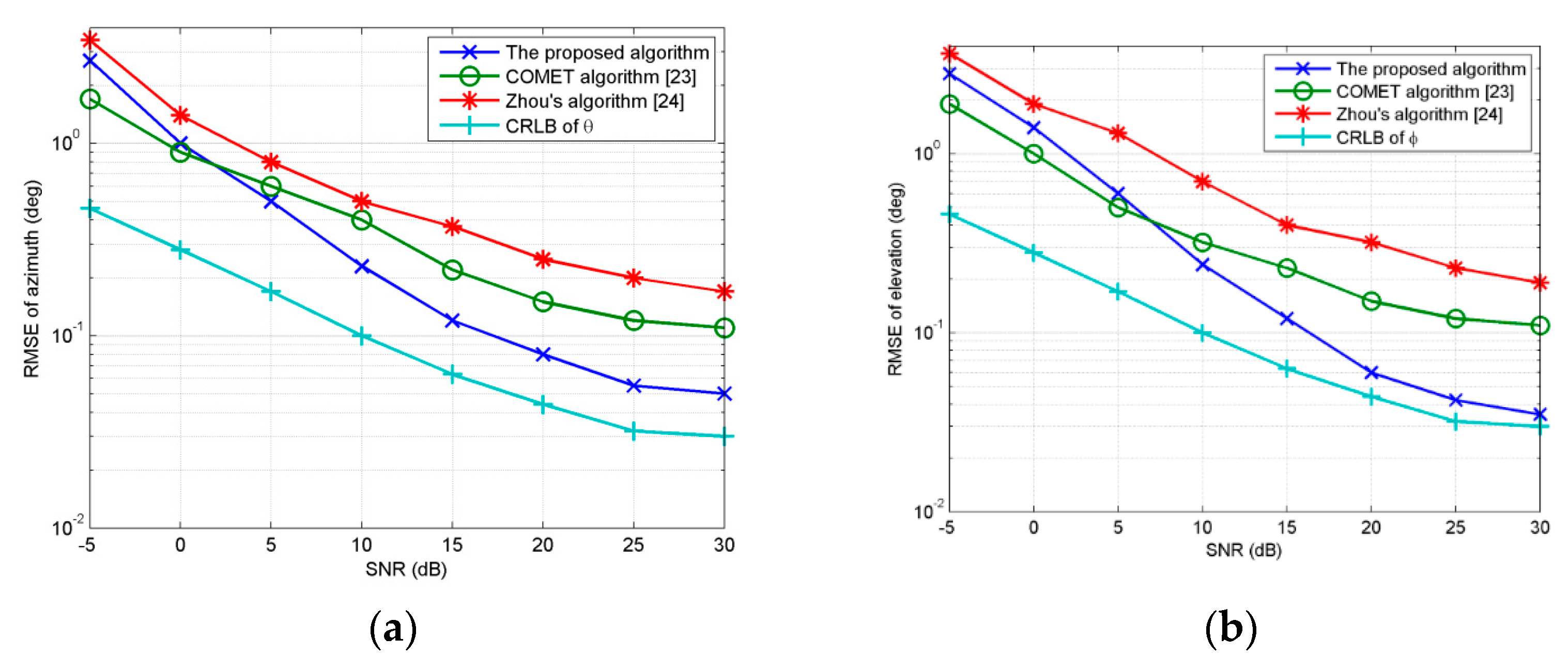
In the first experiment, we examine the performance of the proposed method vesus SNR with regard to two Gaussian ID source with parameters [30°, 45°, 2°, 2°, 0.5] and [50°, 45°, 2°, 2°, 0.5]. The sources are supposed to have the same power. Snapshots number is set at 200, MC = 100, M = K = 8. d = λ/10. Figure 2a,b show RMSE_θ and RMSE_φ curves with SNR varying from −5 dB to 30 dB. The figures also show the estimation of the COMET [23] using the URA, Zhou’s algorithm [24] using arrays x₁ and x₂ and the Cramer–Rao lower bound (CRLB). As shown from Figure 2a,b, when SNR changes from −5 dB to 0 dB, COMET [23] presents better performance than the proposed algorithm. As SNR increases, RMSE_θ and RMSE_φ of all algorithms decrease. The proposed algorithm has better performance than other algorithms with SNR ranging from 10 dB to 30 dB. Thus, it can be concluded that our method has a good performance when SNR is at high levels. Estimation of our method is based on acquiring signal subspace through eigendecomposition of covariance matrix of received vector. 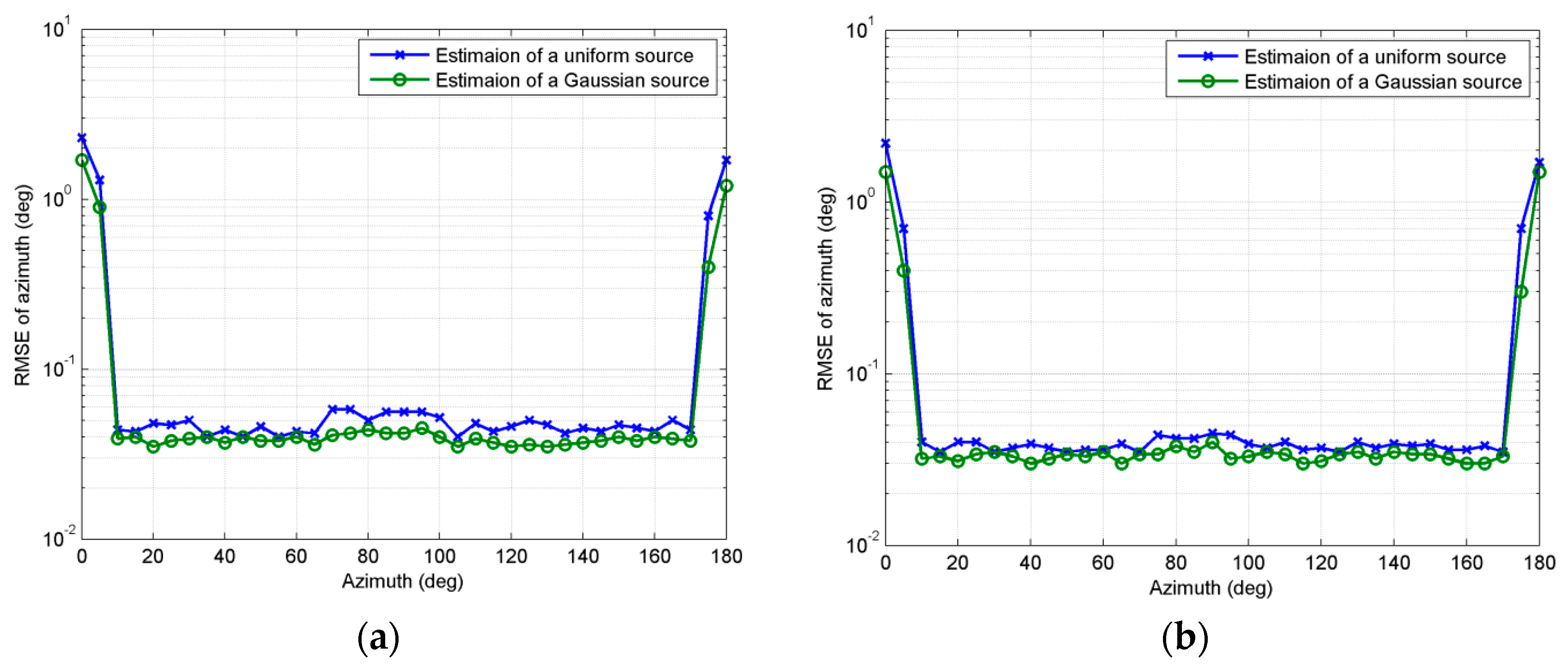The accuracy of eigendecomposition would deteriorate at low SNR, while COMET [23] separates the noise and signal power through covariance matching fitting matrix by alternating projection technique firstly, as a result, perform better at low SNR.

In the second experiment, we investigate the estimation of source near the boundary region. Consider a Gaussian and a uniform ID source respectively. Both sources have angular spread ${\sigma }_{\mathsf{\theta }}={\sigma }_{\varphi }=$2°. Covariance coefficients of Gaussian sources are set at 0.5. SNR is set at 15 dB and snapshots number is 200, MC = 100, M = K = 8, d = λ/10. Figure 3a shows RMSE_θ curves as nominal azimuth changing from 0° to 180° with nominal elevation fixed at 20°, while Figure 3b shows RMSE_φ curves as nominal elevation changing from 0° to 180° with nominal azimuth fixed at 20°. As can be seen, both RMSE_θ and RMSE_φ increase markedly near the boundary region. Generally, the error of the boundary region estimated by our method is acceptable.

In the third experiment, we examine the performance of the proposed method with regard to estimation of sources with different APDFs simultaneously. Consider four ID sources with same power and parameters of sources are set as [30°, 45°, 2°, 2°, 0.5], [50°, 45°, 1.5°, 3°, 0.5], [50°, 60°, 2°, 2.5°], and [70°, 60°, 1.5°, 3.5°]. The first and second sources are Gaussian whereas the third and fourth sources are uniform. The experiment set SNR at 15 dB; number of snapshots is 200. MC = 100, M = K = 8, d = λ/10. Figure 4 shows the estimated result of four sources, which indicate that the proposed method can estimate sources with different APDFs effectively.

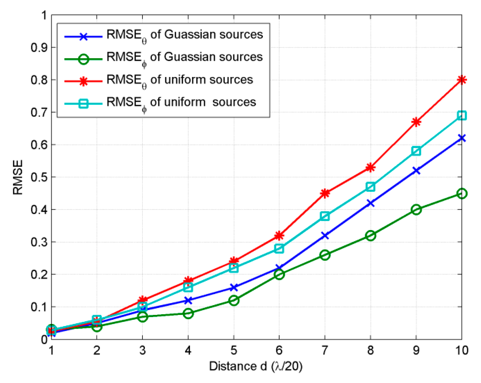
In the fourth experiment, we examine the performance of the proposed method vesus the distance d between adjacent sensors. As the rotational invariance relations of generalize steering matrices are obtained under the small distance d assumption, it is necessary to investigate the influence of d to the estimation. Four sources with the same parameters as the sources in third example are set to be estimated as the d varying from λ/20 to λ/2. SNR is set at 15 dB and snapshots number is 200, MC = 100, M = K = 8. Figure 5 shows that RMSE_θ and RMSE_φ of both Gaussian and uniform sources increase with the distance d from λ/20 to λ/2. When d is λ/2, RMSE_θ and RMSE_φ of Gaussian sources reach 0.62 and 0.44, those of uniform sources reach 0.79 and 0.67, which are still satisfactory results. It can be concluded that the proposed algorithm shows satisfactory performance with small distance between adjacent sensors.

According to the result of third example, the smaller distance d is, the higher estimation accuracy is. However, in the same channel the frequency increases, wavelength decreases. High frequency detection needs smaller d than low frequency detection to attain the same estimation accuracy. Actually, when the distance d is small, installation accuracy of sensors will get worse, which would also deteriorate the estimation accuracy. Thus, installation accuracy and the distance d is a matter of balance especially in high frequency detection. In the field of low frequency underwater detection, frequency of sonar can be down to 100 HZ, which means wavelength can reach 14.5 m approximately, on this condition d/λ can reach a small value practically.

In the fifth experiment, we investigate the performance of the proposed algorithm versus the number of sources and sensors. Theoretically, if M = K, the proposed algorithm can estimate M(M − 1) different ID sources and COMET [23] can estimate M². Utilizing double parallel arrays which contains only 2M sensors can estimate M sources simultaneously. We consider seven URA with M varying from 4 to 10. The total number of sources is set at M² which is a theoretical upper limit of the trail. The (a, b)th source is set at [20° + (a − 1)10°, 20° + (b − 1)10°]. All sources are Gaussian and have same power. SNR is 15 dB, number of snapshots is 200, MC = 100, d = λ/10, ${\sigma }_{\theta }={\sigma }_{\varphi }=$2°. Covariance coefficients of Gaussian sources are set at 0.5. When all sources are estimated successfully, the difference between estimators is accuracy which can be described by RMSE. When not all sources are estimated successfully, RMSE cannot differentiate performance of estimators. Thus, an indicator reflecting the number of sources detected is needed to measure the performance of different estimators. Estimation is regarded as effective when the estimated angles satisfying $\sqrt{{({\widehat{\theta }}_i-{\theta }_i)}^2+{({\widehat{\phi }}_i-{\phi }_i)}^2}\le$ 5°. Define detection probability as N_d/M² where N_d is number of source estimated effectively. So in theory the detection probability of the proposed algorithm is (M − 1)/M, COMET is 1, Zhou’s algorithm [24] is 1/M.

As can be seen from Figure 6, the estimation probability of zhou’s algorithm [24] is consistent with theoretical value within all range of the trail, so are the estimation probabilities of our method and COMET with M < 6. When M ≥ 7, our method perform better than COMET, which means using 7 × 7 or larger arrays our method can estimated more sources than COMET if there are large number of sources that need estimating Involving eigendecomposition of high dimensional matrices, effectiveness of our method deteriorates as the number of sources becomes large. For instance, if M = 8 and total source is 64, the covariance matrix of received vector $R_z^{12}$ is 112 × 112 dimensional, Ω_x and Ω_z is 64 × 64 dimensional, which all need eigendecomposition. The deterioration of COMET [23] is also closely related to the number of sources. COMET [23] separates unknown variables of each source based on alternating projection technique, and then formulate equation sets of unknown variables. In the separating process, 64 inversion operations of a 64 × 64 dimensional matrix are executed on the condition M = 8 and total source is 64. Consequently, the errors of the separating process deliver to equations set and affect the validity of estimation.

5. Conclusions

In this paper, we propose an estimator for 2D ID sources using URA. The received signal vectors can be transformed as combinations of generalized signal vectors and generalized steering matrices through Taylor series expansions. By virtue of the rotational invariance relations of generalized steering matrices within subarrays, an ESPRIT like algorithm are introduced in detail, then angle matching method based on Capon principle is proposed. Simulations demonstrate the effectiveness of the proposed method with regard to sources with different APDF, distance d between sensors, sources in boundary region. Simulation also indicates that our method has better performance when SNR is at high level on the condition that the quantity of sources is relatively small and can estimate more sources in sufficient sources circumstance using large dimensional arrays.