
Measuring Dynamic Signals with Direct Sensor-to-Microcontroller Interfaces Applied to a Magnetoresistive Sensor


Abstract
:1. Introduction
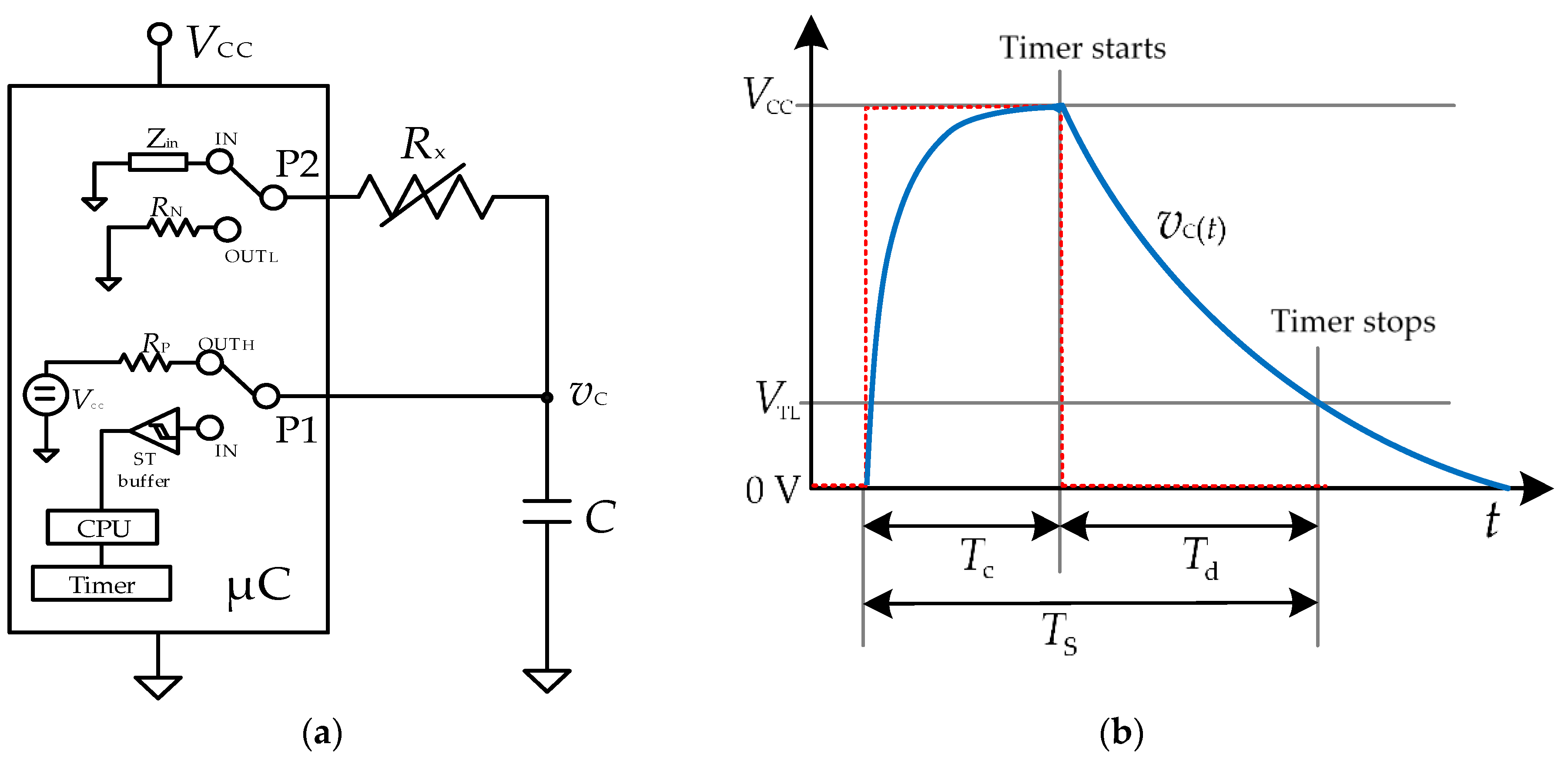
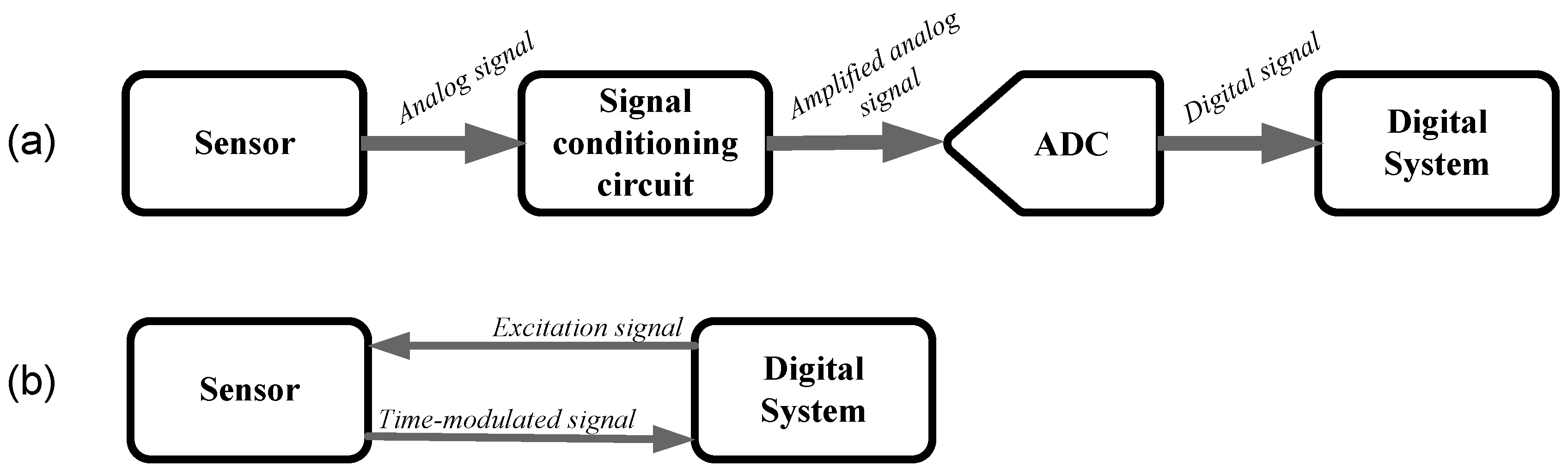
2. Operating Principle
3. Analysis of the Dynamic Performance
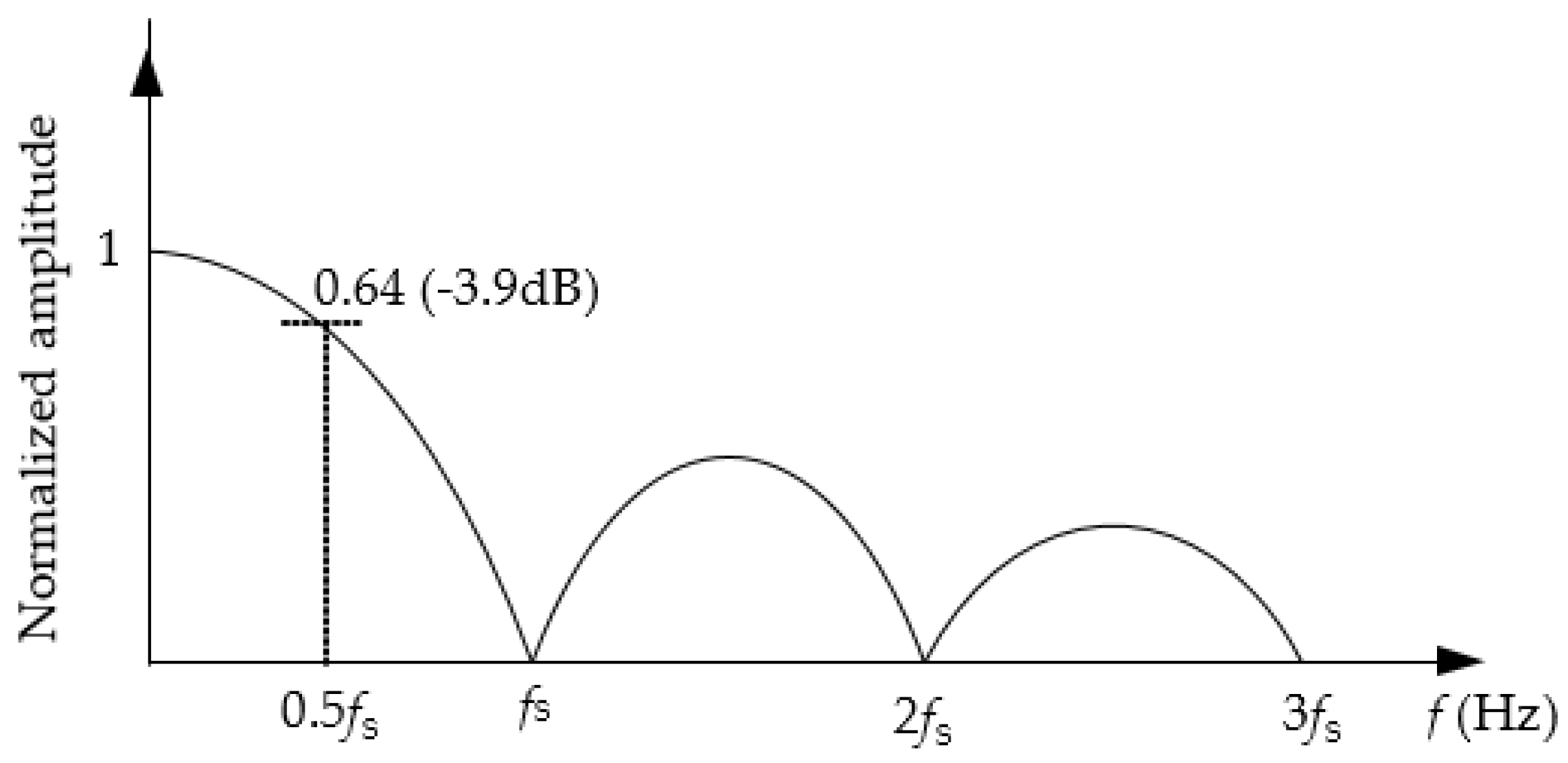
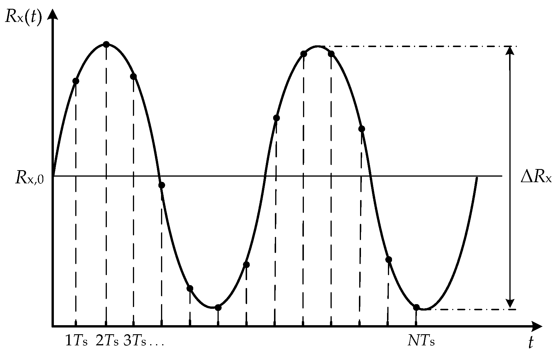
3.1. Sampling Frequency
3.2. Frequency Response
3.3. Resolution
3.4. Trade-Offs
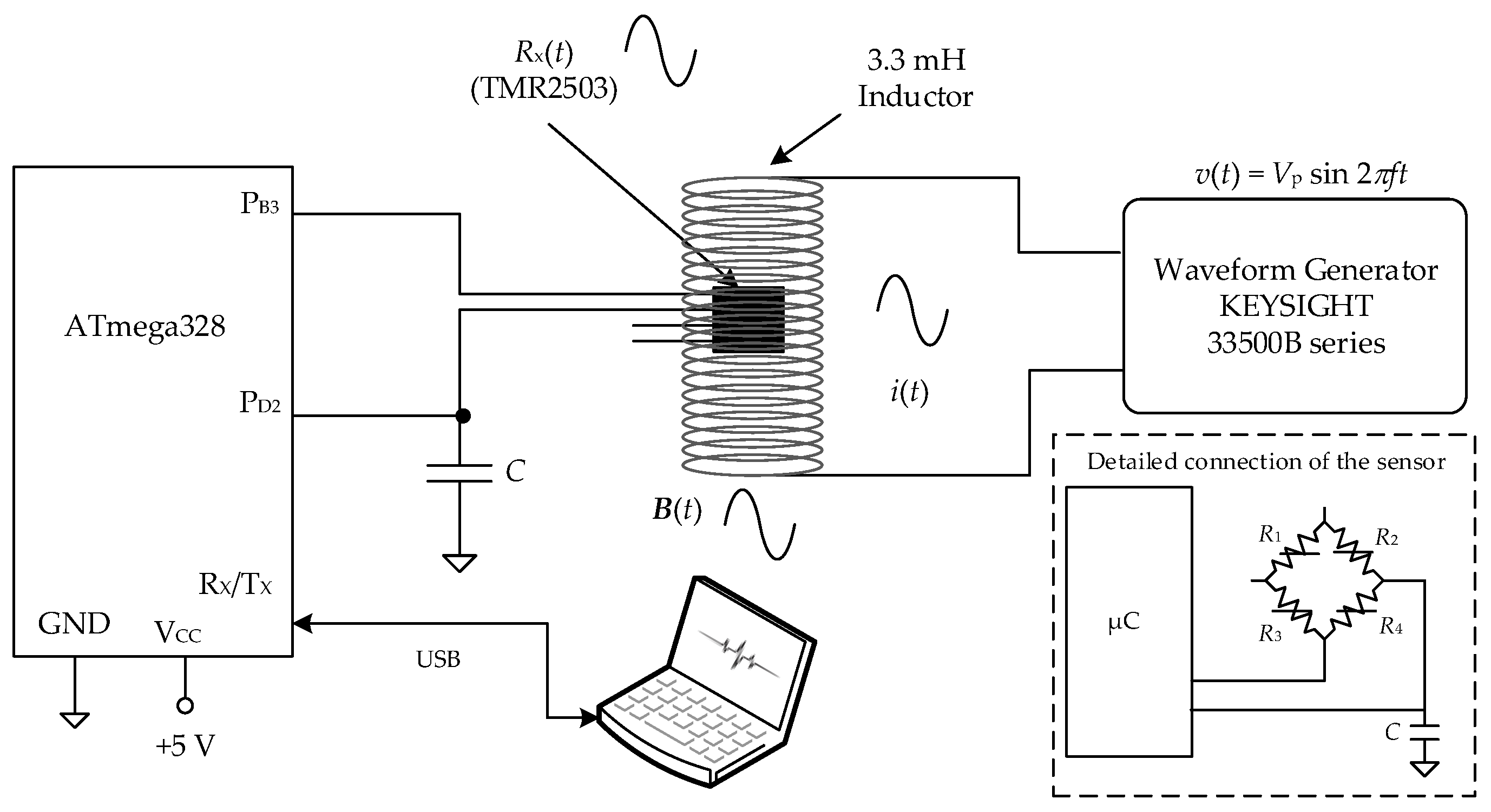
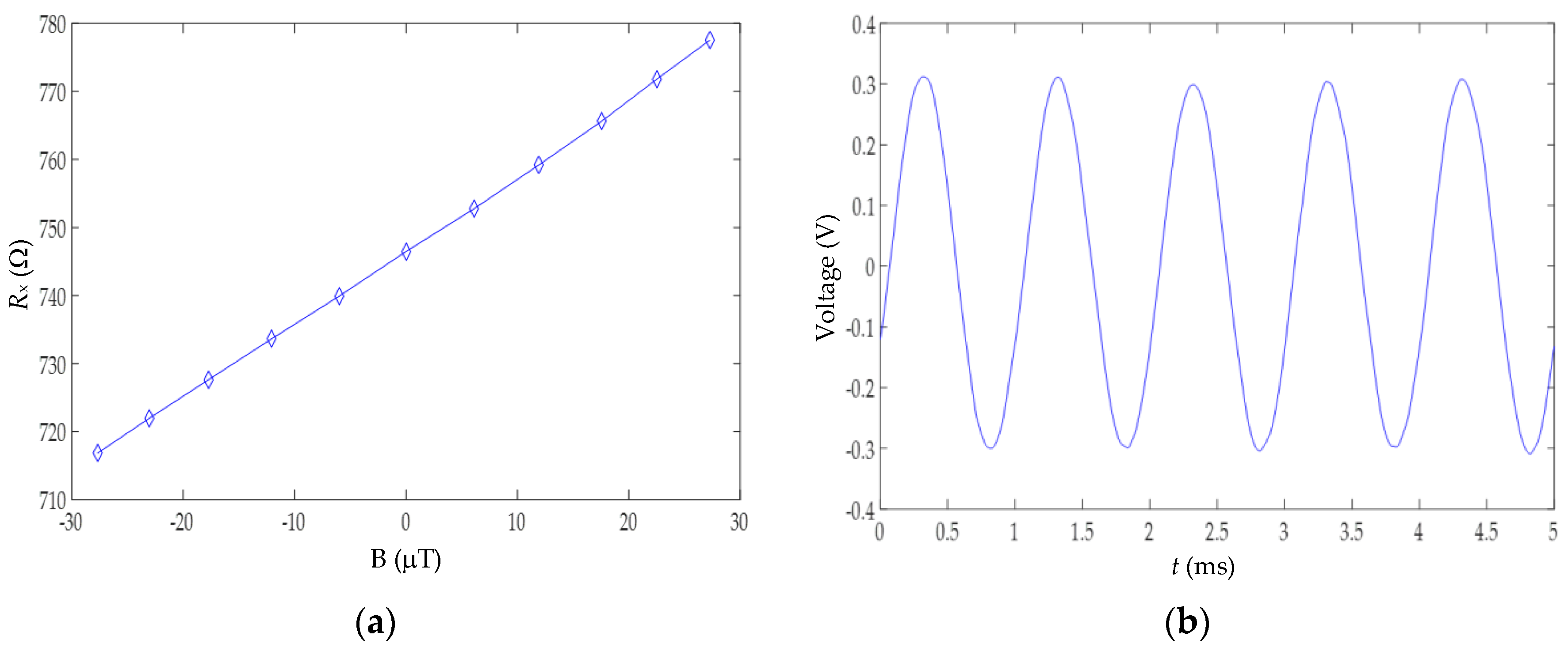
4. Materials and Method
- (a)
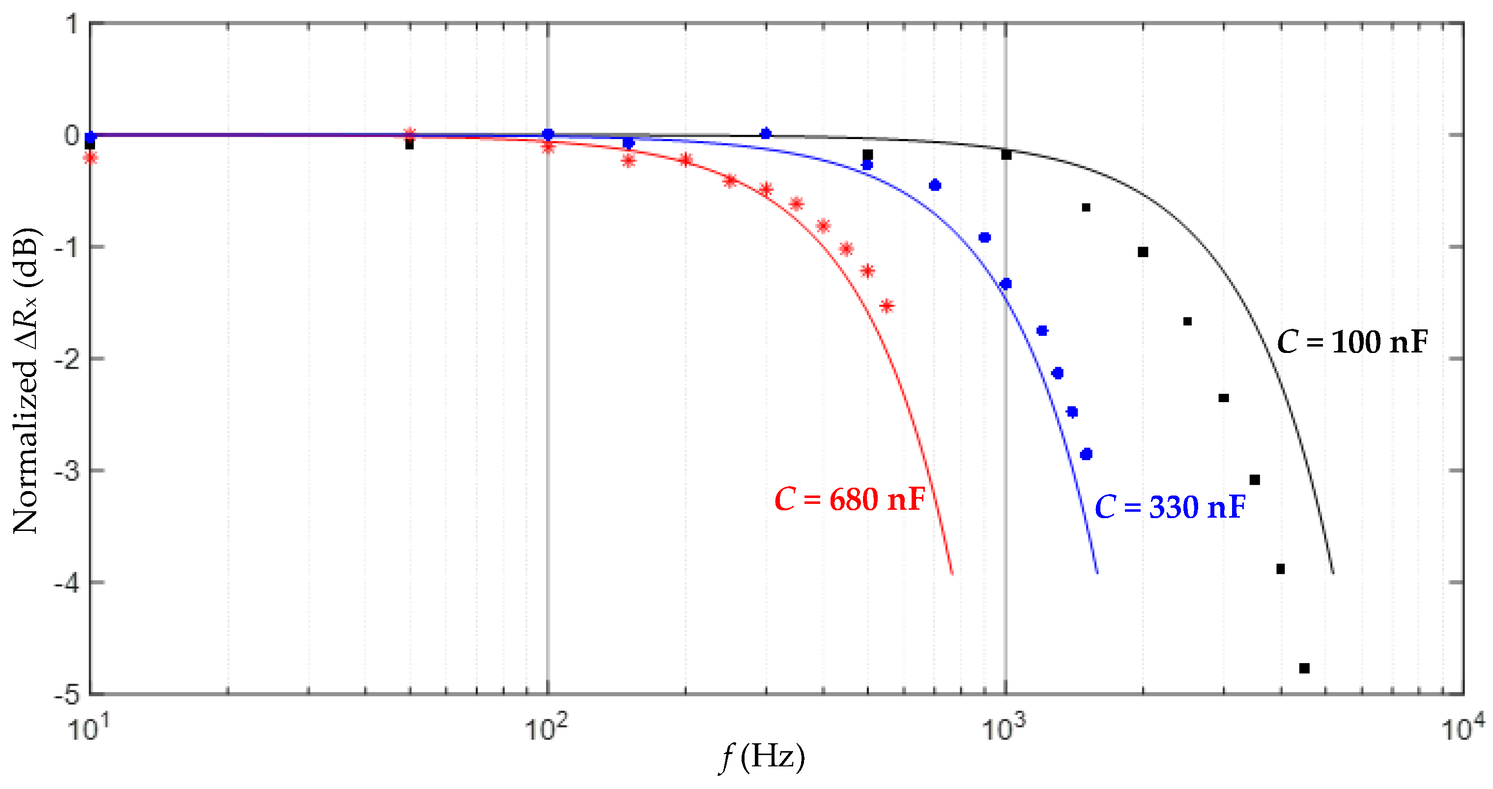
- Experiment A, which was intended to observe the effects of frequency. The frequency of B(t) was varied from 10 Hz to the Nyquist frequency, the amplitude was the maximum (corresponding to a peak-to-peak amplitude of 20 V from the generator), and the waveform was sinusoidal. Three different values of C were tested: 100 nF, 330 nF, and 680 nF.
- (b)
- Experiment B, which was intended to observe the effects of amplitude. The frequency of B(t) was constant, the amplitude had three different levels (corresponding to a peak-to-peak amplitude of 5, 10, and 20 V from the generator), and the waveform was sinusoidal. A frequency of 1 kHz and a capacitor of 100 nF were selected. As shown later after presenting the results of Experiment A, this is the highest frequency that can be tested without the effects of the inherent LPF; note, from Table 1, that fs ≈ 10f when C = 100 nF and, hence, the attenuation factor is 0.1 dB. A higher frequency value could be tested using a smaller value of C, but then the resolution would be smaller than eight bits, which is usually considered as the minimum value in electronic instrumentation.
- (c)
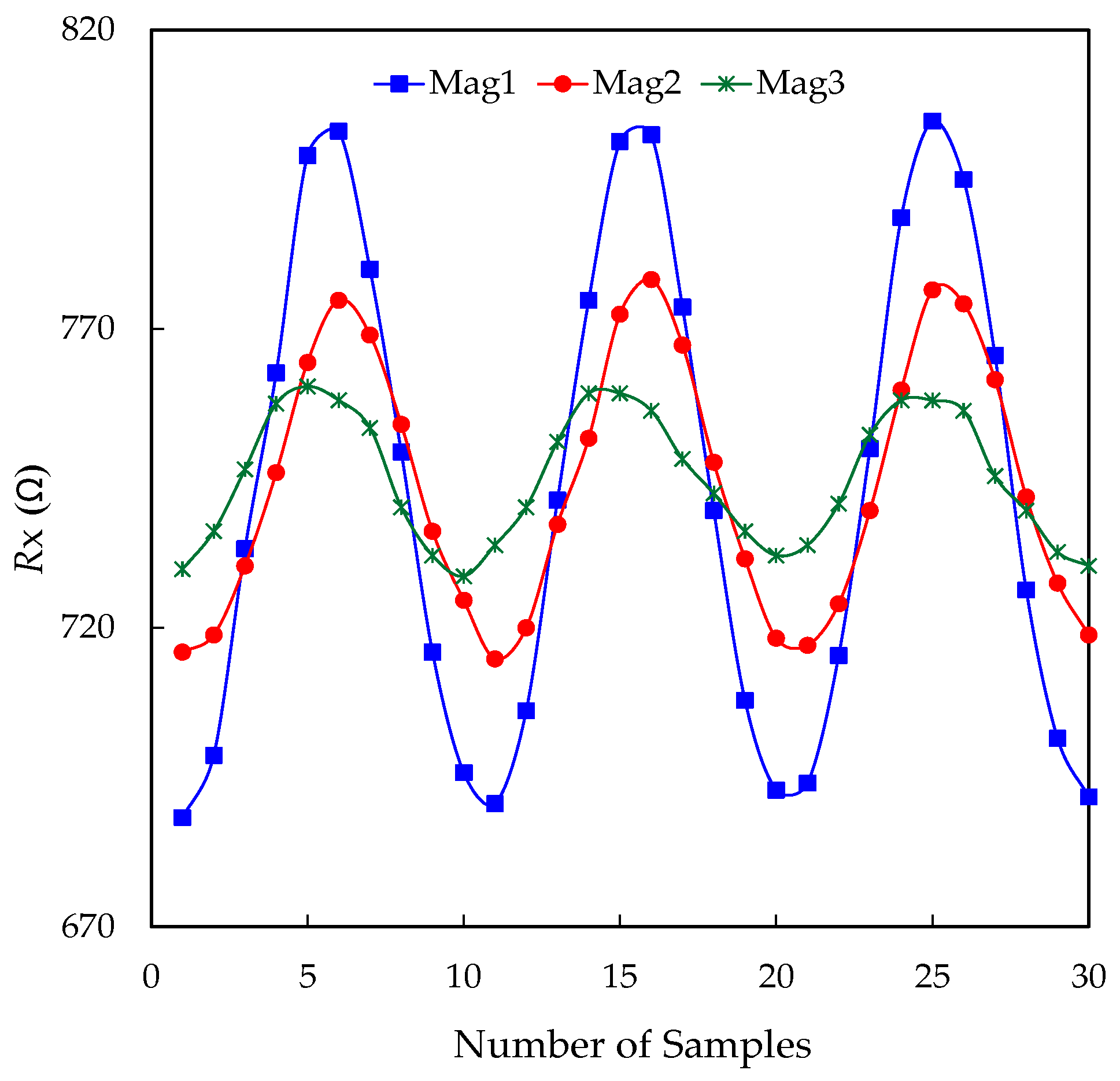
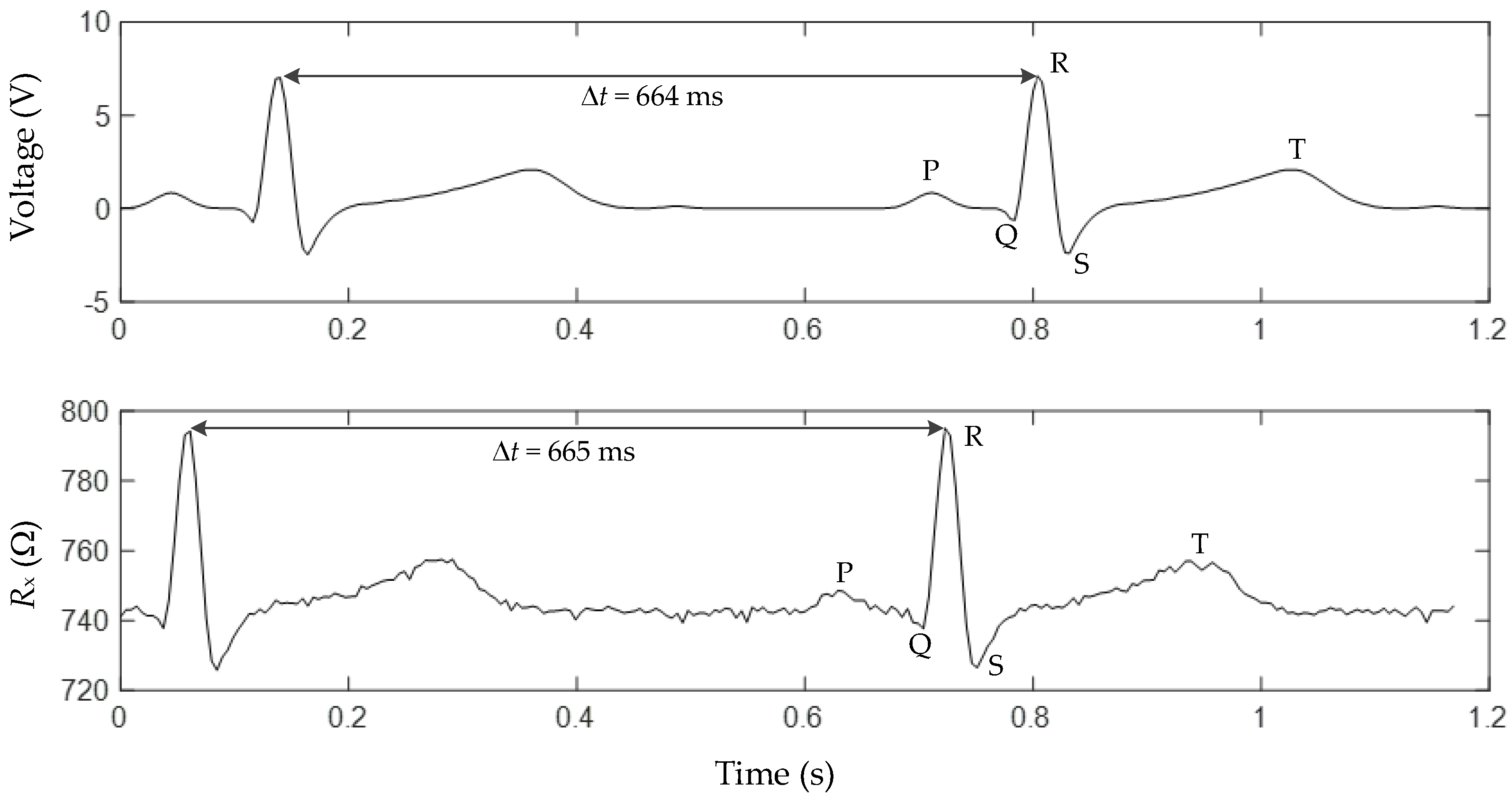
- Experiment C, which was intended to observe the effects of the waveform. The inductor was excited with a narrowband signal with different amplitudes and frequency components. To be precise, the excitation signal emulated an electrocardiogram (ECG) signal with a fundamental frequency of 1.5 Hz that corresponds to a heart rate of 90 beats per minute. ECG monitoring requires a read-out circuit whose bandwidth should be no less than 40 Hz [24]. In order to have such a bandwidth and also optimize the performance of the DIC in terms of resolution, a capacitor of 4.7 μF was selected. This capacitor provides, from Equation (3), a sampling frequency of around 200 Sa/s and, from Equation (8), a 3-dB cut-off frequency of 90 Hz. The ECG signal applied to the inductor was also monitored by the digital oscilloscope.
5. Experimental Results and Discussion
6. Conclusions
Acknowledgments
Author Contributions
Conflicts of Interest
References
- Reverter, F.; Jordana, J.; Gasulla, M.; Pallàs-Areny, R. Accuracy and resolution of direct resistive sensor-to-microcontroller interfaces. Sens. Actuators A Phys. 2005, 121, 78–87. [Google Scholar] [CrossRef]
- Reverter, F.; Casas, O. Interfacing differential resistive sensors to microcontrollers: A direct approach. IEEE Trans. Instrum. Meas. 2009, 58, 3405–3410. [Google Scholar] [CrossRef]
- Sifuentes, E.; Casas, O.; Reverter, F.; Pallas-Areny, R. Direct interface circuit to linearise resistive sensor bridges. Sens. Actuators A Phys. 2008, 147, 210–215. [Google Scholar] [CrossRef]
- Ponnalagu, R.N.; George, B.; Kumar, V.J. A microcontroller sensor interface suitable for resistive sensors with large lead resistance. In Proceedings of the 8th International Conference Sensing Technology, Liverpool, UK, 2–4 September 2014; pp. 327–331. [Google Scholar]
- Reverter, F.; Casas, O. Direct interface circuit for capacitive humidity sensors. Sens. Actuators A Phys. 2008, 143, 315–322. [Google Scholar] [CrossRef]
- Reverter, F.; Casas, O. Interfacing differential capacitive sensors to microcontrollers: A direct approach. IEEE Trans. Instrum. Meas. 2010, 59, 2763–2769. [Google Scholar] [CrossRef]
- Pelegrí-Sebastiá, J.; García-Breijo, E.; Ibáñez, J.; Sogorb, T.; Laguarda-Miro, N.; Garrigues, J. Low-cost capacitive humidity sensor for application within flexible RFID labels based on microcontroller systems. IEEE Trans. Instrum. Meas. 2012, 61, 545–553. [Google Scholar] [CrossRef]
- Chetpattananondh, K.; Tapoanoi, T.; Phukpattaranont, P.; Jindapetch, N. A self-calibration water level measurement using an interdigital capacitive sensor. Sens. Actuators A Phys. 2014, 209, 175–182. [Google Scholar] [CrossRef]
- Kokolanski, Z.; Jordana, J.; Gasulla, M.; Dimcev, V.; Reverter, F. Direct inductive sensor-to-microcontroller interface circuit. Sens. Actuators A Phys. 2015, 224, 185–191. [Google Scholar] [CrossRef]
- Ramadoss, N.; George, B. A simple microcontroller based digitizer for differential inductive sensors. In Proceedings of the IEEE International Instrumentation Measurement Technology Conference, Pisa, Italy, 11–14 May 2015. [Google Scholar]
- Bengtsson, L. Direct analog-to-microcontroller interfacing. Sens. Actuators A Phys. 2012, 179, 105–113. [Google Scholar] [CrossRef]
- Dutta, L.; Hazarika, A.; Bhuyan, M. Microcontroller based e-nose for gas classification without using ADC. Sens. Transducers 2016, 202, 38–45. [Google Scholar]
- Reverter, F. The art of directly interfacing sensors to microcontrollers. J. Low Power Electron. Appl. 2012, 2, 265–281. [Google Scholar] [CrossRef]
- Oballe-Peinado, O.; Vidal-Verdú, F.; Sánchez-Durán, J.A.; Castellanos-Ramos, J.; Hidalgo-López, J.A. Accuracy and resolution analysis of a direct resistive sensor array to FPGA interface. Sensors 2016, 16, 181. [Google Scholar] [CrossRef] [PubMed]
- Oballe-Peinado, O.; Vidal-Verdú, F.; Sánchez-Durán, J.A.; Castellanos-Ramos, J.; Hidalgo-López, J.A. Smart capture modules for direct sensor-to-FPGA interfaces. Sensors 2015, 15, 31762–31780. [Google Scholar] [CrossRef] [PubMed]
- Reverter, F. Power consumption in direct interface circuits. IEEE Trans. Instrum. Meas. 2013, 62, 503–509. [Google Scholar] [CrossRef]
- Henzler, S. Time-to-Digital Converters; Springer: Dordrecht, The Netherlands, 2010; ISBN 978-90-481-8627-3. [Google Scholar]
- Bengtsson, L. Embedded Measurement Systems. Ph.D. Thesis, Department of Physics, University of Gothenburg, Gothenburg, Sweden, 2013. [Google Scholar]
- Sifuentes, E.; Cota-Ruiz, J.; González-Landaeta, R. Respiratory rate detection by a time-based measurement system. Rev. Mex. Ing. Bioméd. 2016, 37, 1–9. [Google Scholar] [CrossRef]
- Hoeschele, D.F. Analog-To-Digital and Digital-To-Analog Conversion Techniques; John Wiley & Sons: New York, NY, USA, 1994; ISBN 978-0-471-57147-6. [Google Scholar]
- Westra, J.R.; Verhoeven, C.J.M.; van Roermund, A.H.M. Oscillators and Oscillator Systems. Classification, Analysis and Synthesis; Kluwer Academic Publishers: Boston, MA, USA, 1999; ISBN 978-0-7923-8652-0. [Google Scholar]
- Reverter, F.; Gasulla, M.; Pallàs-Areny, R. Analysis of power supply interference effects on quasi-digital sensors. Sens. Actuators A Phys. 2005, 119, 187–195. [Google Scholar] [CrossRef]
- Reverter, F.; Pallàs-Areny, R. Effective number of resolution bits in direct sensor-to-microcontroller interfaces. Meas. Sci. Technol. 2004, 15, 2157–2162. [Google Scholar] [CrossRef]
- ANSI/AAMI EC13: 2002/(R2007). Cardiac Monitors, Heart Rate Meters, and Alarms; ANSI Standard: Arlington, VA, USA, 2002. [Google Scholar]
- Webster, J. Medical Instrumentation: Application and Design; John Wiley & Sons: New York, NY, USA, 2009; ISBN 978-0-471-67600-3. [Google Scholar]


| C (nF) | fs (kSa/s) 1 | n (bits) 2 | Δr (mΩ) 3 |
|---|---|---|---|
| 100 | 10.47 | 7.7 | 577 |
| 330 | 3.17 | 9.4 | 175 |
| 680 | 1.54 | 10.5 | 83 |
© 2017 by the authors. Licensee MDPI, Basel, Switzerland. This article is an open access article distributed under the terms and conditions of the Creative Commons Attribution (CC BY) license (http://creativecommons.org/licenses/by/4.0/).
Share and Cite
Sifuentes, E.; Gonzalez-Landaeta, R.; Cota-Ruiz, J.; Reverter, F. Measuring Dynamic Signals with Direct Sensor-to-Microcontroller Interfaces Applied to a Magnetoresistive Sensor. Sensors 2017, 17, 1150. https://doi.org/10.3390/s17051150
Sifuentes E, Gonzalez-Landaeta R, Cota-Ruiz J, Reverter F. Measuring Dynamic Signals with Direct Sensor-to-Microcontroller Interfaces Applied to a Magnetoresistive Sensor. Sensors. 2017; 17(5):1150. https://doi.org/10.3390/s17051150
Chicago/Turabian StyleSifuentes, Ernesto, Rafael Gonzalez-Landaeta, Juan Cota-Ruiz, and Ferran Reverter. 2017. "Measuring Dynamic Signals with Direct Sensor-to-Microcontroller Interfaces Applied to a Magnetoresistive Sensor" Sensors 17, no. 5: 1150. https://doi.org/10.3390/s17051150
APA StyleSifuentes, E., Gonzalez-Landaeta, R., Cota-Ruiz, J., & Reverter, F. (2017). Measuring Dynamic Signals with Direct Sensor-to-Microcontroller Interfaces Applied to a Magnetoresistive Sensor. Sensors, 17(5), 1150. https://doi.org/10.3390/s17051150