
A Novel Method to Enhance Pipeline Trajectory Determination Using Pipeline Junctions


Abstract
:
1. Introduction
2. New Information
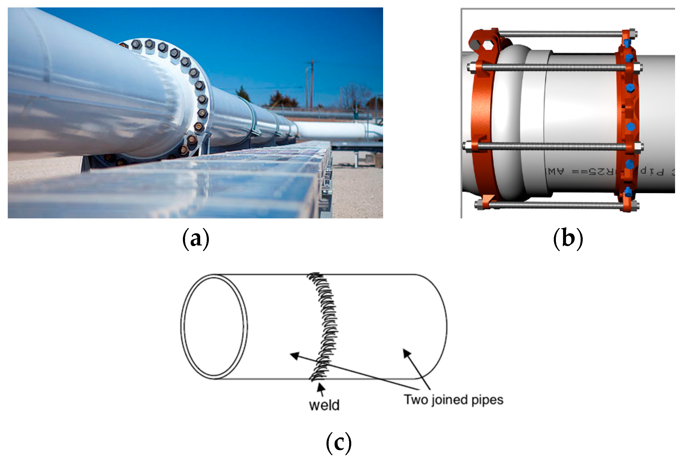
2.1. Pipeline Junctions
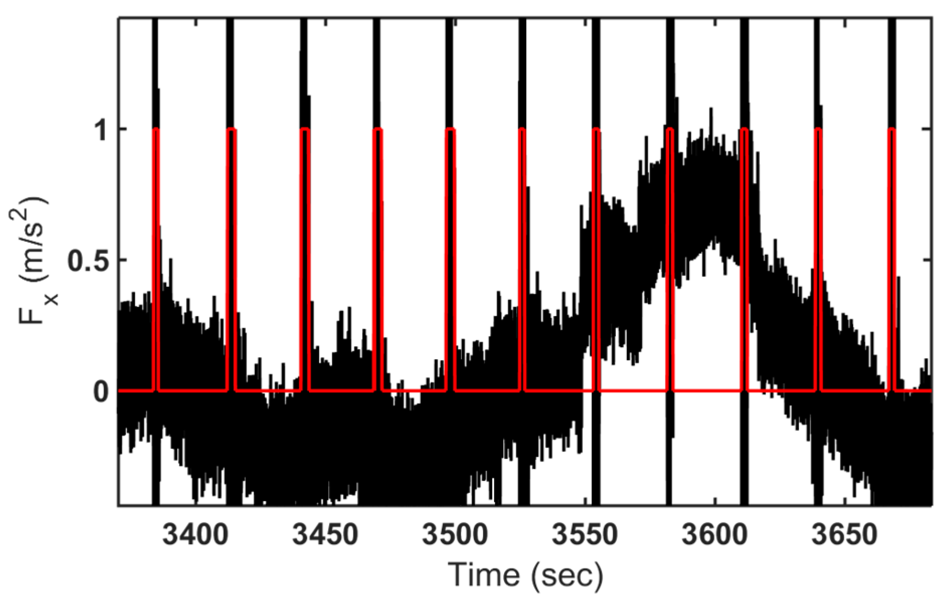
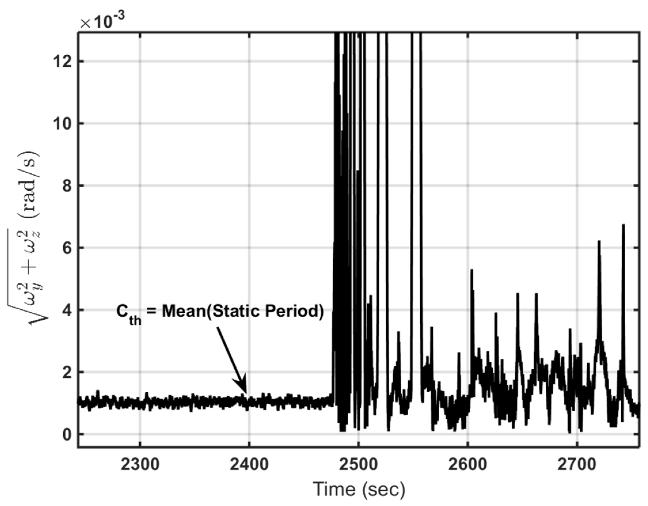
2.2. Detecting Pipeline Junctions
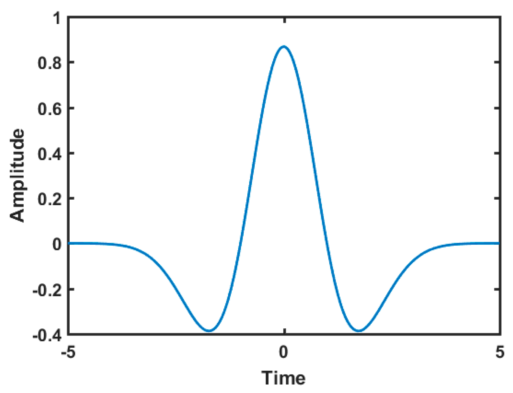
2.3. Bend Detection Algorithm (BDA)
3. Methodology
3.1. Dynamic Error Model
- Position error
- Velocity error
- Attitude error
- Gyroscope bias error
- Accelerometer bias error .
- :
- is the state vector
- :
- is the transition matrix
- :
- is the noise distribution matrix
- :
- is the unit-variance white Gaussian noise.
- Reciprocal of the correlation time of the process
- Variance of the white noise associated with the random process
- Meridian radius of curvature (North-South)
- Prime vertical radius of curvature of the Earth’s surface (East-West)
- Latitude, longitude and height, respectively
- Specific forces in east, north and up directions, respectively.
- Rotation matrix elements from body to local level frame.
- Rate change of time.
3.2. Pitch & Heading Measurement Model
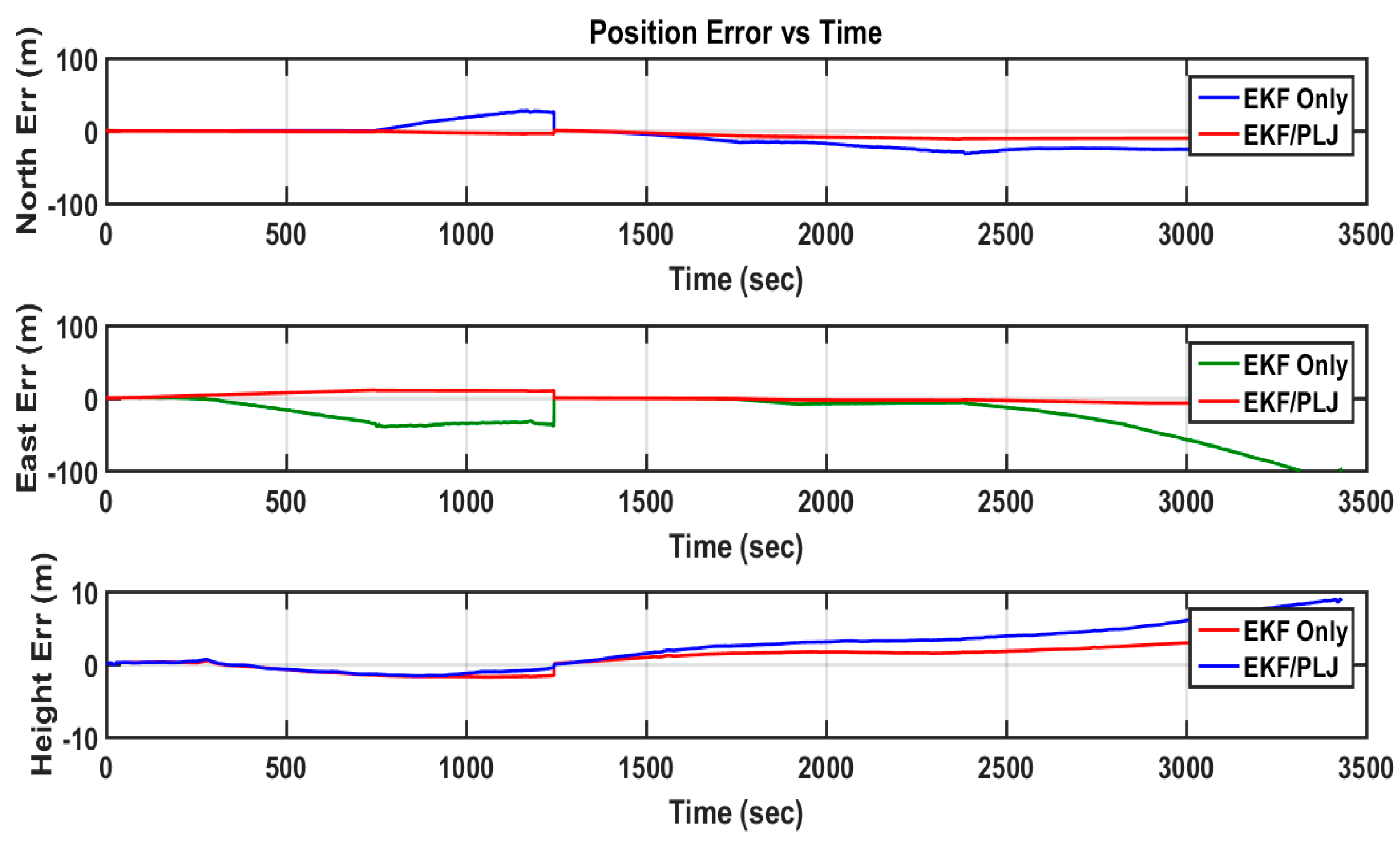
4. Results
- •
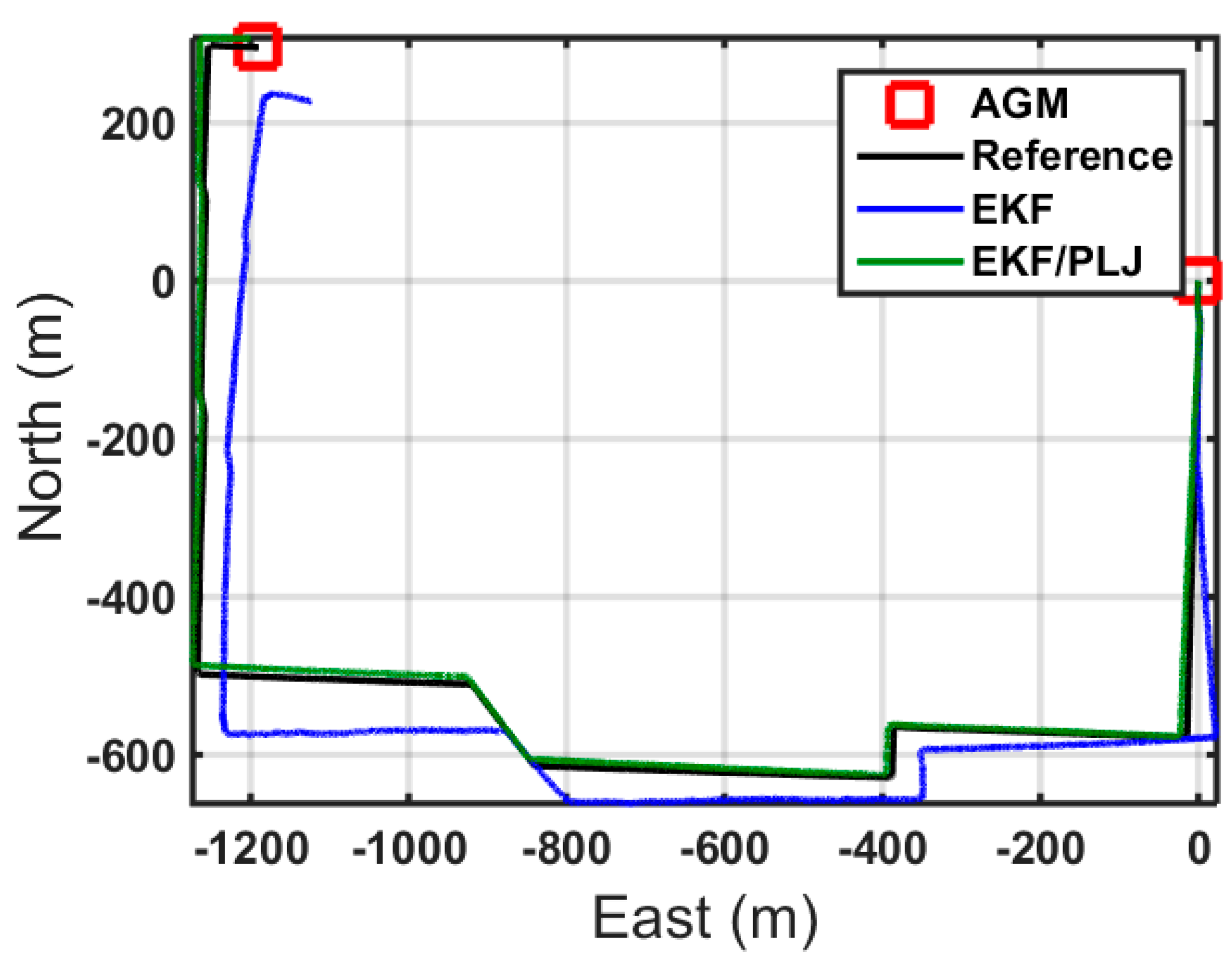
- Scenario #1: Processed IMU & odometer data using one AGM (after )
- •
- Scenario #2: Processed IMU & odometer data using no AGM.
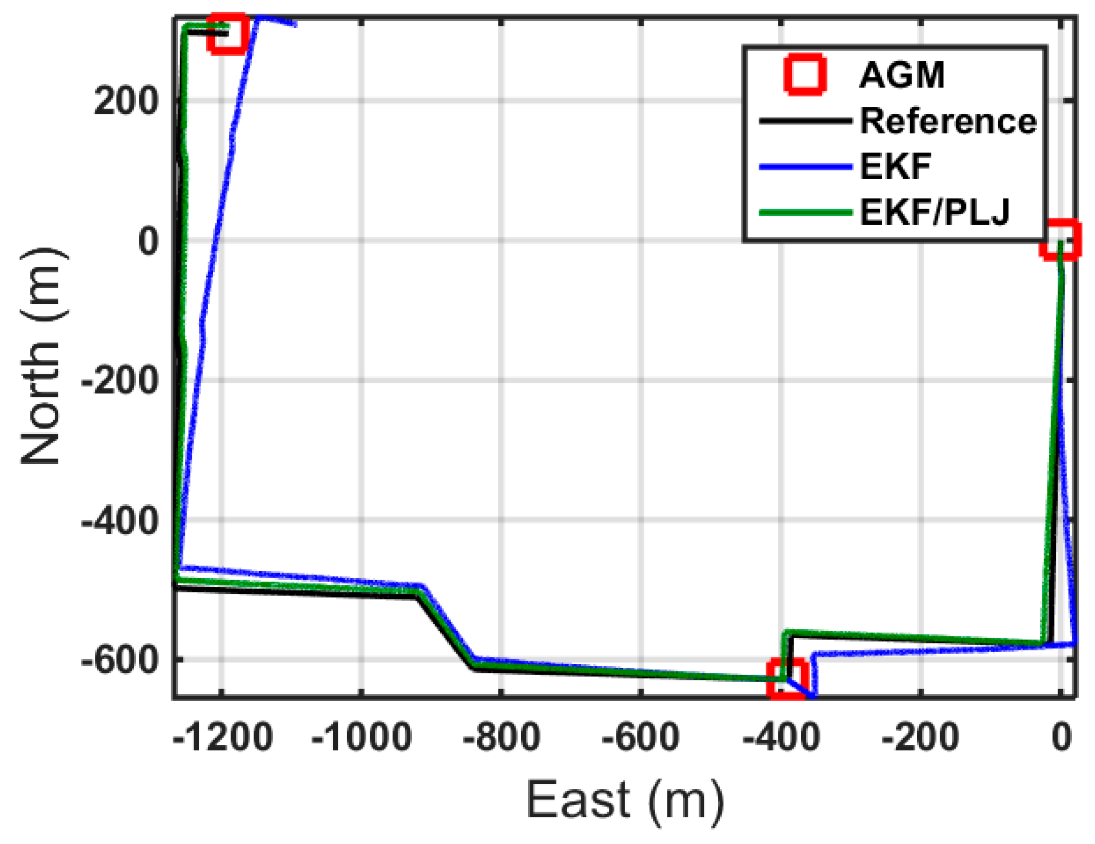
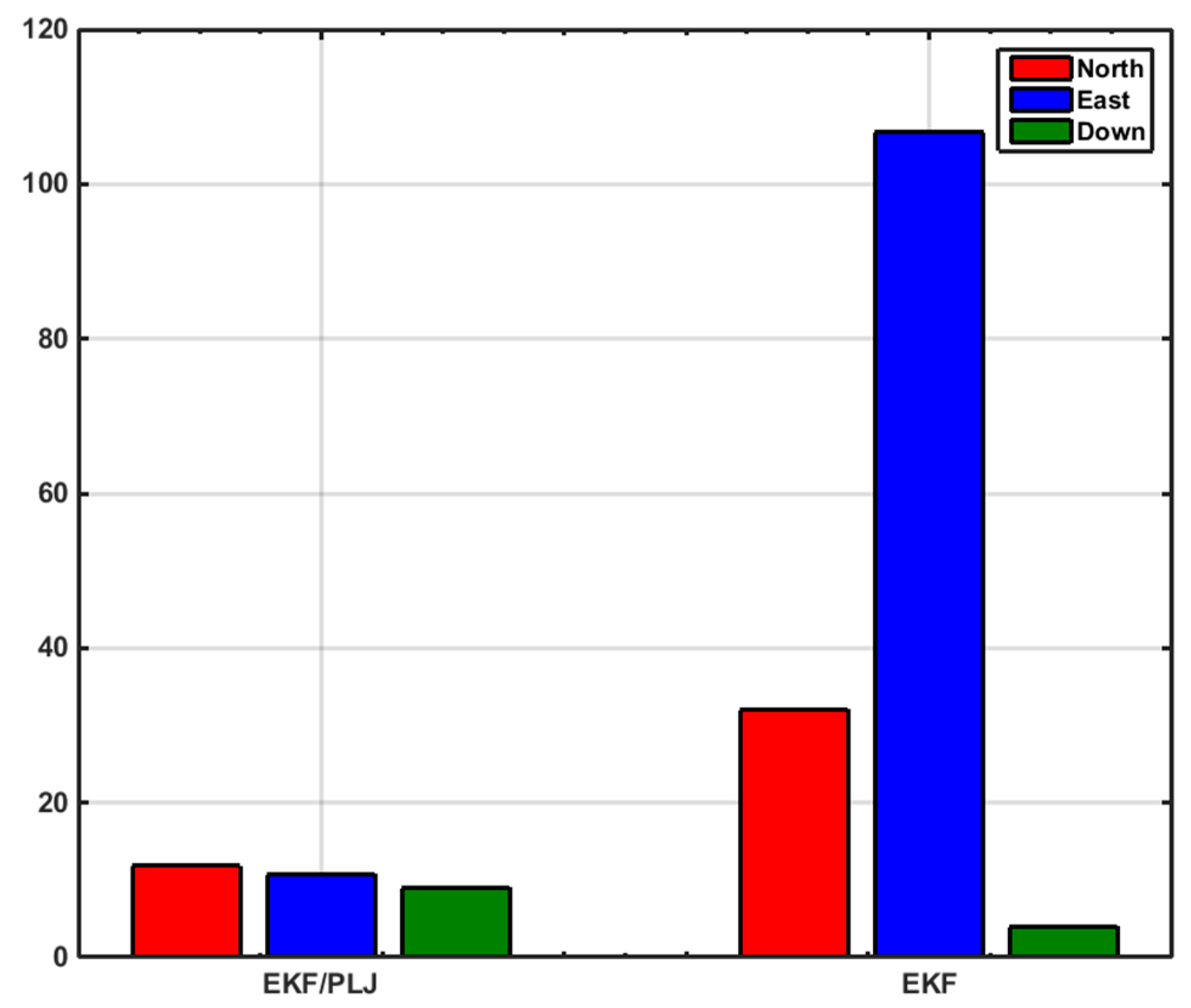
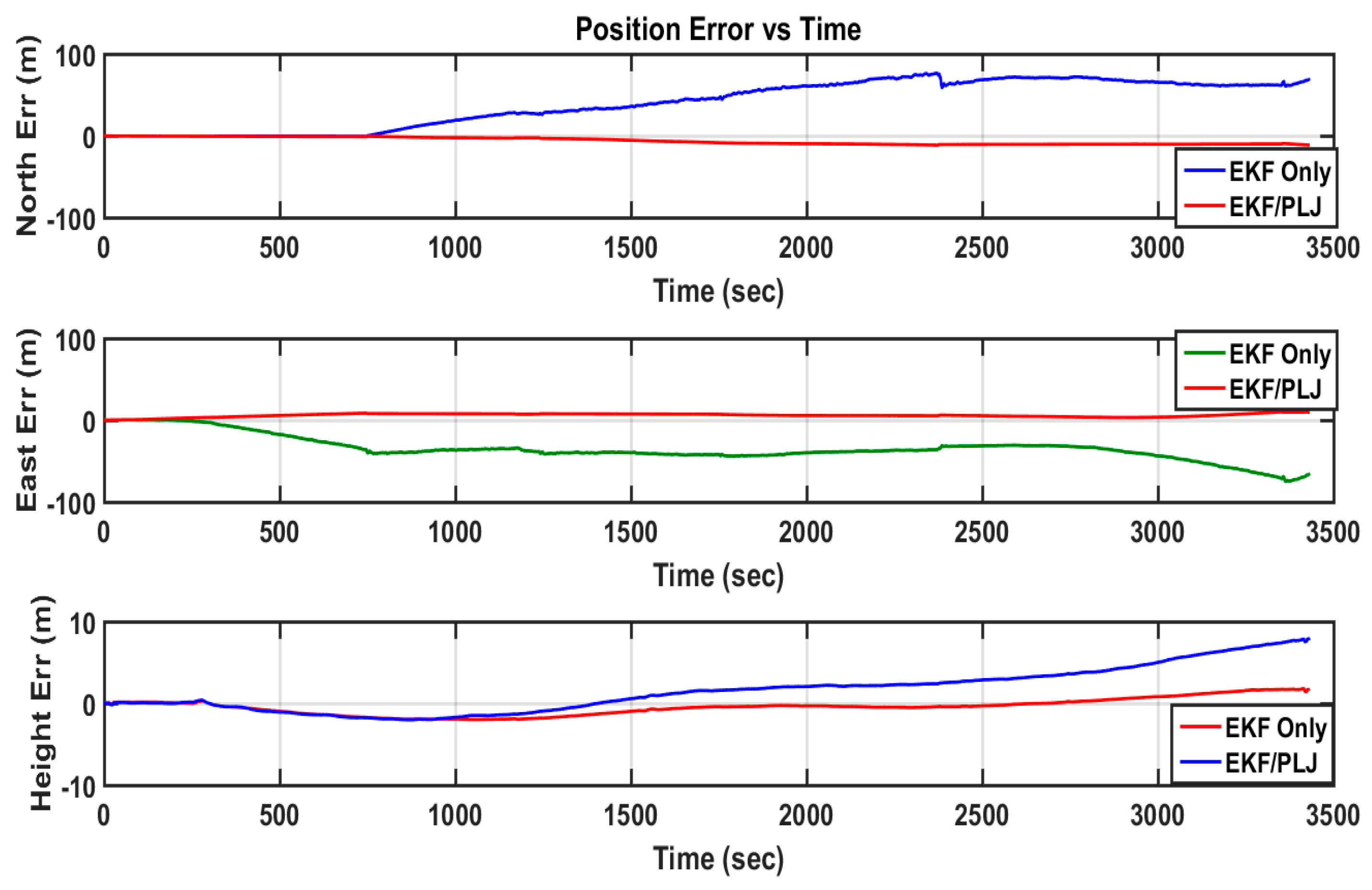
4.1. Scenario #1
4.2. Scenario #2
5. Conclusions
Acknowledgments
Author Contributions
Conflicts of Interest
Appendix A
References
- Tiratsoo, J. Pipeline Pigging Technology, 2nd ed.; Butterworth-Heinemann College: Woburn, MA, USA, 2001. [Google Scholar]
- Tolmasquim, S.T.; Nieckele, A.O. Design and control of pig operations through pipelines. J. Pet. Sci. Eng. 2008, 62, 102–110. [Google Scholar] [CrossRef]
- Davidson, R. An Introduction to Pipeline Pigging: Pigging Products & Services Association; Pipes & Pipelines International: Beaconsfield, UK, 1995. [Google Scholar]
- Hanna, P.L. Strapdown inertial systems for pipeline navigation. In Proceedings of the IEE Colloquium on Inertial Navigation Sensor Development, London, UK, 9 January 1990.
- Sahli, H.; Moussa, A.; Noureldin, A.; El-Sheimy, N. Small pipeline trajectory estimation using MEMS based IMU. In Proceedings of the 27th International Technical Meeting of the Satellite Division of the Institute of Navigation (ION GNSS+ 2014), Tampa, FL, USA, 8–12 September 2014.
- Santana, D.D.S.; Maruyama, N.; Massatoshi Furukawa, C. Estimation of trajectories of pipeline PIGs using inertial measurements and non linear sensor fusion. In Proceedings of the 2010 9th IEEE/IAS International Conference on Industry Applications (INDUSCON), Sao Paulo, Brazil, 8–10 November 2010.
- Chowdhury, M.S.; Abdel-Hafez, M.F. Pipeline Inspection Gauge Position Estimation Using Inertial Measurement Unit, Odometer, and a Set of Reference Stations. ASME. ASME J. Risk Uncertain. Part B 2016, 2, 021001-1–021001-10. [Google Scholar] [CrossRef]
- Grewal, M.S.; Andrews, A.P. Kalman Filtering: Theory and Practice Using MATLAB; John Wiley & Sons, Inc.: Hoboken, NJ, USA, 2015. [Google Scholar]
- Kalman, R.E. A new approach to linear filtering and prediction problems. J. Basic Eng. 1960, 82, 35–45. [Google Scholar] [CrossRef]
- Graps, A. An introduction to wavelets. IEEE Comput. Sci. Eng. 1995, 2, 50–61. [Google Scholar] [CrossRef]
- Mesa, H. Adapted wavelets for pattern detection. In Progress in Pattern Recognition, Image Analysis and Applications; Sanfeliu, A., Cortés, M., Eds.; Springer Berlin Heidelberg: Berlin/Heidelberg, Germany, 2005; pp. 933–944. [Google Scholar]
- Meyer, Y. Wavelets: Algorithms and Applications, 1st ed.; Society for Industrial & Applied: Philadelphia, PA, USA, 1993. [Google Scholar]
- Vetterli, M.; Herley, C. Wavelet and filter banks: Theory and design. IEEE Trans. Acoust. Speech Signal Process. 1992, 40, 2207–2232. [Google Scholar] [CrossRef]
- Wickerhauser, M.V. Adapted Wavelet Analysis from Theory to Software, 1st ed.; A K Peters/CRC Press: Wellesley, MA, USA, 1994. [Google Scholar]
- El-Sheimy, N.; Sahli, H.; Moussa, A. Methods and Systems to Enhance Pipeline Trajectory Reconstruction Using Pipeline Junctions. Patent Tech. ID# 524.28, 7 July 2015. [Google Scholar]
- Noureldin, A.; Karamat, T.B.; Eberts, M.D.; El-Shafie, A. Performance enhancement of mems-based INS/GPS integration for low-cost navigation applications. IEEE Trans. Veh. Technol. 2009, 58, 1077–1096. [Google Scholar] [CrossRef]
- El-Sheimy, N. Introduction to INS—With Applications to Positioning and Mapping; ENGO623 Course Notes; University of Calgary: Calgary, AB, Canada, 2012. [Google Scholar]
- Noureldin, A.; Karamat, T.B.; Georgy, J. Fundamentals of Inertial Navigation, Satellite Positioning and Their Integration; Springer: New York, NY, USA, 2012. [Google Scholar]
- Shin, E.-H. Estimation Techniques for Low-Cost Inertial Navigation; University of Calgary: Calgary, AB, Canada, 2005. [Google Scholar]


| Gyroscope | Accelerometer | |
|---|---|---|
| Bias Repeatability | ≤ 10 mg | |
| Bias Instability | ≤ 0.5 mg | |
| Random Walk | ||
| Size (mm) | Diameter (55.88) | |
| Depth (35.56) | ||
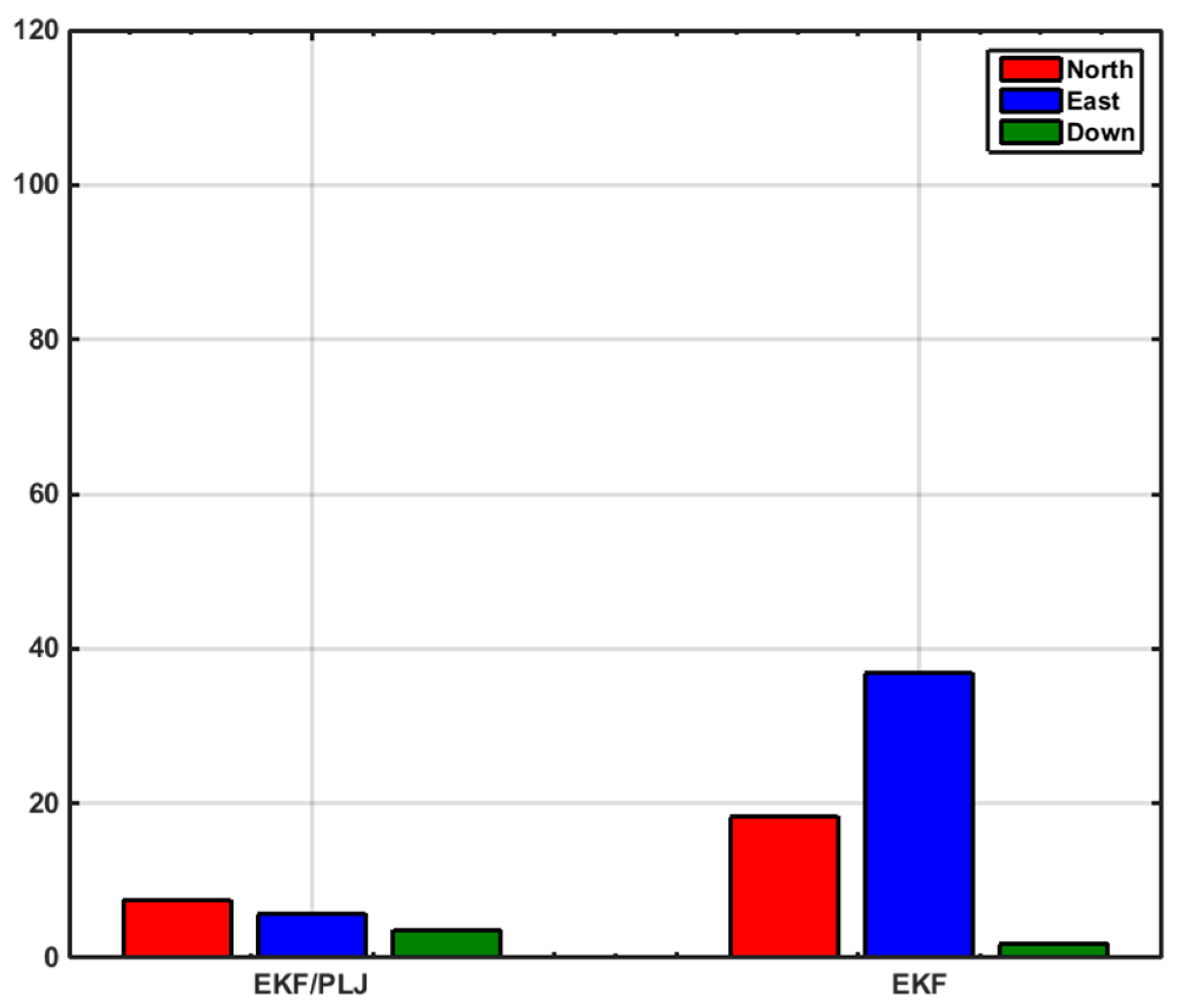
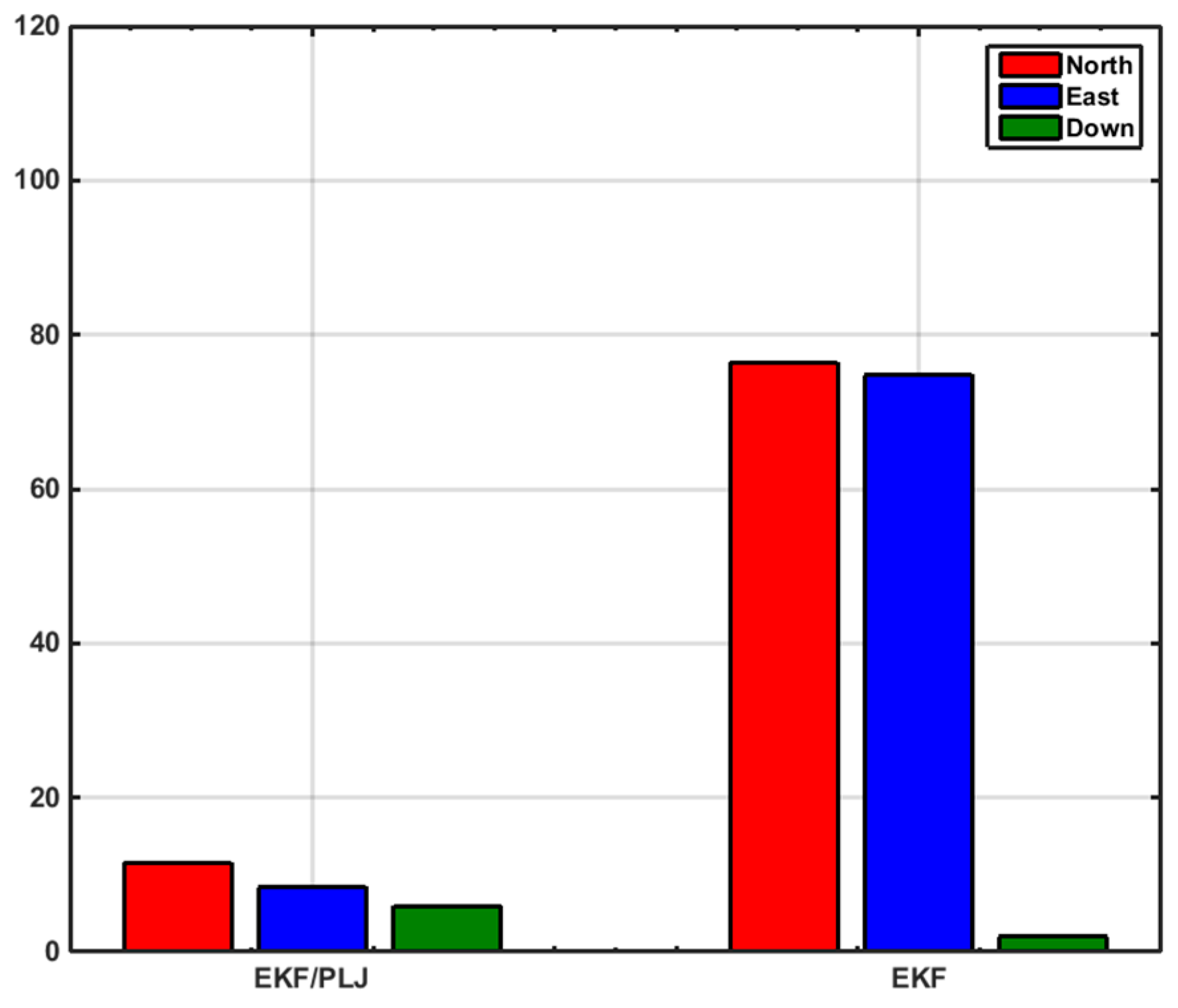
| Maximum Error | ||||
|---|---|---|---|---|
| Method | North (m) | East (m) | Height (m) | |
| Scenario #1 | EKF | 31.99 | 72.89 | 3.28 |
| EKF/PLJ | 11.83 | 10.77 | 7.03 | |
| Scenario #2 | EKF | 76.41 | 51.94 | 1.99 |
| EKF/PLJ | 11.59 | 8.48 | 5.99 | |
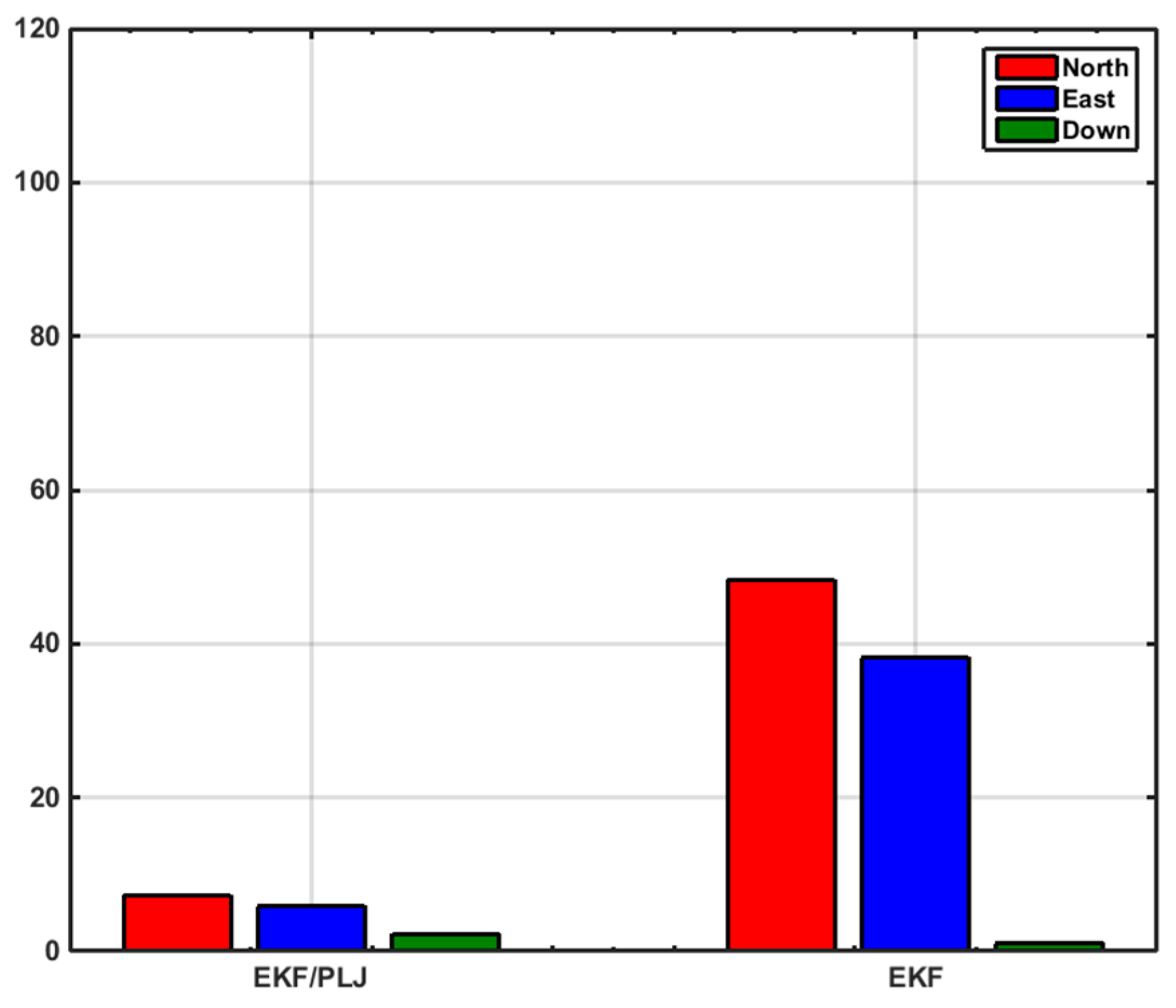
| RMS Error | ||||
|---|---|---|---|---|
| Method | North (m) | East (m) | Height (m) | |
| Scenario #1 | EKF | 17.7 | 25.05 | 1.61 |
| EKF/PLJ | 7.11 | 5.80 | 2.91 | |
| Scenario #2 | EKF | 46.72 | 34.58 | 1.03 |
| EKF/PLJ | 7.35 | 5.91 | 2.31 | |
© 2016 by the authors; licensee MDPI, Basel, Switzerland. This article is an open access article distributed under the terms and conditions of the Creative Commons Attribution (CC-BY) license (http://creativecommons.org/licenses/by/4.0/).
Share and Cite
Sahli, H.; El-Sheimy, N. A Novel Method to Enhance Pipeline Trajectory Determination Using Pipeline Junctions. Sensors 2016, 16, 567. https://doi.org/10.3390/s16040567
Sahli H, El-Sheimy N. A Novel Method to Enhance Pipeline Trajectory Determination Using Pipeline Junctions. Sensors. 2016; 16(4):567. https://doi.org/10.3390/s16040567
Chicago/Turabian StyleSahli, Hussein, and Naser El-Sheimy. 2016. "A Novel Method to Enhance Pipeline Trajectory Determination Using Pipeline Junctions" Sensors 16, no. 4: 567. https://doi.org/10.3390/s16040567
APA StyleSahli, H., & El-Sheimy, N. (2016). A Novel Method to Enhance Pipeline Trajectory Determination Using Pipeline Junctions. Sensors, 16(4), 567. https://doi.org/10.3390/s16040567