
Dynamic Measurement for the Diameter of A Train Wheel Based on Structured-Light Vision


Abstract
:
1. Introduction
2. Measurement Model and Method
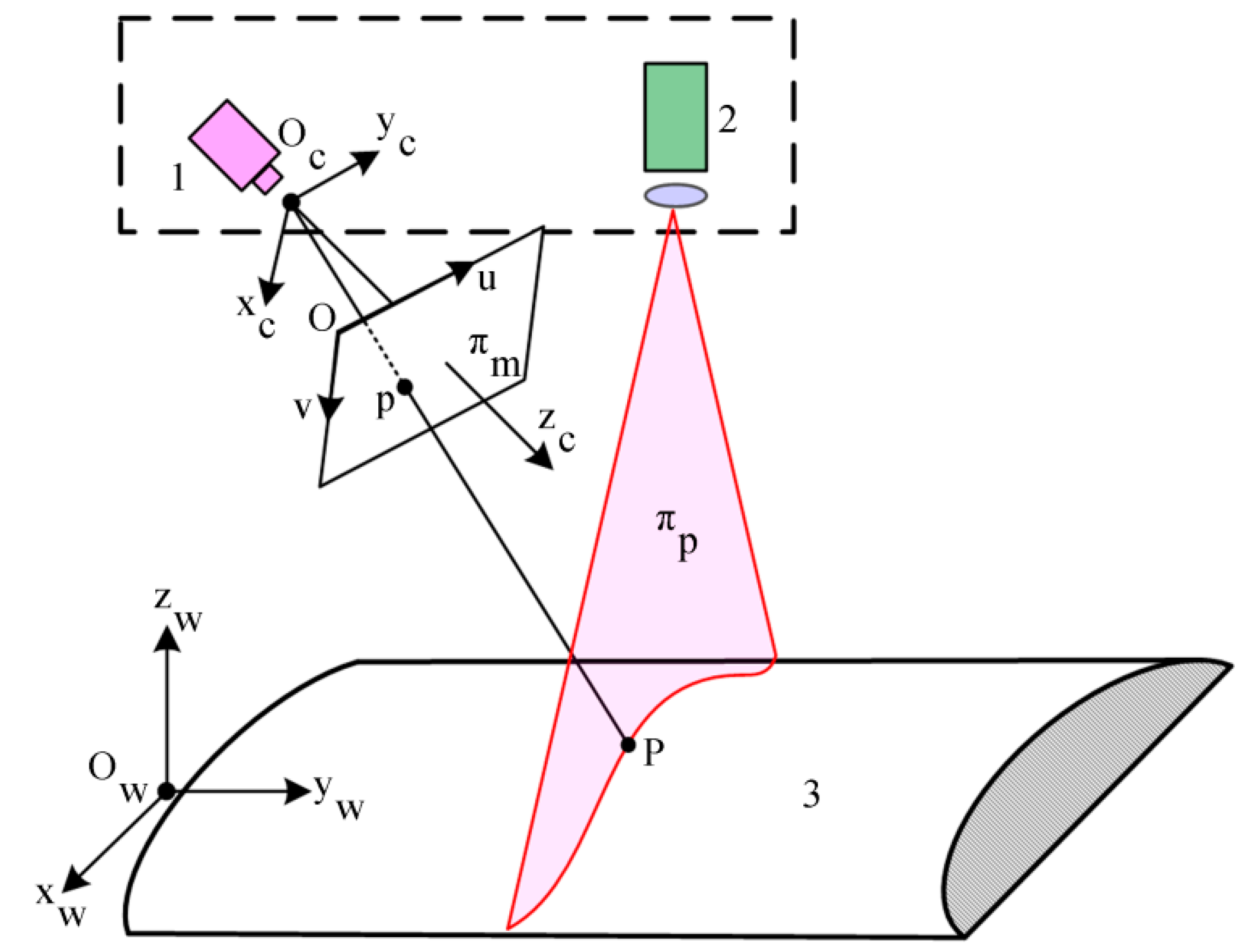
2.1. Structured-Light Vision Model
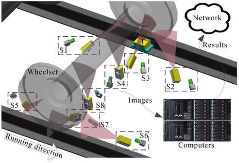
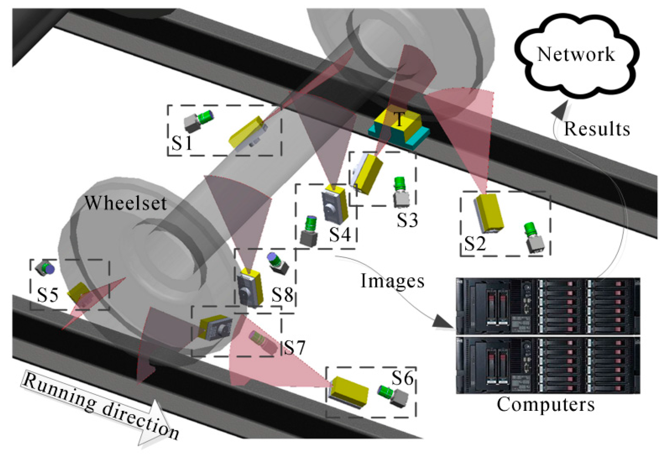
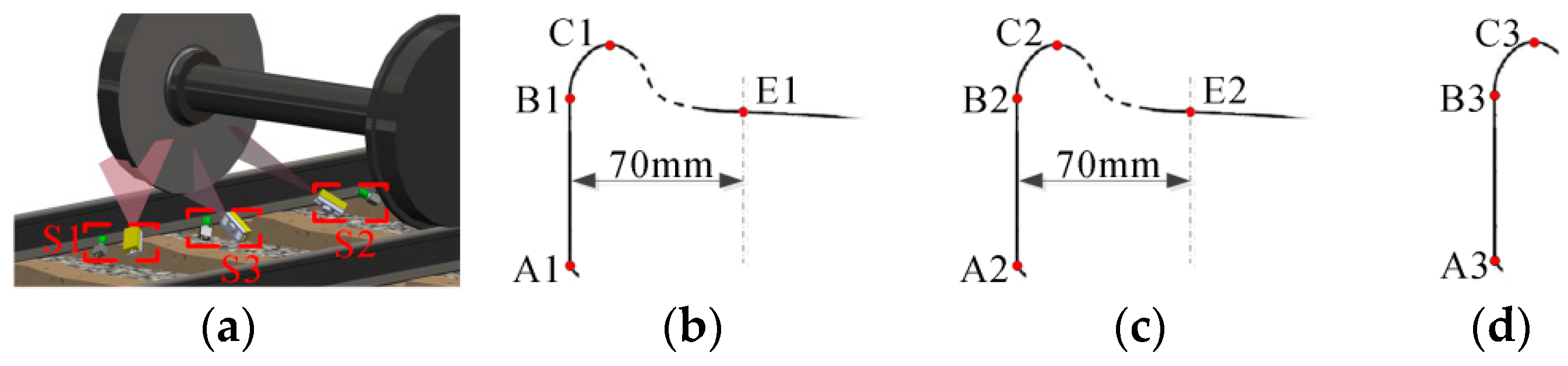
2.2. Configuration of the Structured-Light Sensor
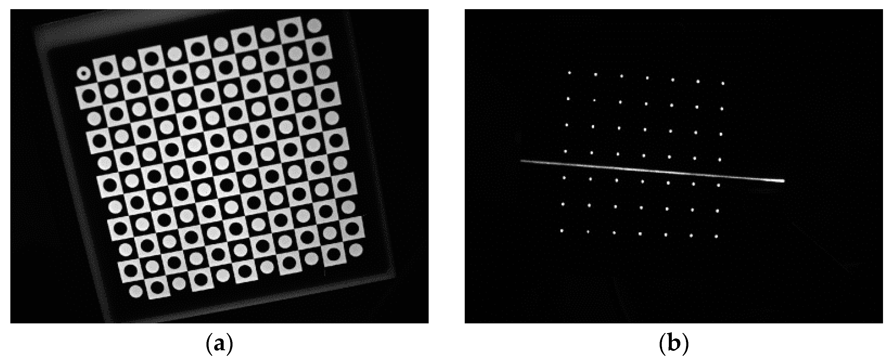
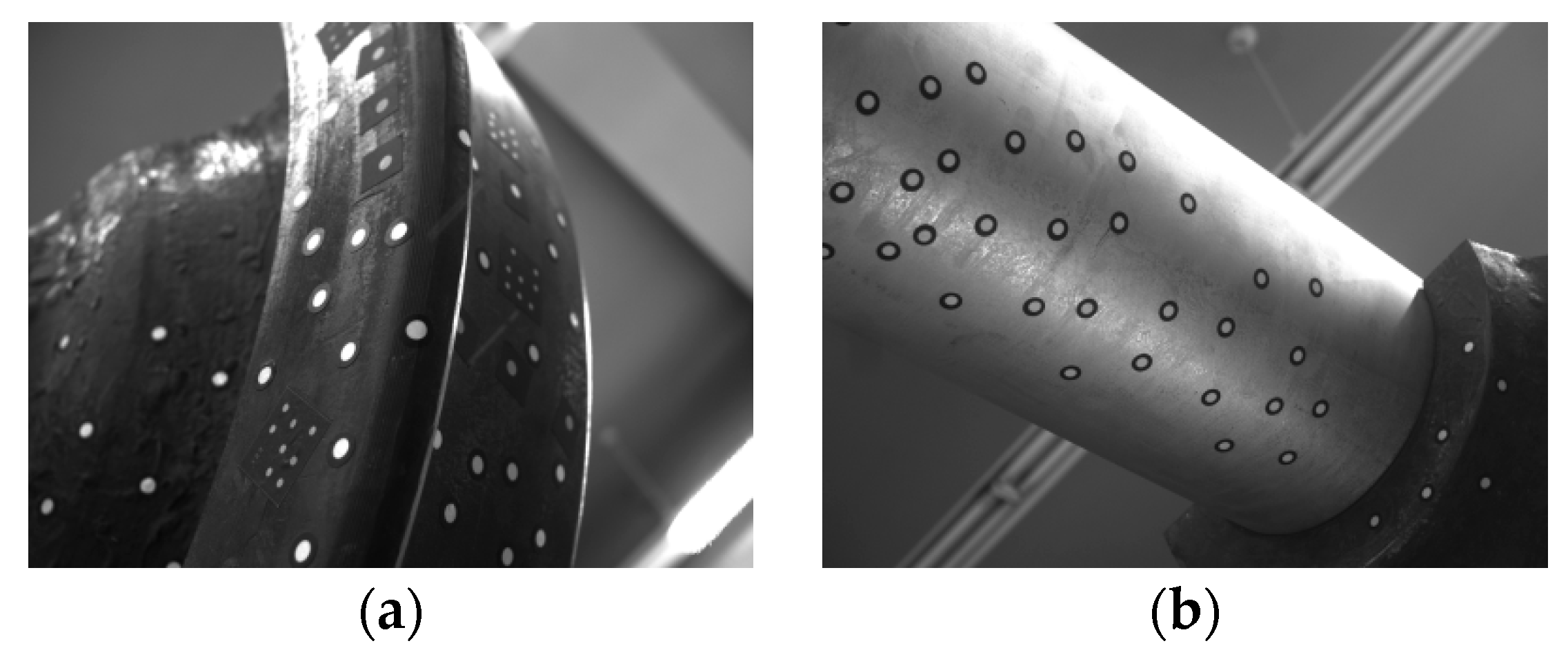
2.3. Calibration of the Structured-Light Vision Model
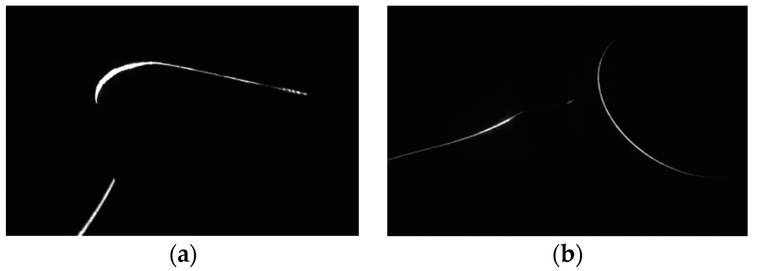
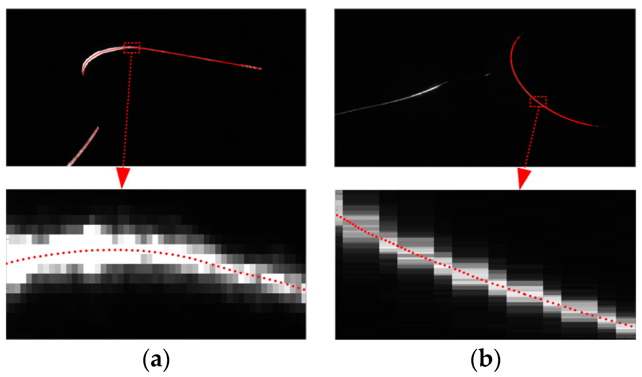
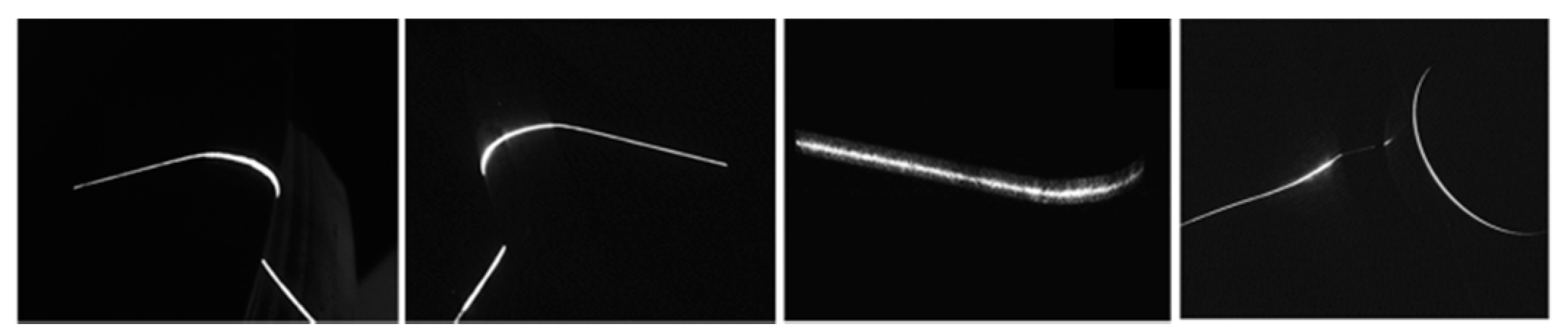
2.4. Image Processing
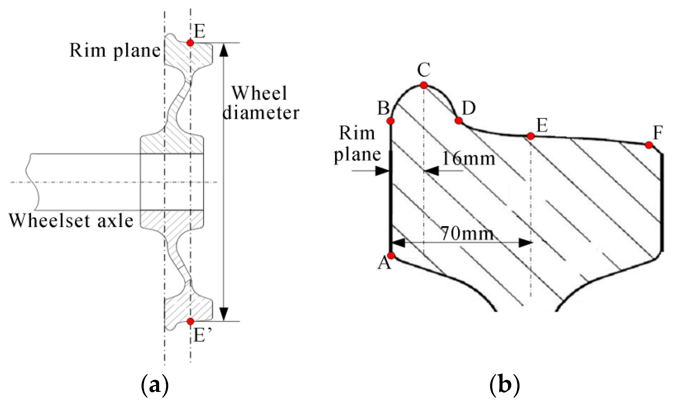
2.5. Wheel Tread Profile and Wheel Diameter
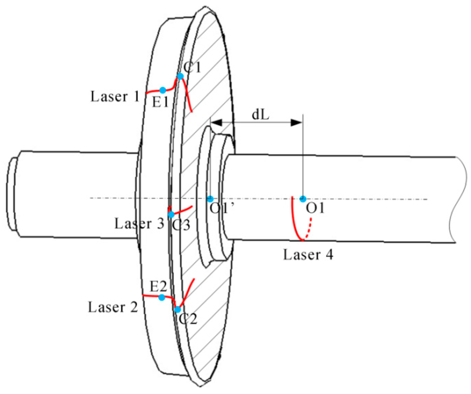
2.6. Calculation of the Diameter
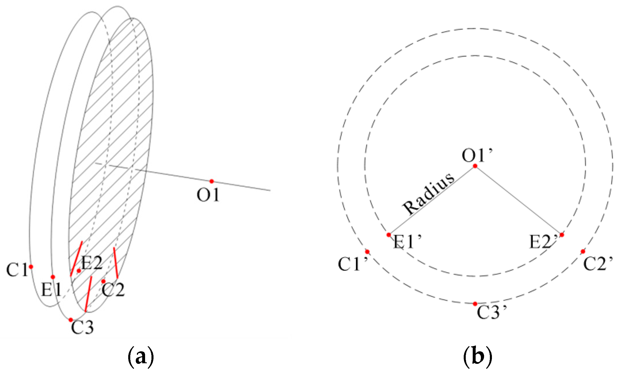
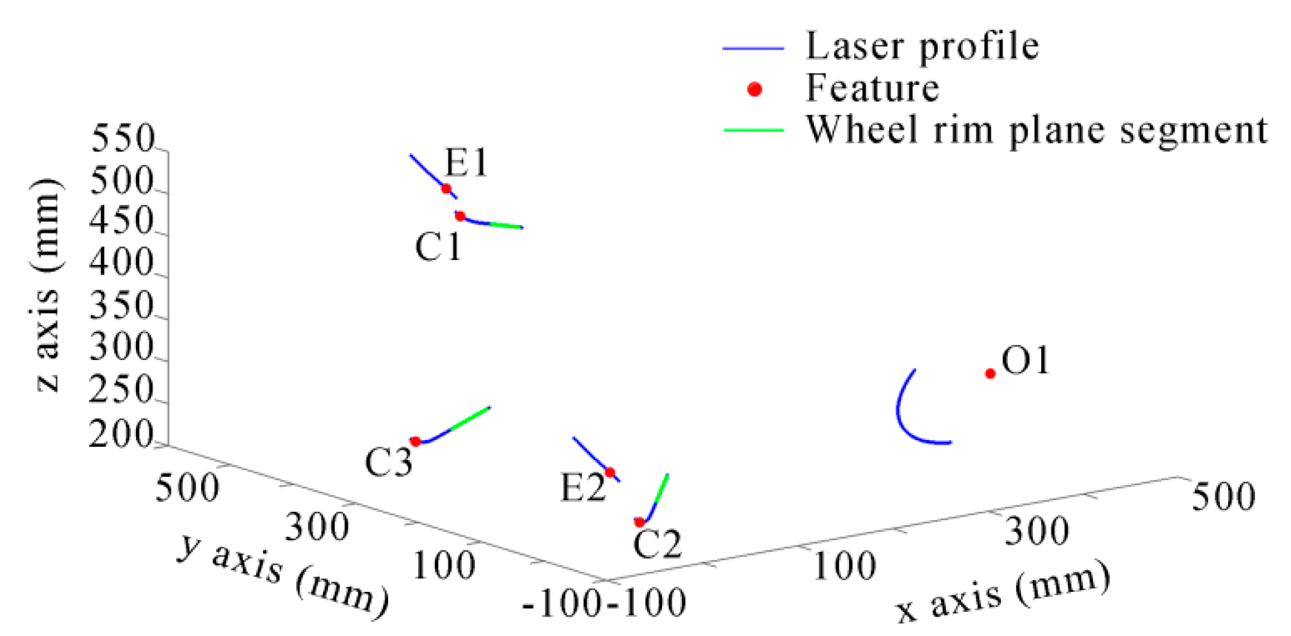
2.6.1. Determine the Rim Plane, the flange Vertex and the Contact Point
- (1)
- Set q0 as the start point of the profile.
- (2)
- In order to avoid the noise and the influence of the wheel spoke, we find the first point q1 satisfying as the start of the straight line.
- (3)
- Generally, the rim plane segment is always longer than 25 mm. We can continue to search the profile, and add all of the points qi satisfying: into the straight line part. Then, the initial straight line can be fitted using these points. The linear least-squares algorithm can be used. Because these points must be a part of the rim plane, the fitting error should be very small.
- (4)
- Add the next point into the straight line part and fit the line again. If the max distance from all of the points to the fitted line is smaller than 0.2 mm, then the point can be added to the straight line part; otherwise, the point should be removed.
- (5)
- Repeat Step (4) with the rest points one by one until the whole profile is searched. Then, we can obtain the rim plane segment and the line equation.
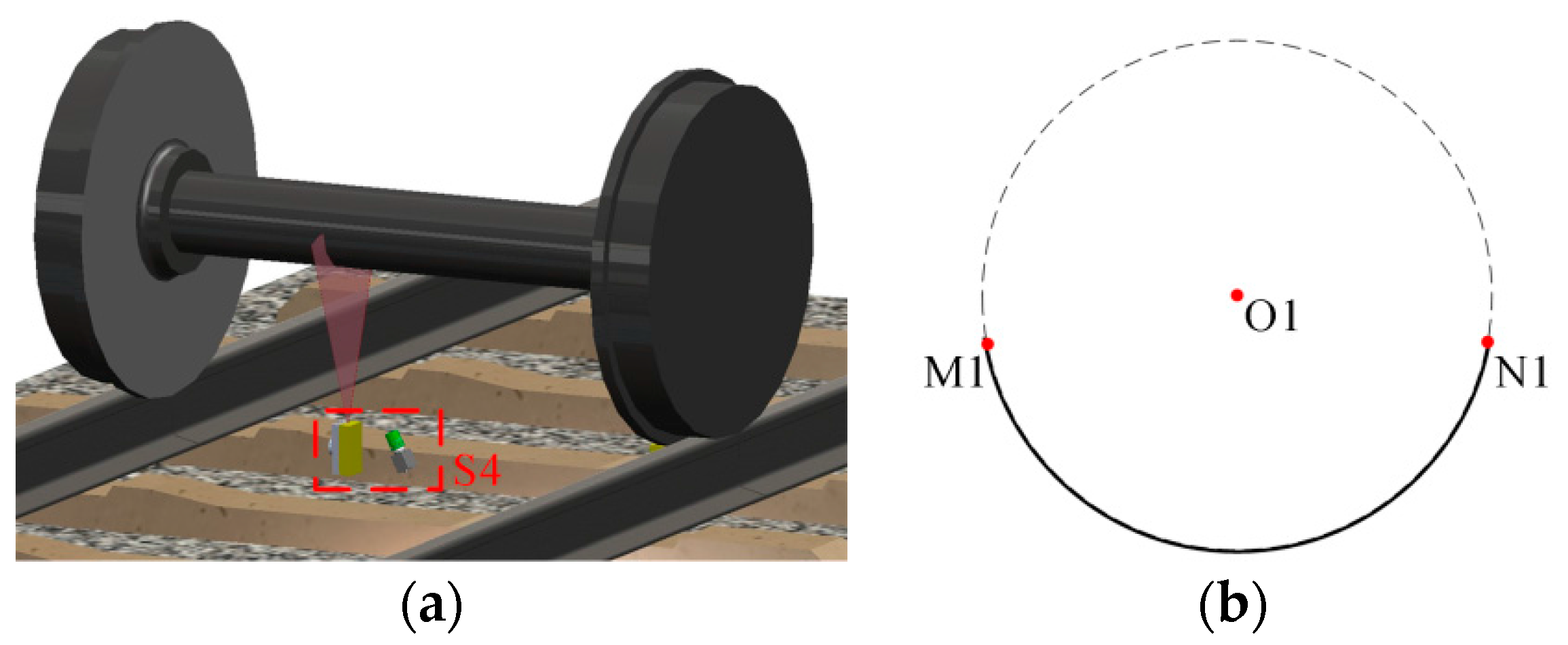
2.6.2. Determine the Axis of the Wheel Axle
2.6.3. Solve the Wheel Diameter
3. Simulation Analysis
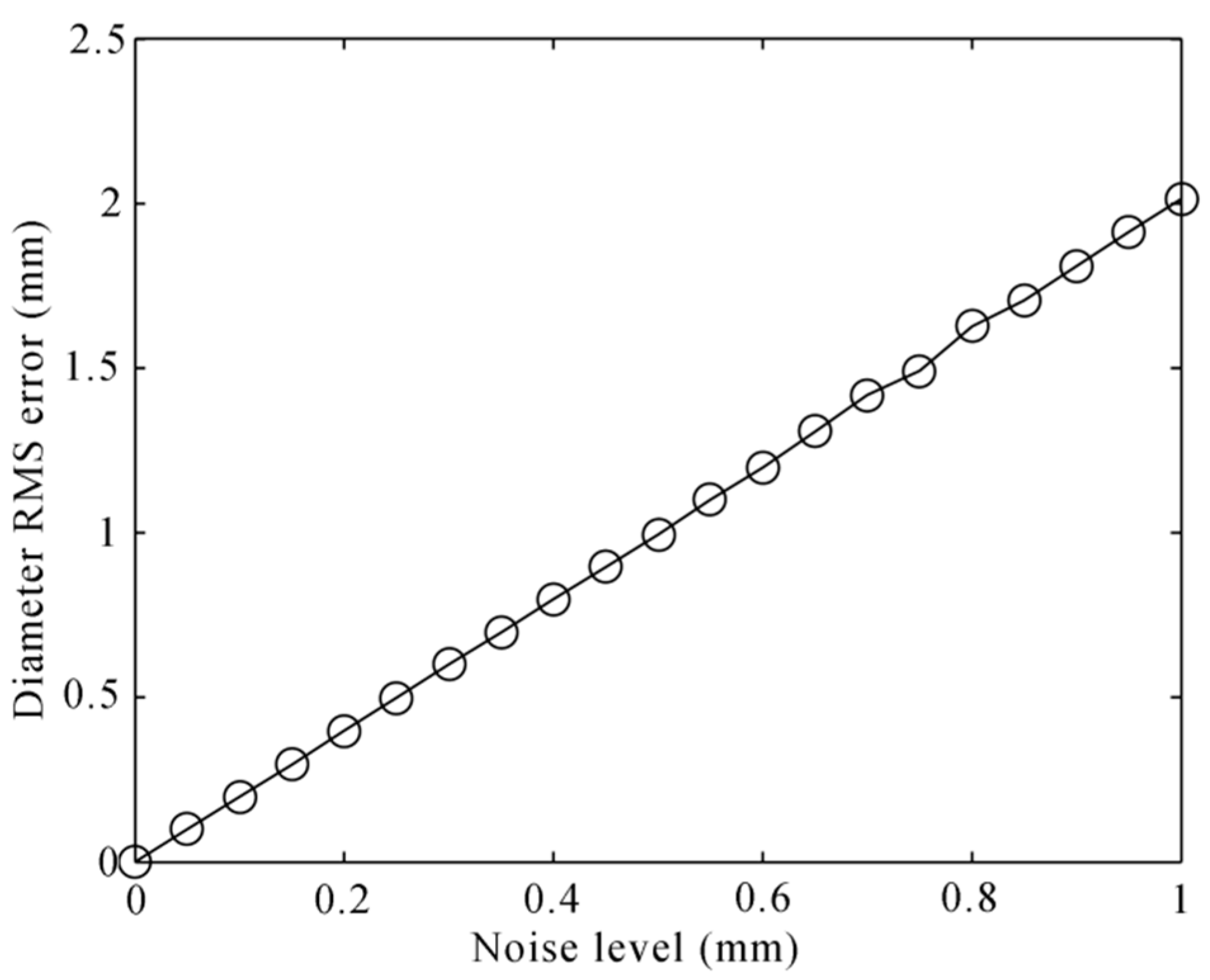
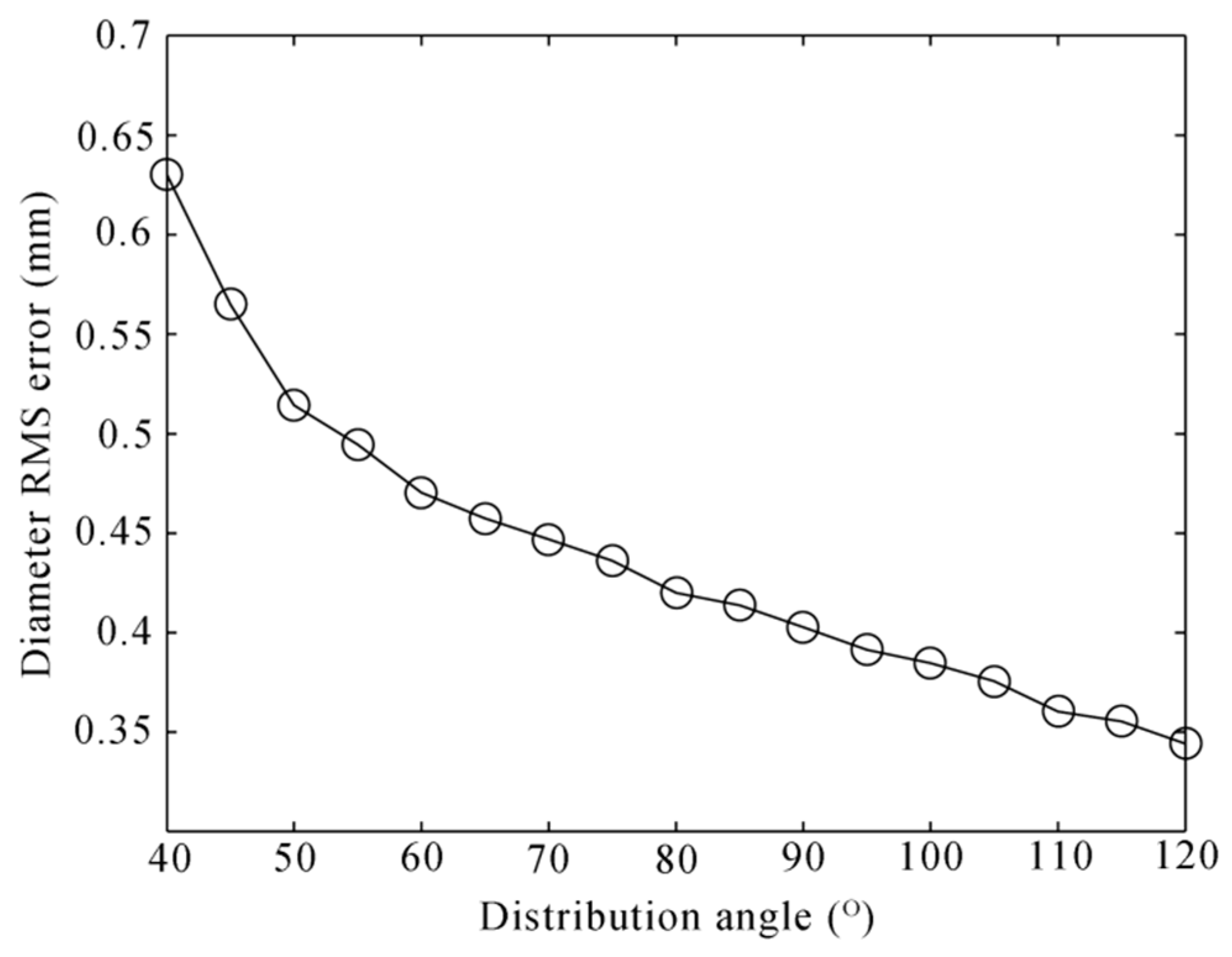
3.1. The Factor of the Measurement of the Structured-Light Sensors
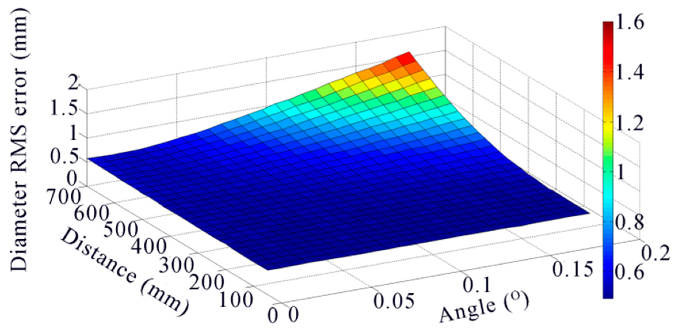
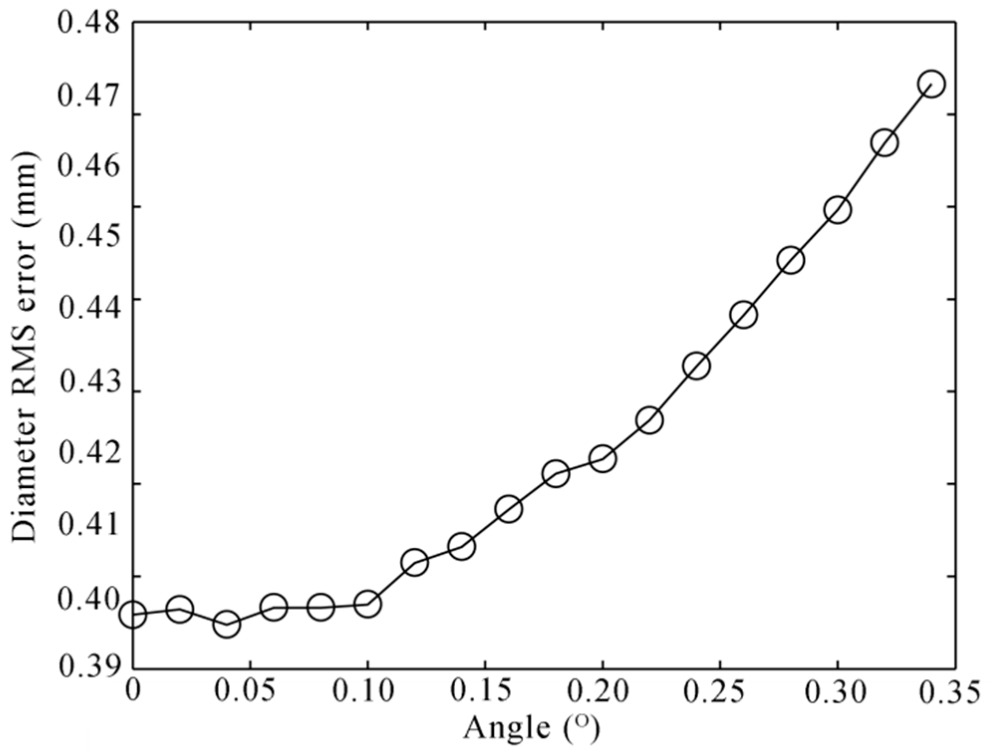
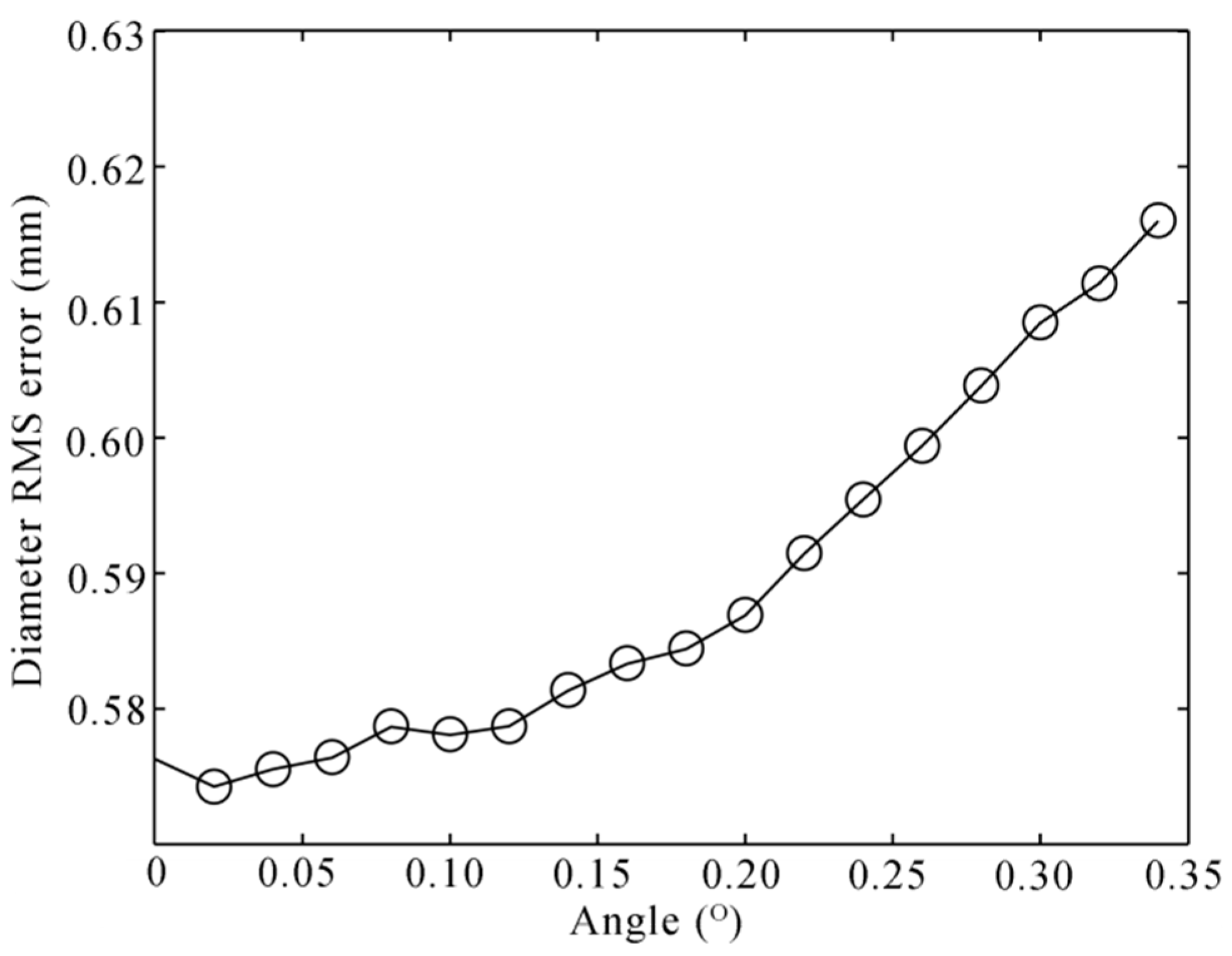
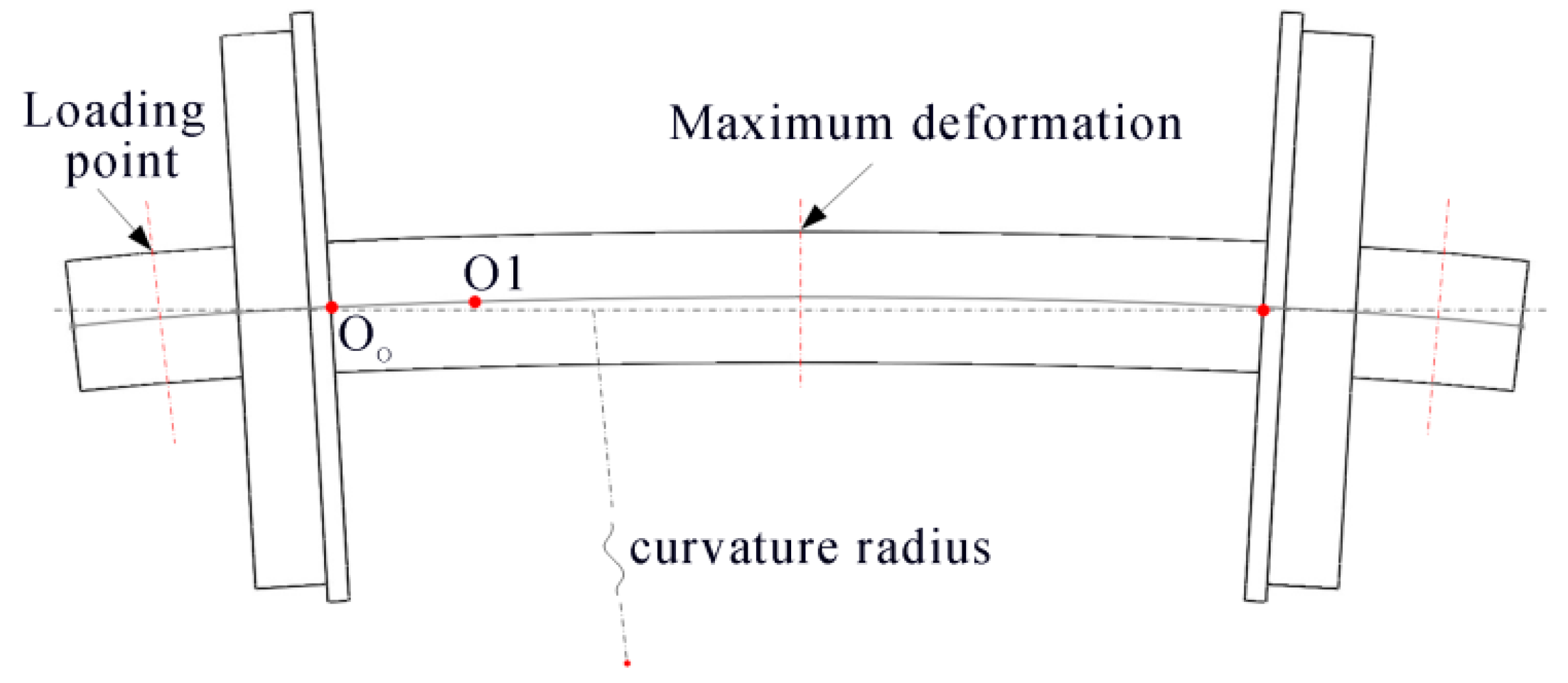
3.2. The Factor of the Deformation of the Wheelset Axle
3.3. The Factor of the Geometrical Error of the Wheelset Axle
4. Real Experiment
4.1. Static Experiment
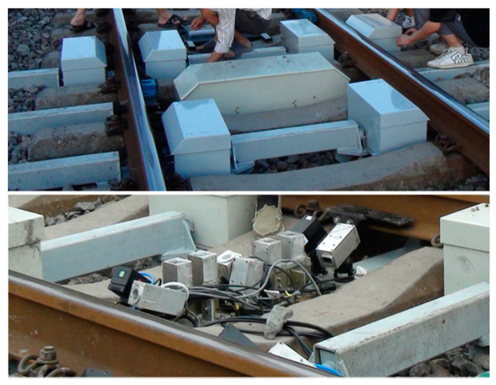
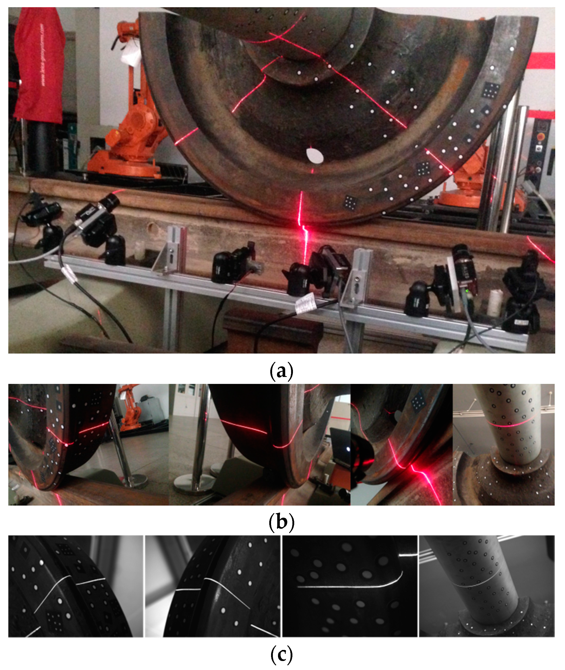
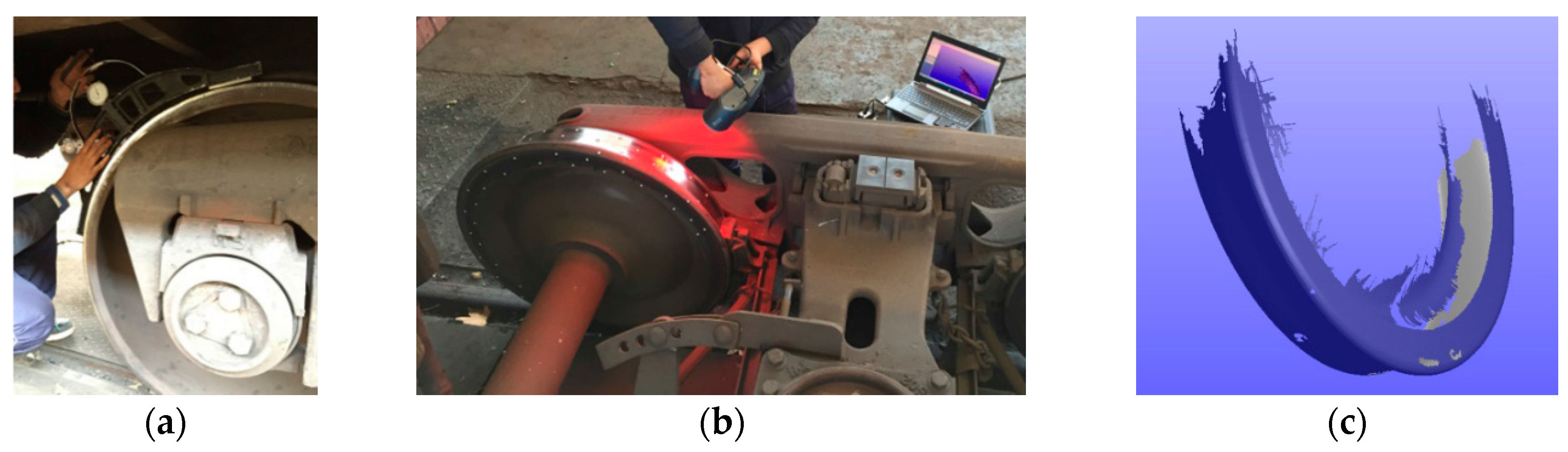
4.2. Dynamic Field Experiment
5. Conclusions
Acknowledgments
Author Contributions
Conflicts of Interest
Abbreviations
| LDS | laser displacement sensor |
| CCD | charge coupled device |
| CCF | camera coordinate frame |
| ICF | image coordinate frame |
| WCF | world coordinate frame |
| FOV | field of view |
| RMS | root mean square |
References
- Feng, Q.B.; Chen, S.Q. A new method for automatically measuring geometric parameters of wheel-sets by laser. Proc. SPIE 2003, 5253, 110–113. [Google Scholar]
- Wu, K.H.; Zhang, J.H.; Yan, K. Online measuring method of the wheel set wear based on CCD and image processing. Proc. SPIE 2005, 5633, 409–415. [Google Scholar]
- Mian, Z.F.; Hubin, T. Meth Method and System for Contact-less Measurement of Railroad Wheel Characteristics. U.S. Patent 5636026, 3 June 1997. [Google Scholar]
- Zhang, Z.F.; Lu, C.; Zhang, F.Z.; Ren, Y.F.; Yang, K.; Su, Z. A novel method for non-contact measuring diameter parameters of wheelset based on wavelet analysis. Optik 2012, 123, 433–438. [Google Scholar] [CrossRef]
- Gao, Y.; Feng, Q.B.; Cui, J.Y. A simple method for dynamically measuring the diameters of train wheels using a one-dimensional laser displacement transducer. Opt. Laser. Eng. 2014, 53, 158–163. [Google Scholar] [CrossRef]
- Wu, K.H.; Chen, J. Dynamic measurement for wheel diameter of train based on high-speed ccd and laser displacement sensors. Sens. Lett. 2011, 9, 2099–2103. [Google Scholar] [CrossRef]
- Sanchez-Revuelta, A.L.; Gömez, C.G. Installation and process for measuring rolling parameters by means of artificial vision on wheels of railway vehicles. U.S. Patent 5808906, 15 September 1998. [Google Scholar]
- Gao, Y.; Shao, S.Y.; Feng, Q.B. A new method for dynamically measuring diameters of train wheels using line structured light visual sensor. In Proceedings of the Symposium on Photonics & Optoelectronics, Shanghai, China, 21–23 May 2012; pp. 1–4.
- MERMEC Group. “Wheel Profile and Diameter”. Available online: http://www.mermecgroup.com/diagnosticsolutions/trainmonitoring/87/1/wheelprofile‑and‑diameter.php (accessed on 15 January 2016).
- IEM Inc. “Wheel profile system”. Available online: http://www.iem.net/products?id=150 (accessed on 15 January 2016).
- KLD Labs, Inc. “Wheel profile measurement”. Available online: http://www.kldlabs.com/index.php?s=wheel+profile+measurement (accessed on 15 January 2016).
- Gong, Z.; Sun, J.H.; Zhang, G.J. Dynamic structured-light measurement for wheel diameter based on the cycloid constraint. Appl. Opt. 2016, 55, 198–207. [Google Scholar] [CrossRef] [PubMed]
- Zhang, Z.Y. A flexible new technique for camera calibration. IEEE Trans. Pattern Anal. Mach. Intell. 2000, 22, 1330–1334. [Google Scholar] [CrossRef]
- Sun, J.H.; Zhang, G.J.; Liu, Q.Z.; Yang, Z. Universal method for calibrating structured-light vision sensor on the spot. J. Mech. Eng. 2009, 45, 174–177. [Google Scholar] [CrossRef]
- Esquivel, S.; Woelk, F.; Koch, R. Calibration of a multi-camera rig from non-overlapping views. Lect. Notes Comput. Sci. 2007, 4713, 82–91. [Google Scholar]
- Lebraly, P.; Deymier, C.; Ait-Aider, O.; Royer, E.; Dhome, M. Flexible extrinsic calibration of non-overlapping cameras using a planar mirror: Application to vision-based robotics. IEEE Int. Conf. Int. Robot Syst. 2010, 25, 5640–5647. [Google Scholar]
- Kazik, T.; Kneip, L.; Nikolic, J.; Pollefeys, M.; Siegwart, R. Real-time 6d stereo visual odometry with non-overlapping fields of view. IEEE Proc. CVPR 2012, 157, 1529–1536. [Google Scholar]
- Steger, C. An unbiased detector of curvilinear structures. IEEE Trans. Pattern Anal. Mach. Intell. 1998, 20, 113–125. [Google Scholar] [CrossRef]
- Chen, X.; Zhang, G.J.; Sun, J.H. An efficient and accurate method for real-time processing of light stripe images. Adv. Mech. Eng. 2013, 456927. [Google Scholar] [CrossRef]
- British Standard. Railway applications. Wheelsets and Bogies. Non Powered Axles. Design Method, BS EN 13103. 2009.
- British Standard. Railway applications. Wheelsets and Bogies. Axles. Product Requirements, BS EN 13261. 2009.
- Chinese Standard. Axles for railway cars. Types and Basic Dimensions, TB/T 3169-2007. 2007.


| Feature | Coordinate/Equation | Fitting Error |
|---|---|---|
| E1 | (148.31, 535.75, 471.05) | / |
| E2 | (−31.09, −0.84, 291.13) | / |
| C1 | (181.36, 565.43, 425.41) | / |
| C2 | (−11.36, −13.69, 232.34) | / |
| C3 | (−12.85, 343.45, 246.90) | / |
| O1 | (477.62, 165.72, 267.44) | / |
| Rim plane | 0.65345x + 0.035194y − 0.756148z − 170.55372 = 0 | 0.0031 |
| Oo | (290.51, 155.71, 483.85) | 0.010 |
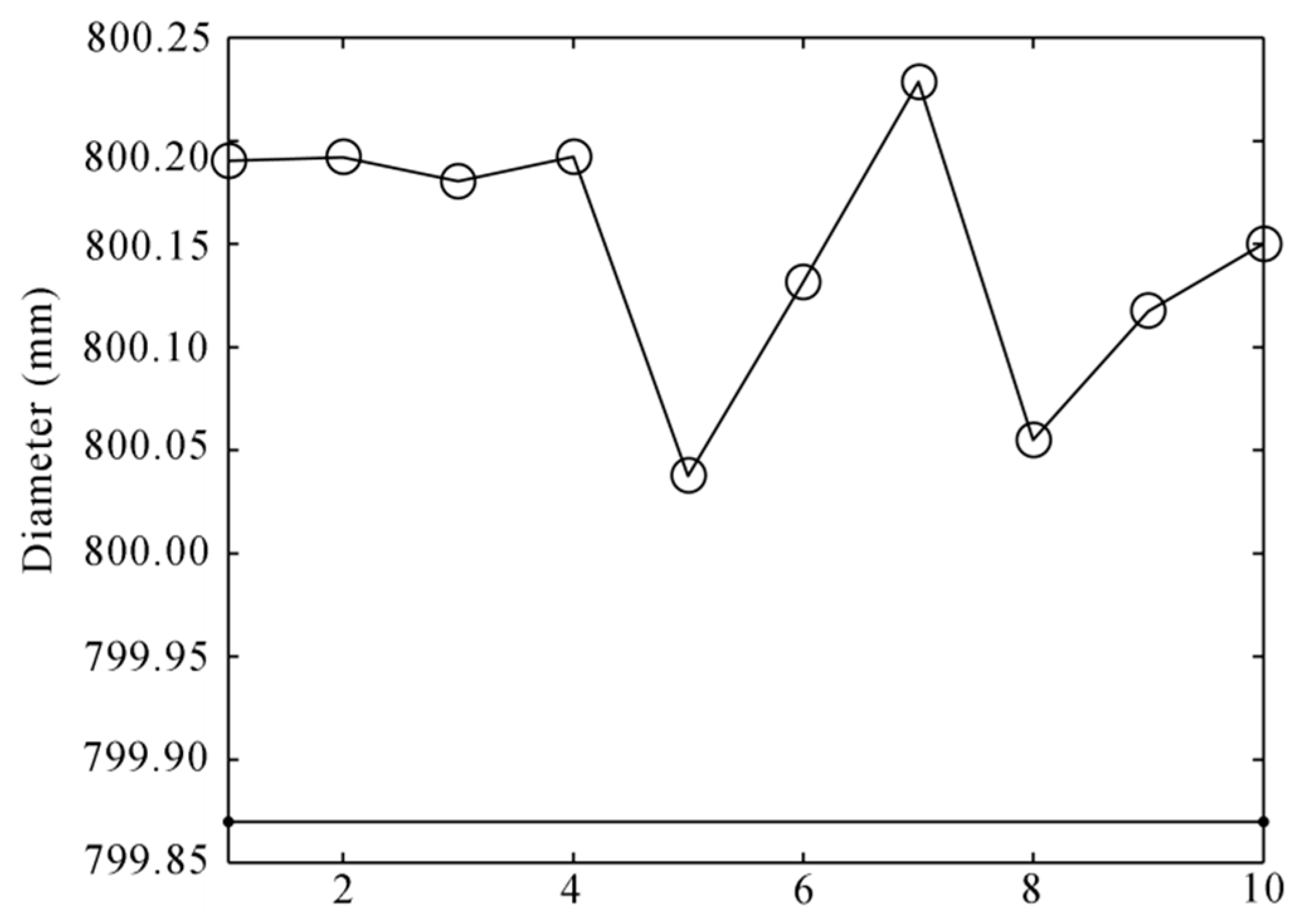
| Measurement Result | True-Value | Error |
|---|---|---|
| 800.15 | 799.87 | 0.28 |
| Vehicle ID (Speed) | Wheel Num. | 3D Scanner Result | System Result | Error |
|---|---|---|---|---|
| 4840409 (76 km/h) | 1 | 828.68 | 828.34 | 0.34 |
| 2 | 825.38 | 825.25 | 0.13 |
© 2016 by the authors; licensee MDPI, Basel, Switzerland. This article is an open access article distributed under the terms and conditions of the Creative Commons Attribution (CC-BY) license (http://creativecommons.org/licenses/by/4.0/).
Share and Cite
Gong, Z.; Sun, J.; Zhang, G. Dynamic Measurement for the Diameter of A Train Wheel Based on Structured-Light Vision. Sensors 2016, 16, 564. https://doi.org/10.3390/s16040564
Gong Z, Sun J, Zhang G. Dynamic Measurement for the Diameter of A Train Wheel Based on Structured-Light Vision. Sensors. 2016; 16(4):564. https://doi.org/10.3390/s16040564
Chicago/Turabian StyleGong, Zheng, Junhua Sun, and Guangjun Zhang. 2016. "Dynamic Measurement for the Diameter of A Train Wheel Based on Structured-Light Vision" Sensors 16, no. 4: 564. https://doi.org/10.3390/s16040564
APA StyleGong, Z., Sun, J., & Zhang, G. (2016). Dynamic Measurement for the Diameter of A Train Wheel Based on Structured-Light Vision. Sensors, 16(4), 564. https://doi.org/10.3390/s16040564