
GNSS Precise Kinematic Positioning for Multiple Kinematic Stations Based on A Priori Distance Constraints

 ,
,  , ,
, ,
Abstract
:1. Introduction
2. Kinematic Positioning Based on A Priori Distance Constraints
2.1. Classic Kalman Filter
2.2. The Distance between Two Kinematic GNSS Antennas
2.3. The A Priori Distance Constraints
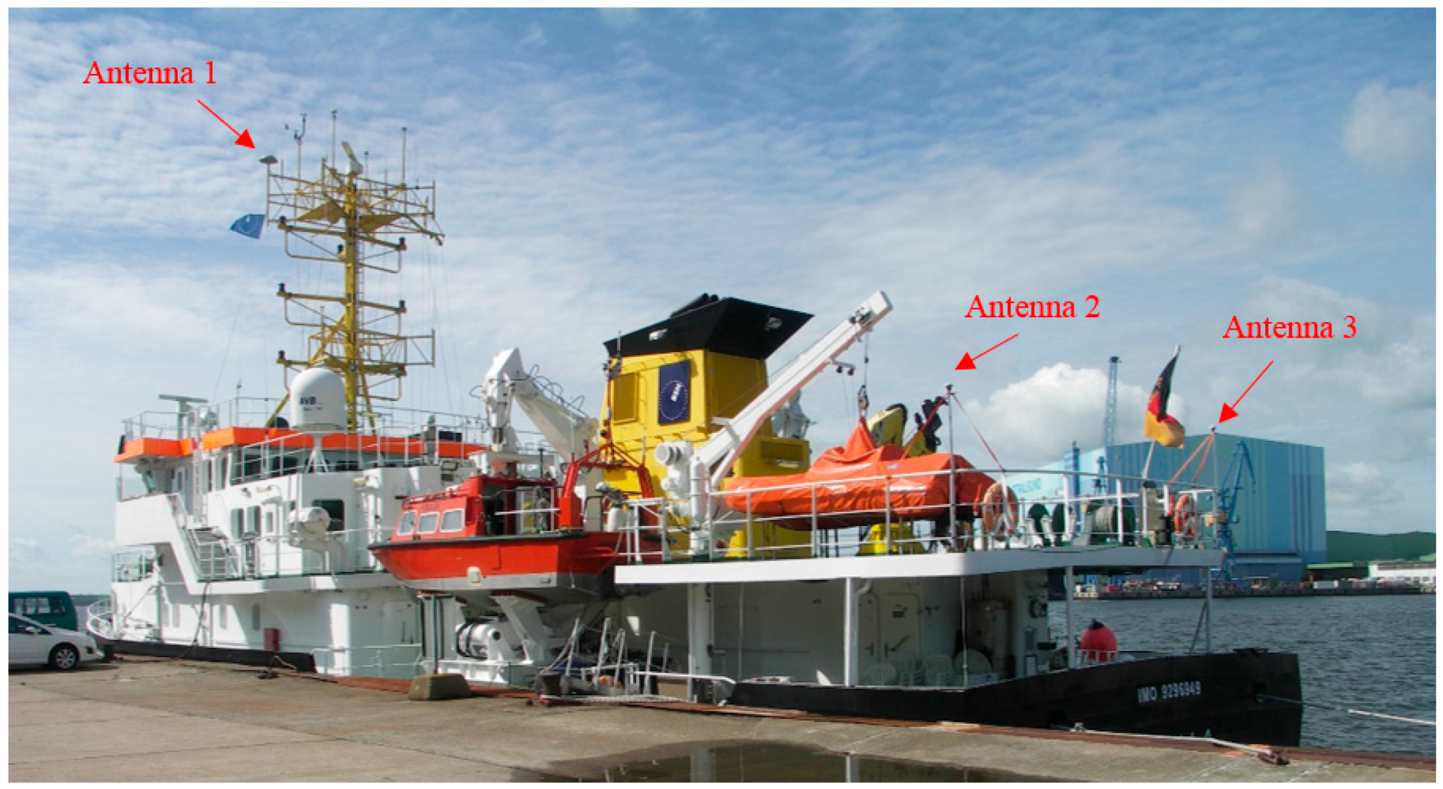
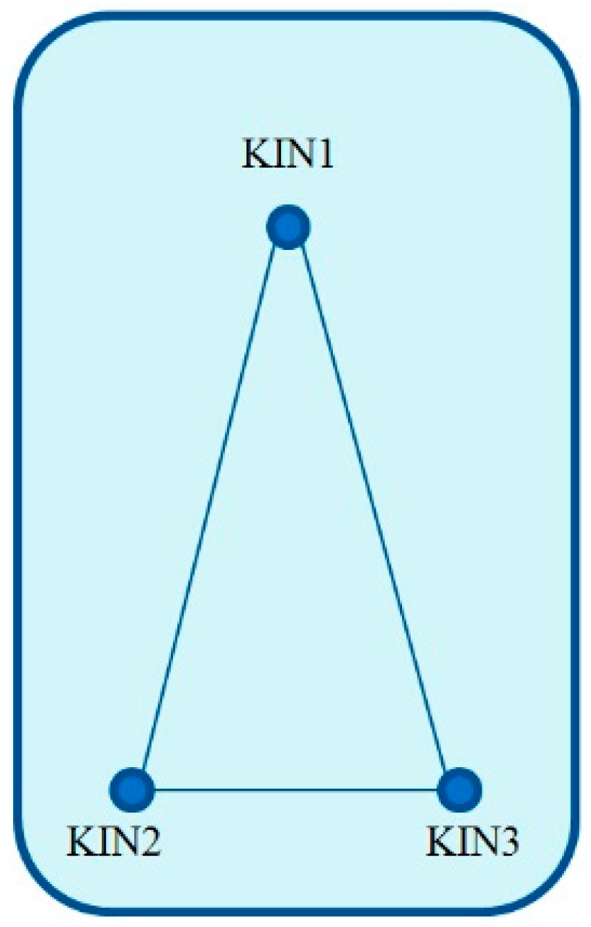
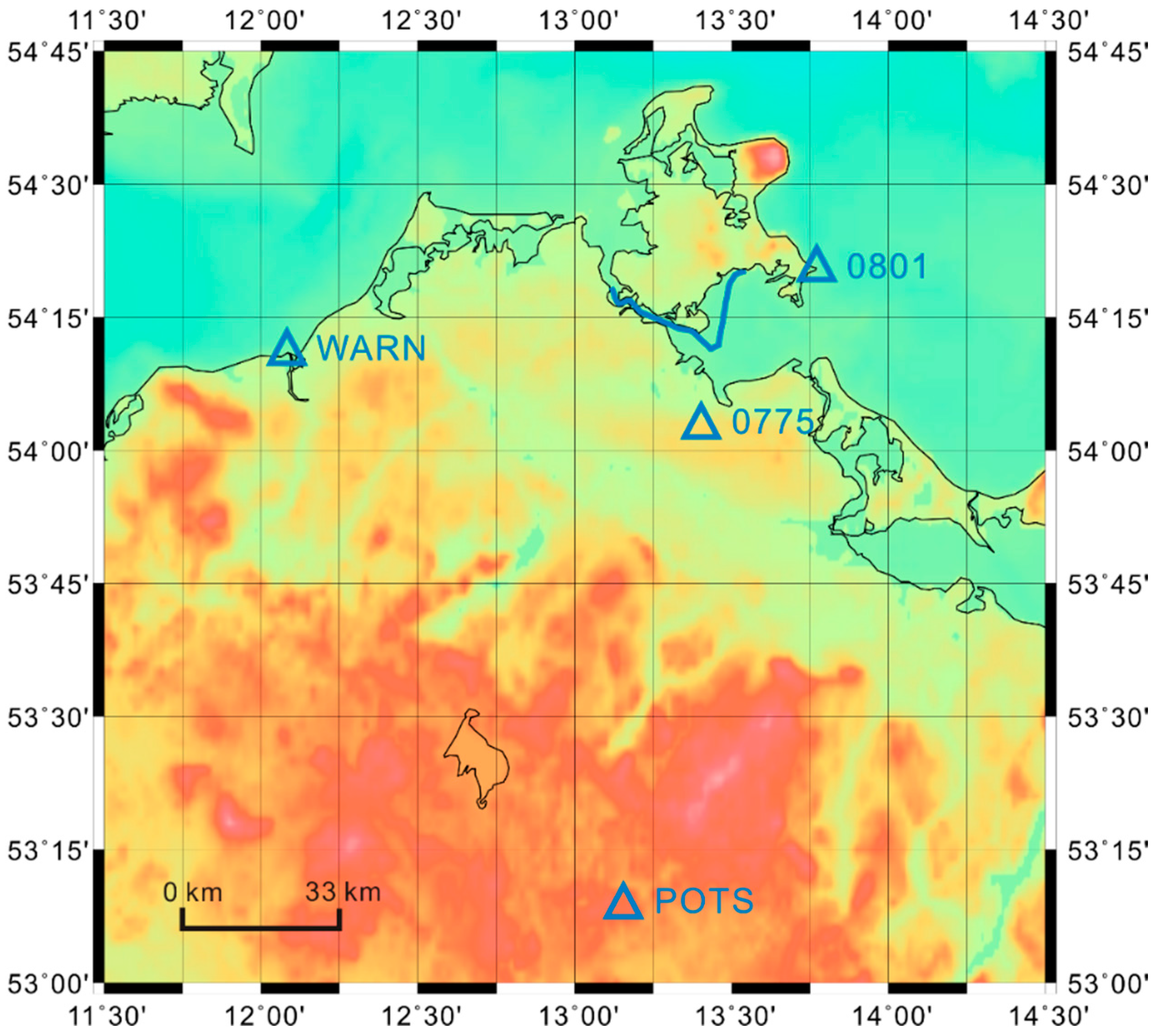
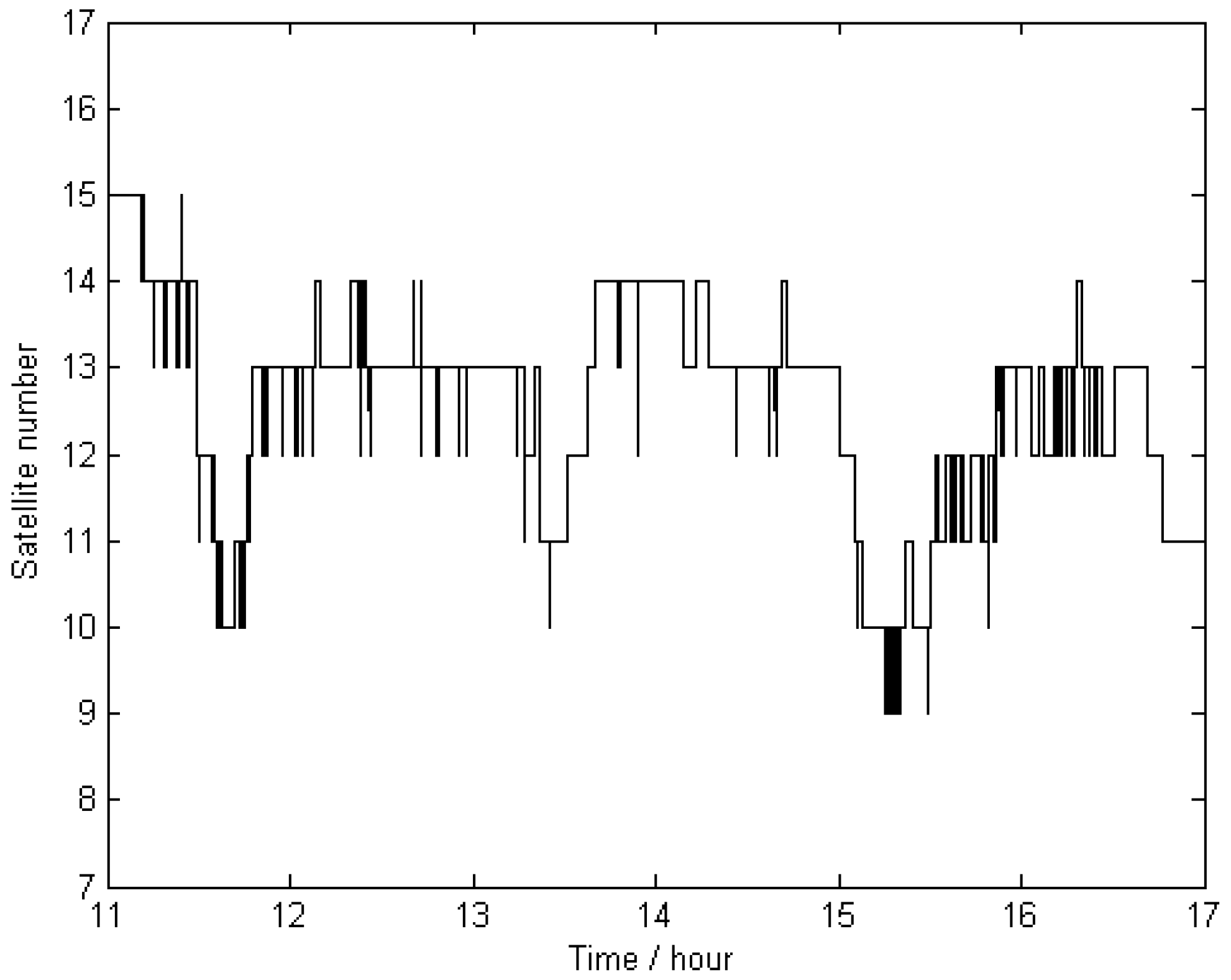
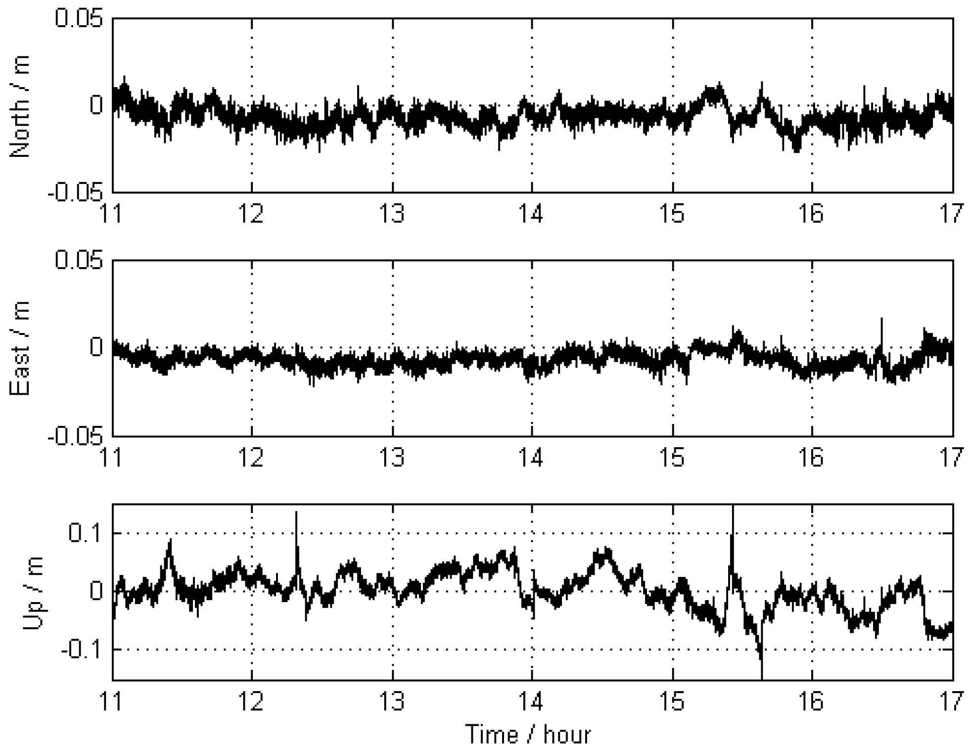
3. Experiment and Analysis
4. Conclusions
Acknowledgments
Author Contributions
Conflicts of Interest
References
- Kwon, J.H.; Jekeli, C.A. New approach for airborne vector gravimetry using GPS/INS. J. Geod. 2001, 74, 690–700. [Google Scholar] [CrossRef]
- Hein, G.W. Progress in airborne gravimetry: Solved, open and critical problems. In Proceedings of the IAG Symposium on Airborne Gravity Field Determination, IUGG XXI General Assembly, Boulder, CO, USA, 2–14 July 1995; pp. 3–11.
- Forsberg, R.; Olesen, A.V. Airborne Gravity Field Determination. In Sciences of Geodesy-I Advances and Future Directions; Xu, G., Ed.; Springer: Heidelberg, Germany; London, UK; New York, NY, USA, 2010; pp. 83–104. [Google Scholar]
- Hannah, J. Airborne Gravimetry: A Status Report; Department of Surveying, University of Otago: Dunedin, New Zealand, 2001. [Google Scholar]
- Petrovic, S.; Barthelmes, F.; Pflug, H. Airborne and Shipborne Gravimetry at GFZ with Emphasis on the GEOHALO project. In IAG 150 Years; Rizos, C., Willis, P., Eds.; Springer International Publishing: Potsdam, Germany, 2016. [Google Scholar]
- Barzaghi, R.; Albertella, A.; Carrion, D.; Barthelmes, F.; Petrovic, S.; Scheinert, M. Testing airborne gravity data in the large-scale area of Italy and adjacent seas. In IAG 150 Years; Rizos, C., Willis, P., Eds.; Springer International Publishing: Potsdam, Germany, 2016. [Google Scholar]
- He, K.; Xu, G.; Xu, T.; Flechtner, F. GNSS navigation and positioning for the GEOHALO experiment in Italy. GPS Solut. 2016, 20, 215–224. [Google Scholar] [CrossRef]
- Schwarz, K.P.; Cannon, M.E.; Wong, R.V.C. A comparison of GPS kinematic models for the determination of position and velocity along a trajectory. Manuscr. Geod. 1989, 14, 345–353. [Google Scholar]
- Abdel-salam, M.A. Precise Point Positioning Using Un-differenced Code and Carrier Phase Observations. Ph.D. Thesis, University of Calgary, Calgary, AB, Canada, 9 September 2005. [Google Scholar]
- Yang, Y. Adaptively robust kalman filters with applications in navigation. In Sciences of Geodesy-I Advances and Future Directions; Xu, G., Ed.; Springer: Heidelberg, Germany, 2010; pp. 49–82. [Google Scholar]
- Kalman, R.E. A new approach to linear filtering and prediction problems. J. Fluids Eng. 1960, 82, 35–45. [Google Scholar] [CrossRef]
- Kalman, R.E.; Bucy, R.S. New results in linear filtering and prediction theory. J. Fluids Eng. 1961, 83, 95–108. [Google Scholar] [CrossRef]
- Huang, G.; Zhang, Q. Real-time estimation of satellite clock offset using adaptively robust Kalman filter with classified adaptive factors. GPS Solut. 2012, 16, 531–539. [Google Scholar] [CrossRef]
- Yang, Y.; Gao, W.; Zhang, X. Robust Kalman filtering with constraints: A case study for integrated navigation. J. Geod. 2010, 84, 373–381. [Google Scholar] [CrossRef]
- Simon, D.; Chia, T.L. Kalman filtering with state equality constraints. IEEE Trans. Aerosp. Electron. Syst. 2002, 38, 128–136. [Google Scholar] [CrossRef]
- Ko, S.; Bitmead, R.R. State estimation for linear systems with state equality constraints. Automatica. 2007, 43, 1363–1368. [Google Scholar] [CrossRef]
- Julier, S.J.; LaViola, J.J. On Kalman filtering with nonlinear equality constraints. IEEE Trans. Signal Process. 2007, 55, 2774–2784. [Google Scholar] [CrossRef]
- Doran, H.E. Constraining Kalman filter and smoothing estimates to satisfy time-varying restrictions. Rev. Econ. Stat. 1992, 74, 568–572. [Google Scholar] [CrossRef]
- Leick, A.; Rapoport, L.; Tatarnikov, D. GPS Satellite Surveying; John Wiley & Sons: Hoboken, NJ, USA, 2015. [Google Scholar]
- Marreiros, J.P.R. Kinematic GNSS Precise Point Positioning: Aplication to Marine Platforms. Ph.D. Thesis, University of Porto, Porto, Portugal, 6 June 2013. [Google Scholar]
- Colombo, O.L.; Sutter, A.W.; Evans, A.G. Evaluation of precise, kinematic GPS point positioning. In Proceedings of the 17th International Technical Meeting of the Satellite Division of The Institute of Navigation (ION GNSS 2004), Long Beach, CA, USA, 21 September 2004; pp. 1423–1430.
- He, K. GNSS Kinematic Position and Velocity Determination for Airborne Gravimetry. Ph.D. Thesis, GFZ-German Research Centre for Geosciences, Potsdam, Germany, 1 April 2015. [Google Scholar]
- Zhang, B. Determination of un-differenced atmospheric delays for network-based RTK. In Proceedings of the 22nd International Technical Meeting of The Satellite Division of the Institute of Navigation (ION GNSS 2009), Savannah, GA, USA, 22–25 September 2009; pp. 2727–2738.
- Xu, T.; He, K.; Xu, G. Orbit determination and thrust force modeling for a maneuvered GEO satellite using two-way adaptive Kalman filtering. Sci. China Phys. Mech. Astron. 2012, 55, 738–743. [Google Scholar] [CrossRef]
- Genrich, J.F.; Bock, Y. Rapid resolution of crustal motion at short ranges with the Global Positioning System. J. Geop. Res. Solid Earth 1992, 97, 3261–3269. [Google Scholar] [CrossRef]
- Li, B.; Shen, Y.; Feng, Y.; Gao, W.; Yang, L. GNSS ambiguity resolution with controllable failure rate for long baseline network RTK. J. Geod. 2014, 88, 99–112. [Google Scholar] [CrossRef]
- Wielgosz, P.; Kashani, I.; Grejner-Brzezinska, D. Analysis of long-range network RTK during a severe ionospheric storm. J. Geod. 2005, 79, 524–531. [Google Scholar] [CrossRef]


| Station Name | Receiver Type | Antenna Type | With Radome |
|---|---|---|---|
| KIN1 | JAVAD TRE_G3TH DELTA | LEIAS10 | NONE |
| KIN3 | JAVAD TRE_G3TH DELTA | ACCG5ANT_42AT1 | NONE |
| 0801 | TPS NET-G3A | TPSCR.G3 | TPSH |
| 0775 | TPS NET-G3A | TPSCR.G3 | TPSH |
| WARN | JPS LEGACY | LEIAR25.R3 | LEIT |
| POTS | JAVAD TRE_G3TH DELTA | JAV_RINGANT_G3T | NONE |
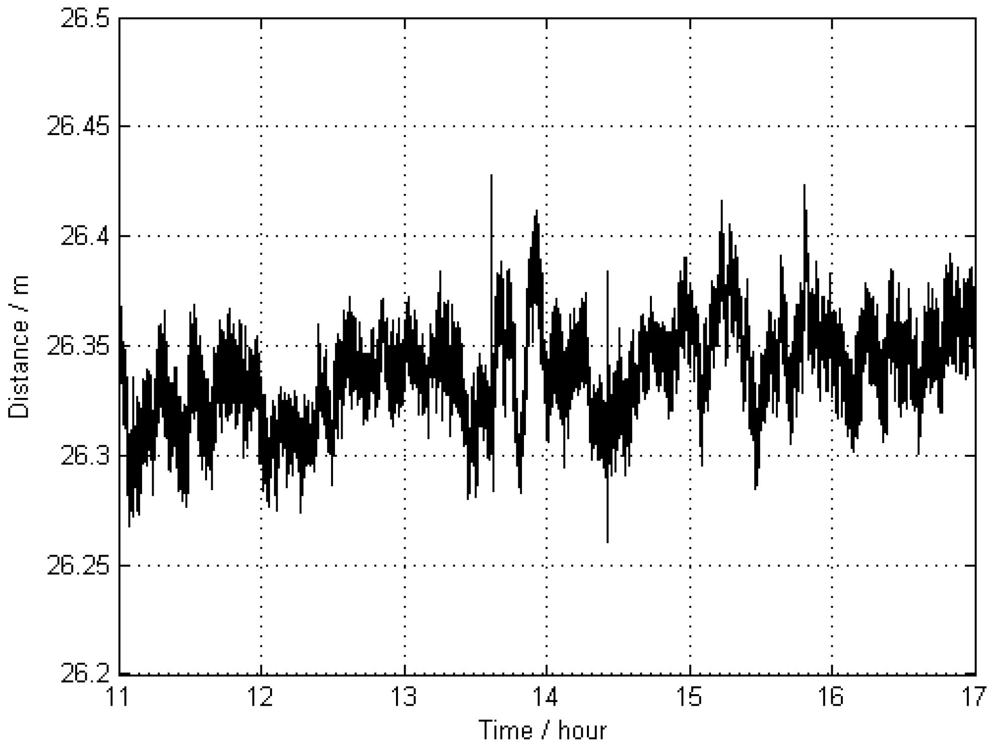
| Scheme | Reference Stations | Min | Max | Mean | STD |
|---|---|---|---|---|---|
| 1 | Nearby | 26.282 | 26.406 | 26.342 | 0.015 |
| 2 | Far away | 26.261 | 26.428 | 26.338 | 0.022 |
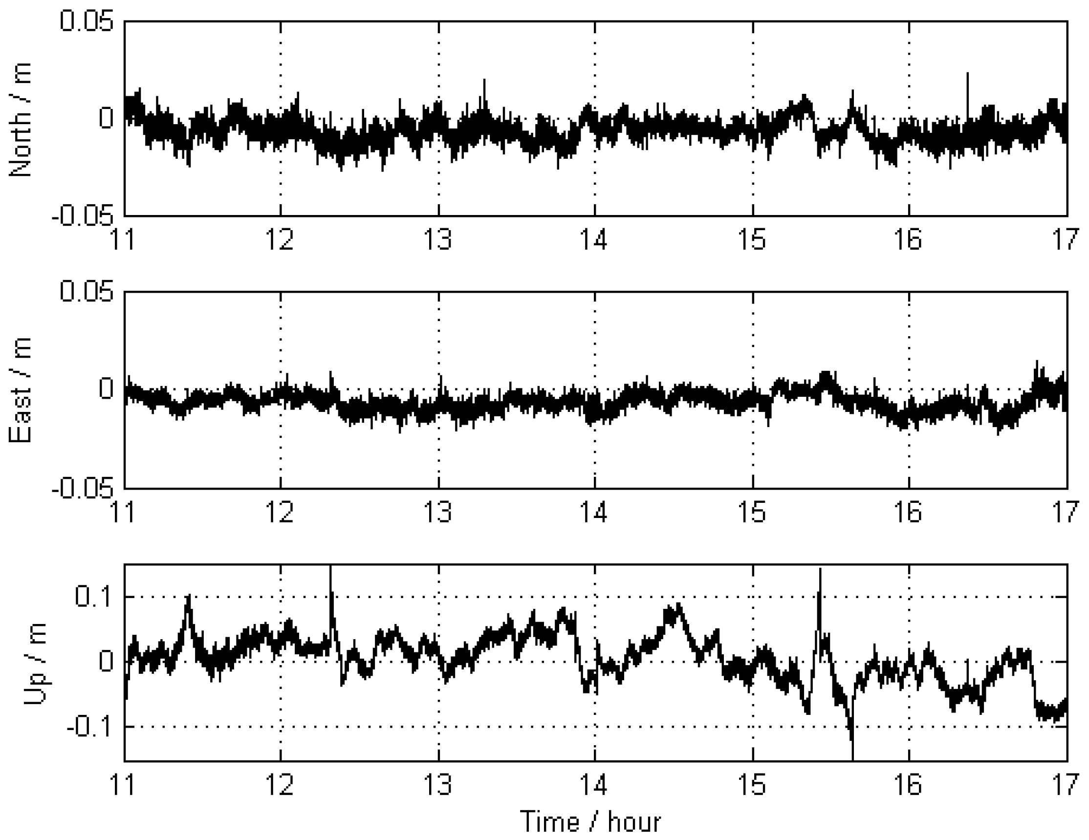
| Scheme | Direction | Min | Max | Mean | RMS |
|---|---|---|---|---|---|
| 2 vs. 1 | North | –27.0 | 23.0 | –6.4 | 5.8 |
| East | –23.5 | 14.8 | –6.4 | 4.5 | |
| Up | –165.7 | 165.9 | 3.5 | 36.8 | |
| 3 vs. 1 | North | –27.7 | 15.8 | –6.4 | 5.8 |
| East | –21.6 | 16.4 | –6.6 | 4.2 | |
| Up | –161.6 | 145.4 | 0.0 | 33.1 |
© 2016 by the authors; licensee MDPI, Basel, Switzerland. This article is an open access article distributed under the terms and conditions of the Creative Commons by Attribution (CC-BY) license (http://creativecommons.org/licenses/by/4.0/).
Share and Cite
He, K.; Xu, T.; Förste, C.; Petrovic, S.; Barthelmes, F.; Jiang, N.; Flechtner, F. GNSS Precise Kinematic Positioning for Multiple Kinematic Stations Based on A Priori Distance Constraints. Sensors 2016, 16, 470. https://doi.org/10.3390/s16040470
He K, Xu T, Förste C, Petrovic S, Barthelmes F, Jiang N, Flechtner F. GNSS Precise Kinematic Positioning for Multiple Kinematic Stations Based on A Priori Distance Constraints. Sensors. 2016; 16(4):470. https://doi.org/10.3390/s16040470
Chicago/Turabian StyleHe, Kaifei, Tianhe Xu, Christoph Förste, Svetozar Petrovic, Franz Barthelmes, Nan Jiang, and Frank Flechtner. 2016. "GNSS Precise Kinematic Positioning for Multiple Kinematic Stations Based on A Priori Distance Constraints" Sensors 16, no. 4: 470. https://doi.org/10.3390/s16040470
APA StyleHe, K., Xu, T., Förste, C., Petrovic, S., Barthelmes, F., Jiang, N., & Flechtner, F. (2016). GNSS Precise Kinematic Positioning for Multiple Kinematic Stations Based on A Priori Distance Constraints. Sensors, 16(4), 470. https://doi.org/10.3390/s16040470