
Registration of Feature-Poor 3D Measurements from Fringe Projection


Abstract
:1. Introduction
2. Measurement and Registration of 3D Data
2.1. 3D Measurement for Surface Quality Inspection
2.1.1. Finding Corresponding Image Points
2.1.2. Camera Calibration
2.2. Registration of 3D Data
3. Texture-Based Registration Algorithm
- (a)
- Camera calibrationgives a mapping from a 3D point in the sensor coordinate system of measurement i to a corresponding camera image coordinate of camera c. Camera calibration is constant for each measurement i. Any model that matches this abstraction, can be considered. An example calibration model is given in Appendix. In the algorithm description below, we consider registration of two measurements , each taken with a stereo camera system .
- (b)
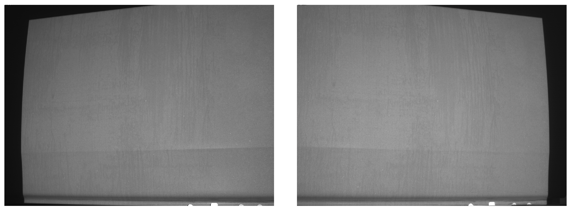
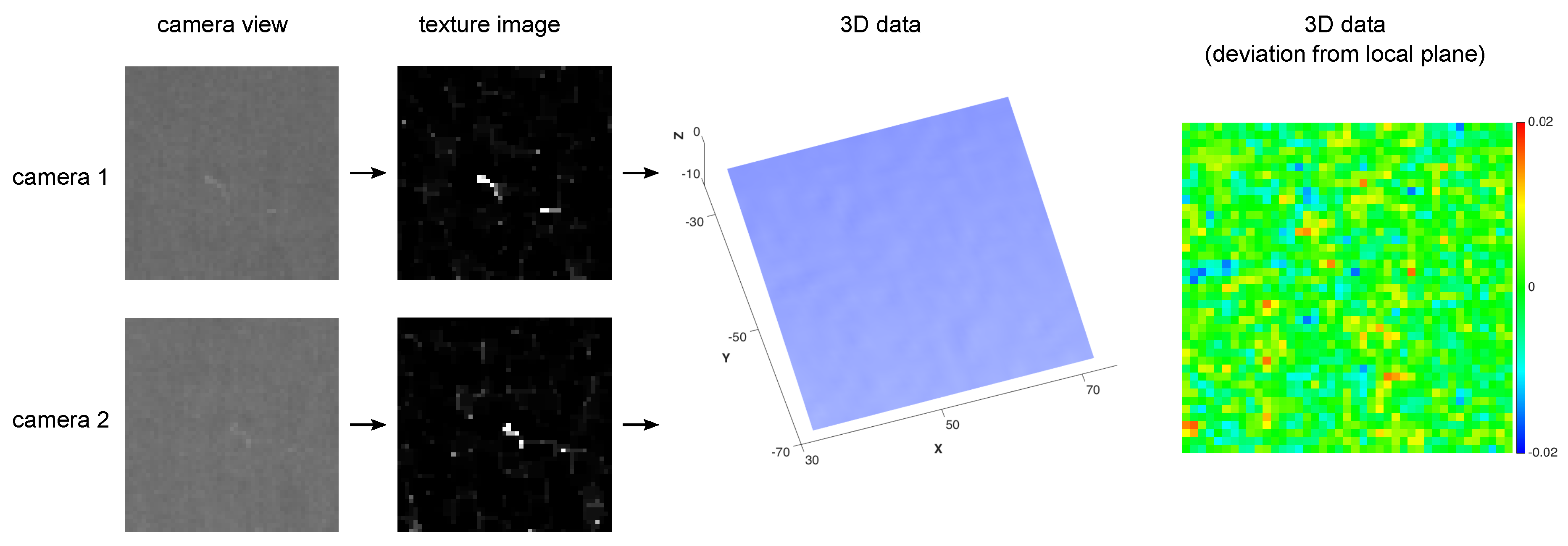
- Camera image (blank projection)the image typically is a matrix of (8-bit) integer gray scale values. Sub-pixel values for general image coordinates result from bilinear interpolation of the four neighbouring pixels’ values. Again, each measurement is indicated by index i and each camera is indicated by index c.
- (c)
- 3D point cloudwhere each 3D point results from triangulation of corresponding image points. Each measurement i may contain a different number of 3D points.
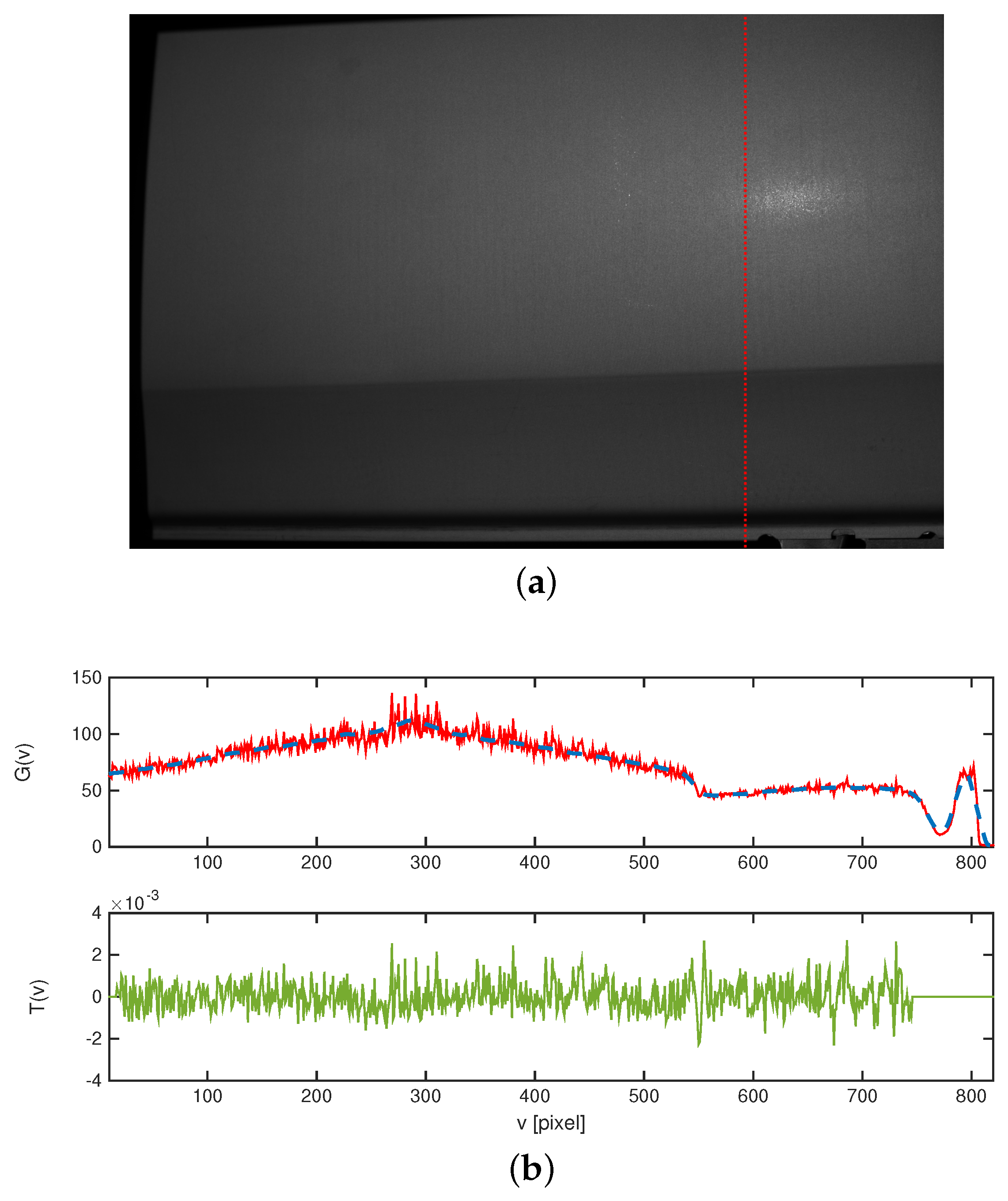
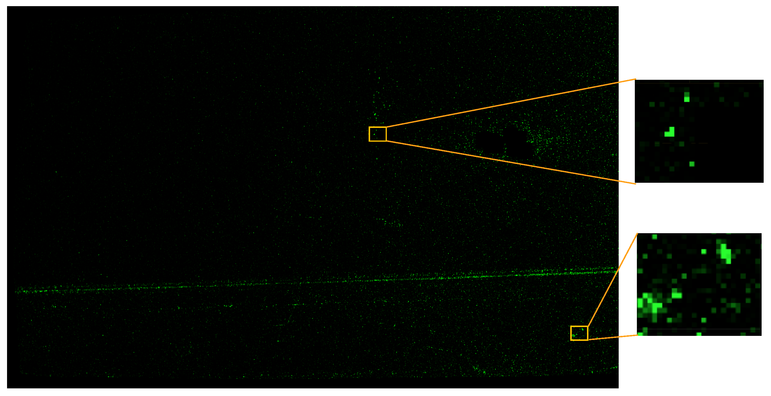
3.1. Texture Image
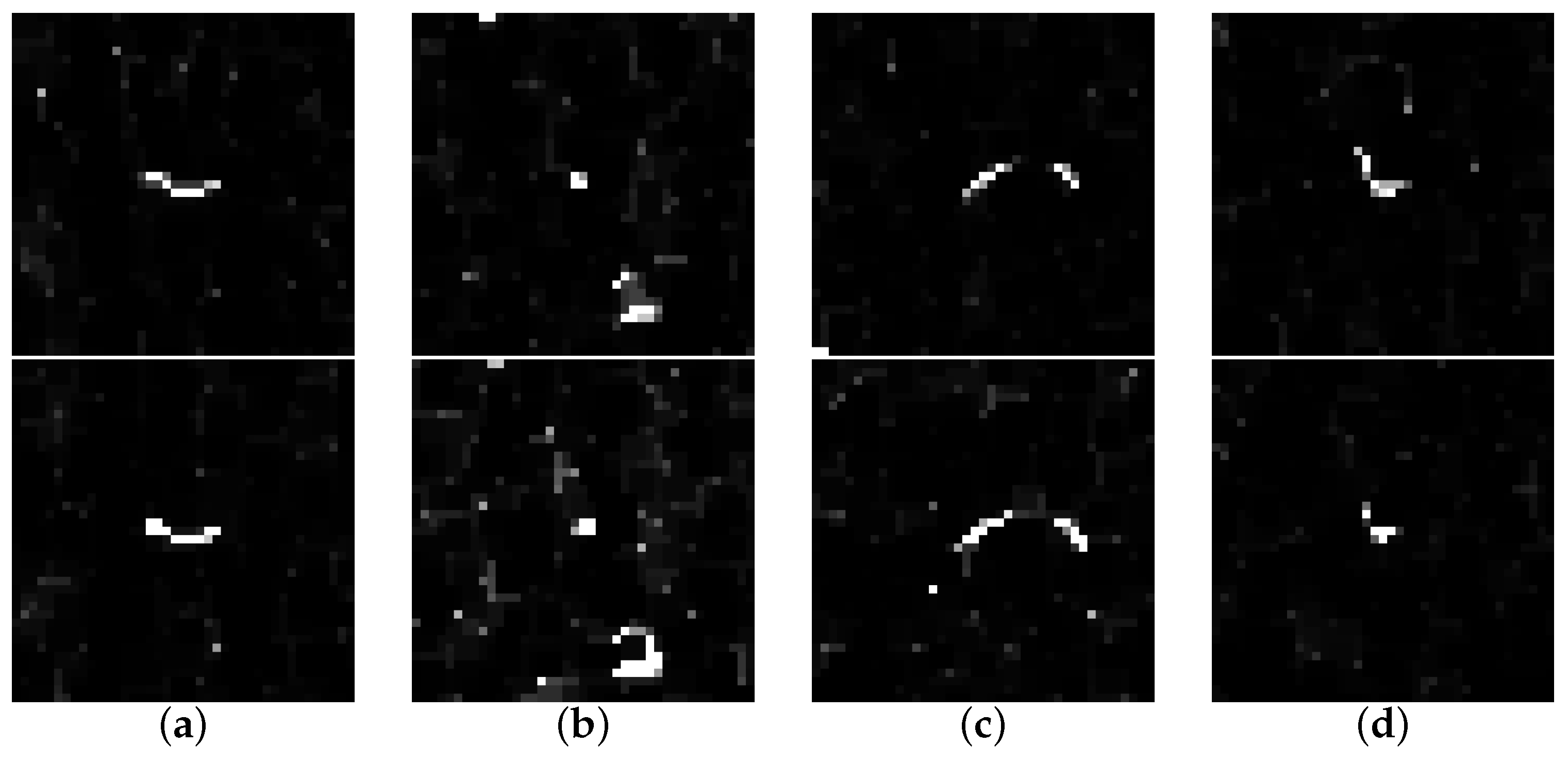
3.2. 2D Keypoints and Matching
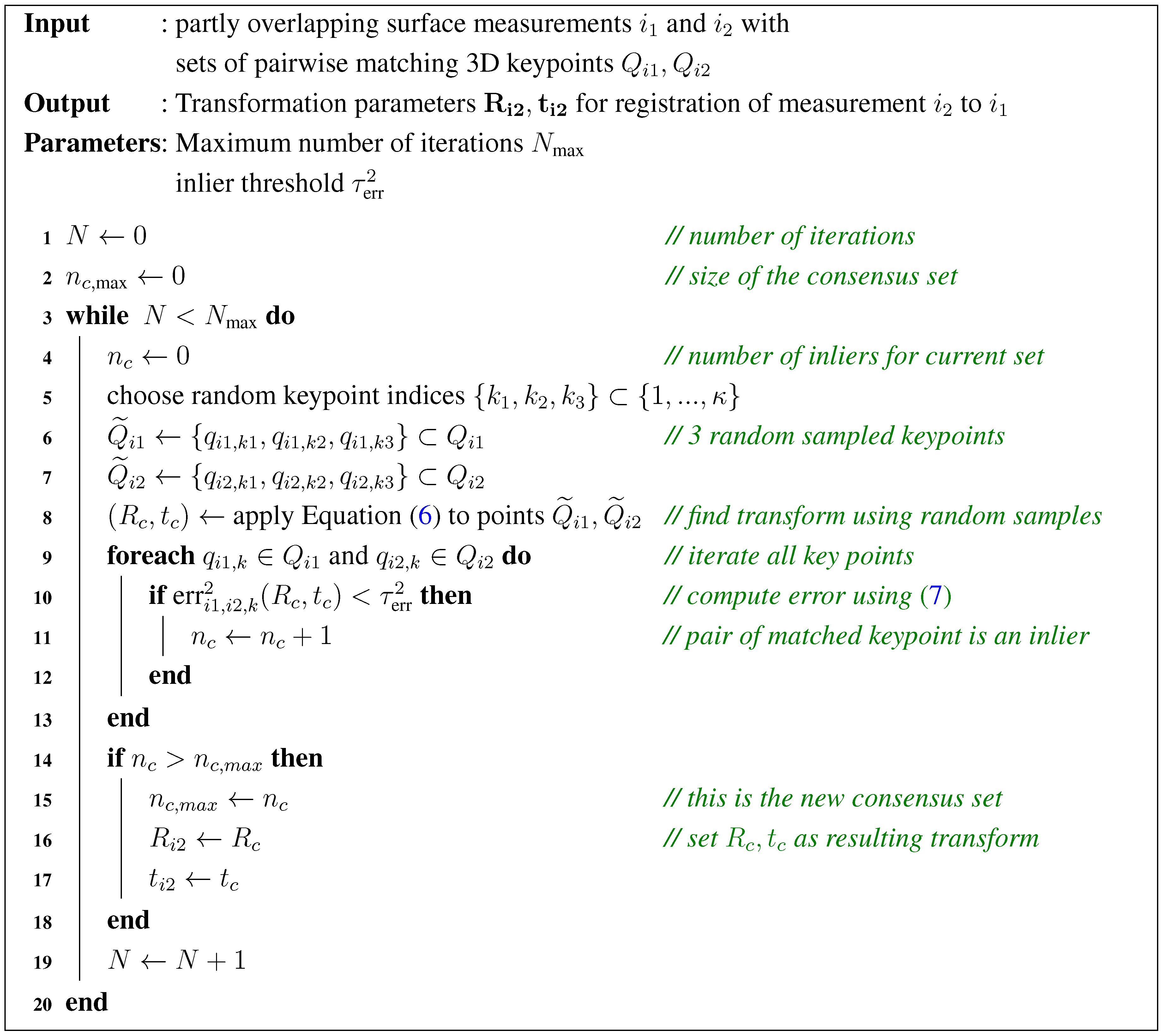
3.3. Estimation of 3D Parameters
4. Experimental Results and Discussion
5. Conclusions
Acknowledgments
- The authors would like to extend their sincere appreciation to the Deanship of Scientific Research at King Saud University for its funding of this International Research Group (IRG14-28).
- This work is part of a project funded by the German Federal Ministry for Economic Affairs and Energy (No. KF-3172302-WM4).
Author Contributions
Conflicts of Interest
Appendix
Camera Calibration Model
- External Calibration:
- 2D Projection:
- Radial Distortion:
References
- Denkena, B.; Berg, F.; Acker, W. Surface Inspection System for Large Sheet Metal Parts. Adv. Mater. Res. 2005, 6–8, 559–564. [Google Scholar] [CrossRef]
- Molleda, J.; Usamentiaga, R.; García, D.F.; Bulnes, F.G.; Espina, A.; Dieye, B.; Smith, L.N. An improved 3D imaging system for dimensional quality inspection of rolled products in the metal industry. Comput. Ind. 2013, 64, 1186–1200. [Google Scholar] [CrossRef]
- De la Fuente López, E.; Trespaderne, F.M. Inspection of stamped sheet metal car parts using a multiresolution image fusion technique. Comput. Vis. Syste. 2009, 5815, 345–353. [Google Scholar]
- Von Enzberg, S.; Al-Hamadi, A. A defect recognition system for automated inspection of non-rigid surfaces. In Proceedings of the International Conference on Pattern Recognition, Stockholm, Sweden, 24–28 August 2014; pp. 1812–1816.
- Newman, T.S.; Jain, A.K. A survey of automated visual inspection. Comput. Vis. Image Underst. 1995, 61, 231–262. [Google Scholar] [CrossRef]
- Rusinkiewicz, S.; Levoy, M. Efficient variants of the ICP algorithm. In Proceedings of the Third International Conference on 3-D Digital Imaging and Modeling, Montreal, QC, Canada, 28 May–1 June 2001; pp. 145–152.
- Chen, Y.; Medioni, G. Object modeling by registration of multiple range images. In Proceedings of the 1991 IEEE International Conference on Robotics and Automation, Sacramento, CA, USA, 9–11 April 1991; pp. 2724–2729.
- Ribo, M.; Brandner, M. State of the art on vision-based structured light systems for 3D measurements. In Proceedings of the International Workshop on Robotic Sensors: Robotic and Sensor Environments, Ottawa, ON, Canada, 30 September–1 October 2005; pp. 2–6.
- Salvi, J.; Armangué, X.; Batlle, J. A comparative review of camera calibrating methods with accuracy evaluation. Pattern Recognit. 2002, 35, 1617–1635. [Google Scholar] [CrossRef]
- Szeliski, R. Computer Vision: Algorithms and Applications; Springer-Verlag: London, UK, 2010. [Google Scholar]
- Salvi, J.; Fern, S.; Pribanic, T.; Llado, X.; Fernandez, S. A state of the art in structured light patterns for surface profilometry. Pattern Recognit. 2010, 43, 2666–2680. [Google Scholar] [CrossRef]
- Lilienblum, E.; Al-Hamadi, A. A Structured Light Approach for 3-D Surface Reconstruction with a Stereo Line-Scan System. IEEE Trans. Instrum. Meas. 2015, 64, 1266–1274. [Google Scholar] [CrossRef]
- Luhmann, T. Close range photogrammetry for industrial applications. ISPRS J. Photogramm. Remote Sens. 2010, 65, 558–569. [Google Scholar] [CrossRef]
- Tsai, R. A versatile camera calibration technique for high-accuracy 3D machine vision metrology using off-the-shelf TV cameras and lenses. IEEE J. Robot. Autom. 1987, 3, 323–344. [Google Scholar] [CrossRef]
- Zhang, Z. A flexible new technique for camera calibration. IEEE Trans. Pattern Anal. Mach. Intell. 2000, 22, 1330–1334. [Google Scholar] [CrossRef]
- Wei, G.Q.; De Ma, S. Implicit and explicit camera calibration: Theory and experiments. IEEE Trans. Pattern Anal. Mach. Intell. 1994, 16, 469–480. [Google Scholar]
- Zollner, H.; Sablatnig, R. Comparison of methods for geometric camera calibration using planar calibration targets. In Proceedings of the 28th Workshop of the Austrian Association for Pattern Recognition, Hagenberg, Austria, 17–18 June 2004; pp. 237–244.
- Goshtasby, A.A. Three-dimensional model construction from multiview range images: survey with new results. Pattern Recognit. 1998, 31, 1705–1714. [Google Scholar] [CrossRef]
- Williams, J.; Bennamoun, M. Simultaneous Registration of Multiple Corresponding Point Sets. Comput. Vis. Image Underst. 2001, 81, 117–142. [Google Scholar] [CrossRef]
- Gelfand, N.; Mitra, N.J.; Guibas, L.J.; Pottmann, H. Robust Global Registration. In Proceedings of the Eurographics Symposium on Geometry Processing, Vienna, Austria, 4–6 July 2005; pp. 1–10.
- Zhong, Y. Intrinsic shape signatures: A shape descriptor for 3D object recognition. In Proceedings of the 2009 IEEE 12th International Conference on Computer Vision Workshops (ICCV Workshops), Kyoto, Japan, 27 September–4 October 2009; pp. 689–696.
- Besl, P.J.; McKay, N.D. A Method for registration of 3-D shapes. IEEE Trans. Pattern Anal. Mach. Intell. 1992, 14, 239–256. [Google Scholar] [CrossRef]
- Potmesil, M. Generating Models of Solid Objects by Matching 3D Surface Segments. In Proceedings of the 8th International Joint Conference on Artificial Intelligence (IJCAI), Karlsruhe, Germany, 8–12 August 1983; pp. 1089–1093.
- Segal, A.; Haehnel, D.; Thrun, S. Generalized-ICP. In Proceedings of Robotics: Science and Systems V, Seattle, WA, USA, 28 June–1 July 2009; pp. 161–168.
- Shi, Q.; Xi, N.; Chen, Y.; Sheng, W. Registration of point clouds for 3D shape inspection. In Proceedings of the 2006 IEEE/RSJ International Conference on Intelligent Robots and Systems, Beijing, China, 9–15 October 2006; pp. 235–240.
- Fischler, M.A.; Bolles, R.C. Random sample consensus: A paradigm for model fitting with applications to image analysis and automated cartography. Commun. ACM 1981, 24, 381–395. [Google Scholar] [CrossRef]
- Bae, K.H.; Lichti, D.D. A method for automated registration of unorganised point clouds. ISPRS J. Photogramm. Remote Sens. 2008, 63, 36–54. [Google Scholar] [CrossRef]
- Gruen, A.; Akca, D. Least squares 3D surface and curve matching. ISPRS J. Photogramm. Remote Sens. 2005, 59, 151–174. [Google Scholar] [CrossRef]
- Korn, M.; Holzkothen, M.; Pauli, J. Color Supported Generalized-ICP. In Proceedings of the International Conference on Computer Vision Theory and Applications (VISAPP), Lisbon, Portugal, 5–8 January 2014; pp. 592–599.
- Johnson, A.E.; Kang, S.B. Registration and integration of textured 3D data. Image Vis. Comput. 1999, 17, 135–147. [Google Scholar] [CrossRef]
- Godin, G.; Laurendeau, D.; Bergevin, R. A method for the registration of attributed range images. In Proceedings 3rd International Conference on 3-D Digital Imaging and Modeling, Montreal, QC, Canada, 28 May–1 June 2001; pp. 179–186.
- Wendt, A.; Heipke, C. Simultaneous orientation of brightness, range and intensity images. In Proceedings of the ISPRS Comission V Symposium ’Image Engineering and Vision Metrology, Dresden, Germany, 25–27 September 2006; pp. 315–322.
- Aschwanden, P.F. Experimenteller Vergleich von Korrelationskriterien in der Bildanalyse. Ph.D. Thesis, ETH Zürich, Zurich, Austria, 1993. [Google Scholar]
- Wöhler, C. 3D computer vision: Efficient methods and applications; Springer-Verlag: Longon, UK, 2012. [Google Scholar]
- Kolingerová, I. 3D-line clipping algorithms — A comparative study. Visual Comput. 1994, 11, 96–104. [Google Scholar] [CrossRef]


| Parameter | Camera A | Camera B | ||||||
|---|---|---|---|---|---|---|---|---|
| [mm] | (266.4, | 56.7, | 829.2) | (−271.3, | 57.0, | 832.6) | ||
| [rad] | (−0.079, | 0.311, | 0.054) | (−0.077, | −0.320, | −0.053) | ||
| image size | [pixel] | 1388 × 1038 | 1388 × 1038 | |||||
| [pixel] | (695.7, | 494.1) | (678.6, | 503.7) | ||||
| c | [pixel] | 2725.8 | 2721.0 | |||||
| 1.000 | 1.000 | |||||||
| [mm] | ||||||||
| [mm] | ||||||||
| # Point Pairs | Overlap Error | ||||
|---|---|---|---|---|---|
| Meas. | Matches | Consensus | Min [mm] | Max [mm] | MSE [mm] |
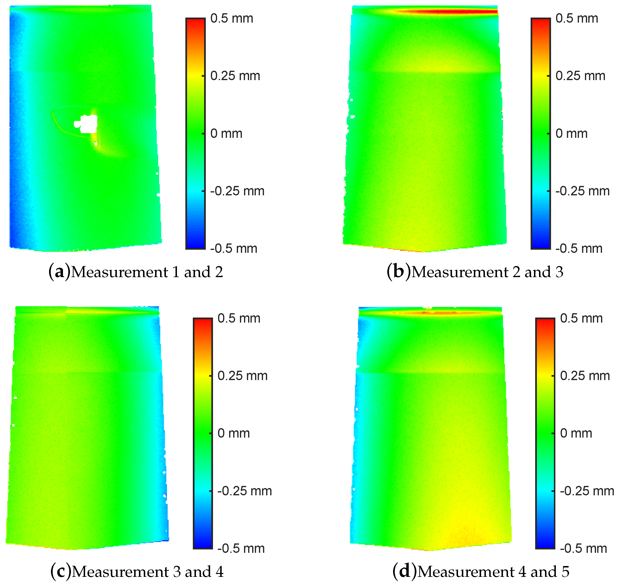
| 1, 2 | 344 | 82 | −0.457 | 0.333 | 0.105 |
| 2, 3 | 194 | 23 | −0.549 | 0.701 | 0.096 |
| 3, 4 | 152 | 26 | −0.599 | 0.417 | 0.139 |
| 4, 5 | 234 | 25 | −0.451 | 0.457 | 0.142 |
© 2016 by the authors; licensee MDPI, Basel, Switzerland. This article is an open access article distributed under the terms and conditions of the Creative Commons by Attribution (CC-BY) license (http://creativecommons.org/licenses/by/4.0/).
Share and Cite
Von Enzberg, S.; Al-Hamadi, A.; Ghoneim, A. Registration of Feature-Poor 3D Measurements from Fringe Projection. Sensors 2016, 16, 283. https://doi.org/10.3390/s16030283
Von Enzberg S, Al-Hamadi A, Ghoneim A. Registration of Feature-Poor 3D Measurements from Fringe Projection. Sensors. 2016; 16(3):283. https://doi.org/10.3390/s16030283
Chicago/Turabian StyleVon Enzberg, Sebastian, Ayoub Al-Hamadi, and Ahmed Ghoneim. 2016. "Registration of Feature-Poor 3D Measurements from Fringe Projection" Sensors 16, no. 3: 283. https://doi.org/10.3390/s16030283
APA StyleVon Enzberg, S., Al-Hamadi, A., & Ghoneim, A. (2016). Registration of Feature-Poor 3D Measurements from Fringe Projection. Sensors, 16(3), 283. https://doi.org/10.3390/s16030283