
A Novel Method of Multi-Information Acquisition for Electromagnetic Flow Meters

Abstract
:1. Introduction
2. Detecting Mechanism
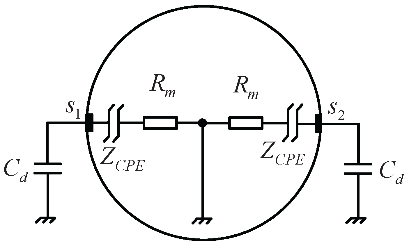
2.1. Model of the Transducer


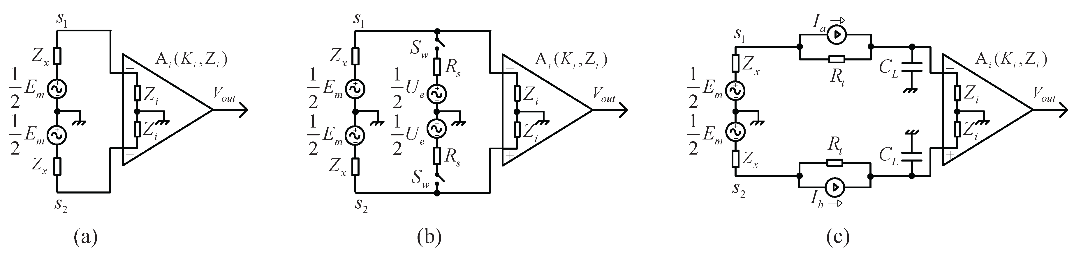
2.2. Fluid-Velocity Signal Loss under Different Modes of Electrical Excitation

| 0.1 | 0.99% | 0.33% | 0.1% |
| 1 | 9.08% | 3.22% | 0.99% |
| 10 | 49.75% | 24.81% | 9% |
| (ms) | |||
|---|---|---|---|
| = 1 nF | = 10 nF | = 100 nF | |
| 0.1 | 0.52 | 5.2 | 52 |
| 1 | 5 | 50 | 500 |
| 10 | 50 | 500 | 5000 |
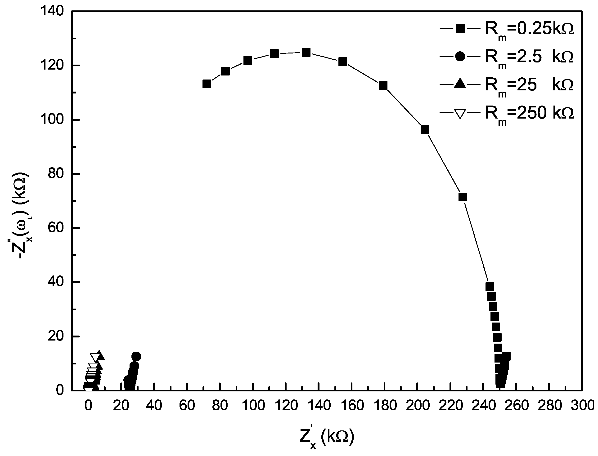
2.3. EIS Measurement Principle in Serial Electrical Excitation Mode
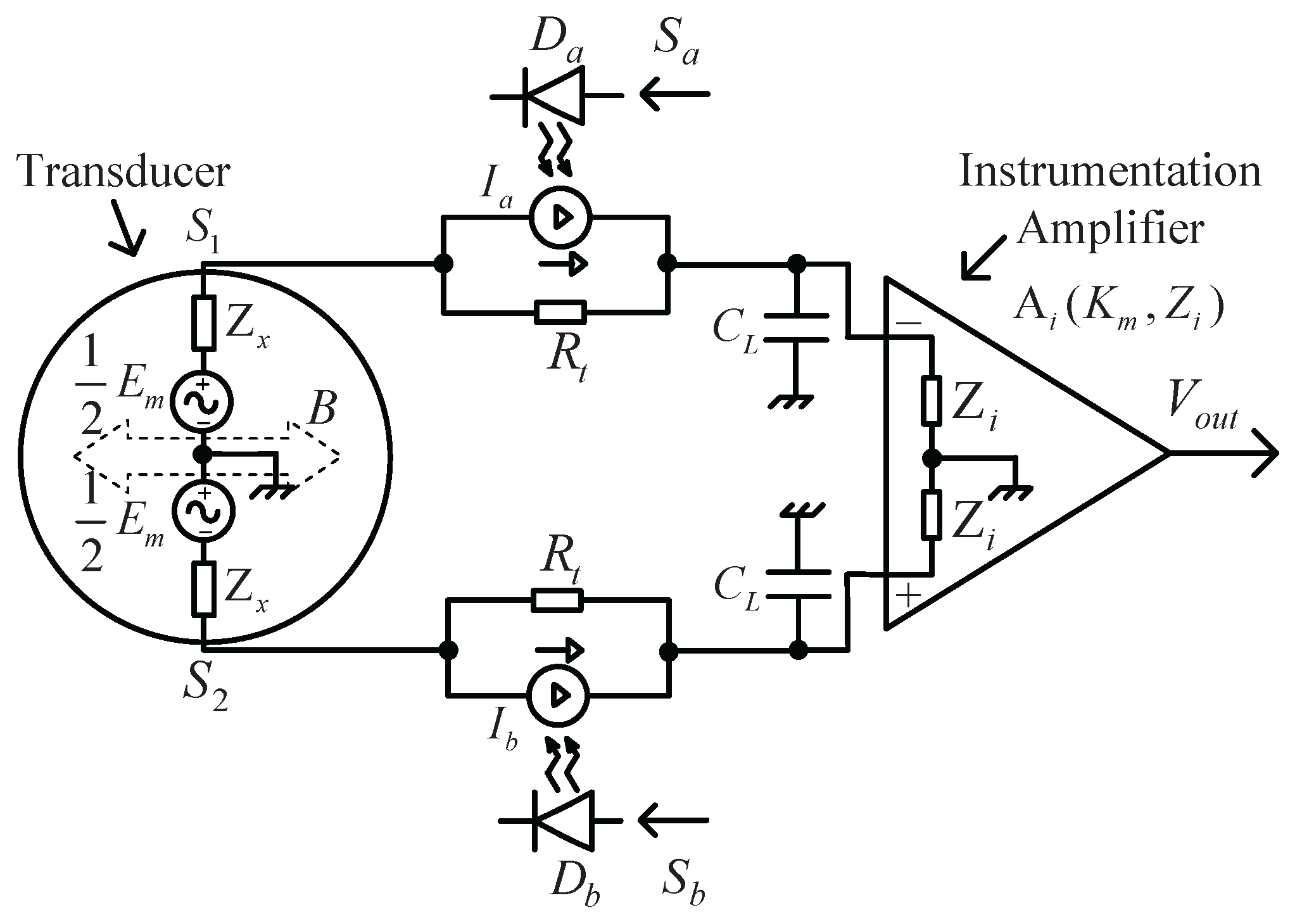
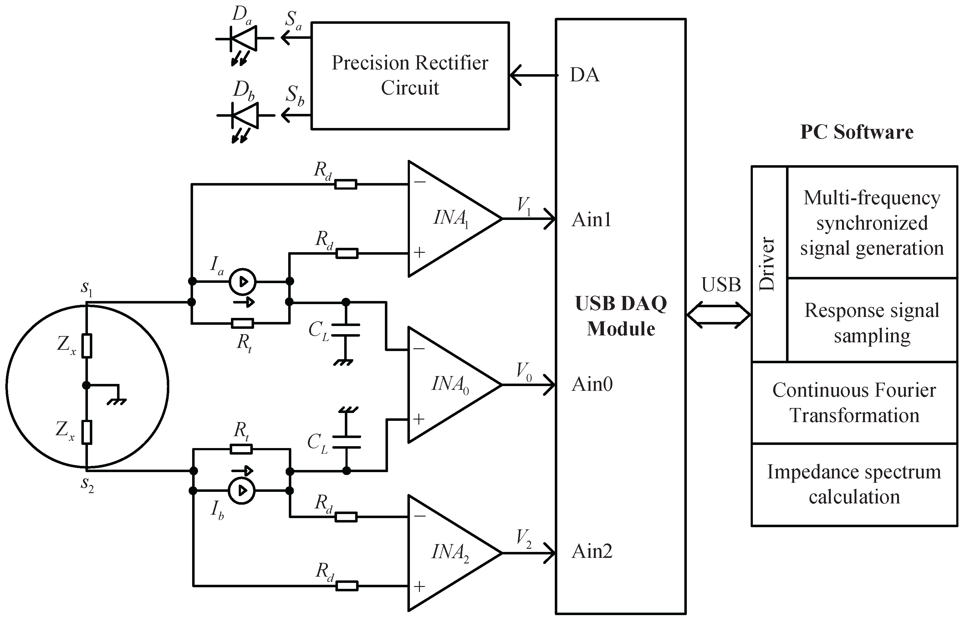
3. System Realization
4. Experimental Results and Discussion
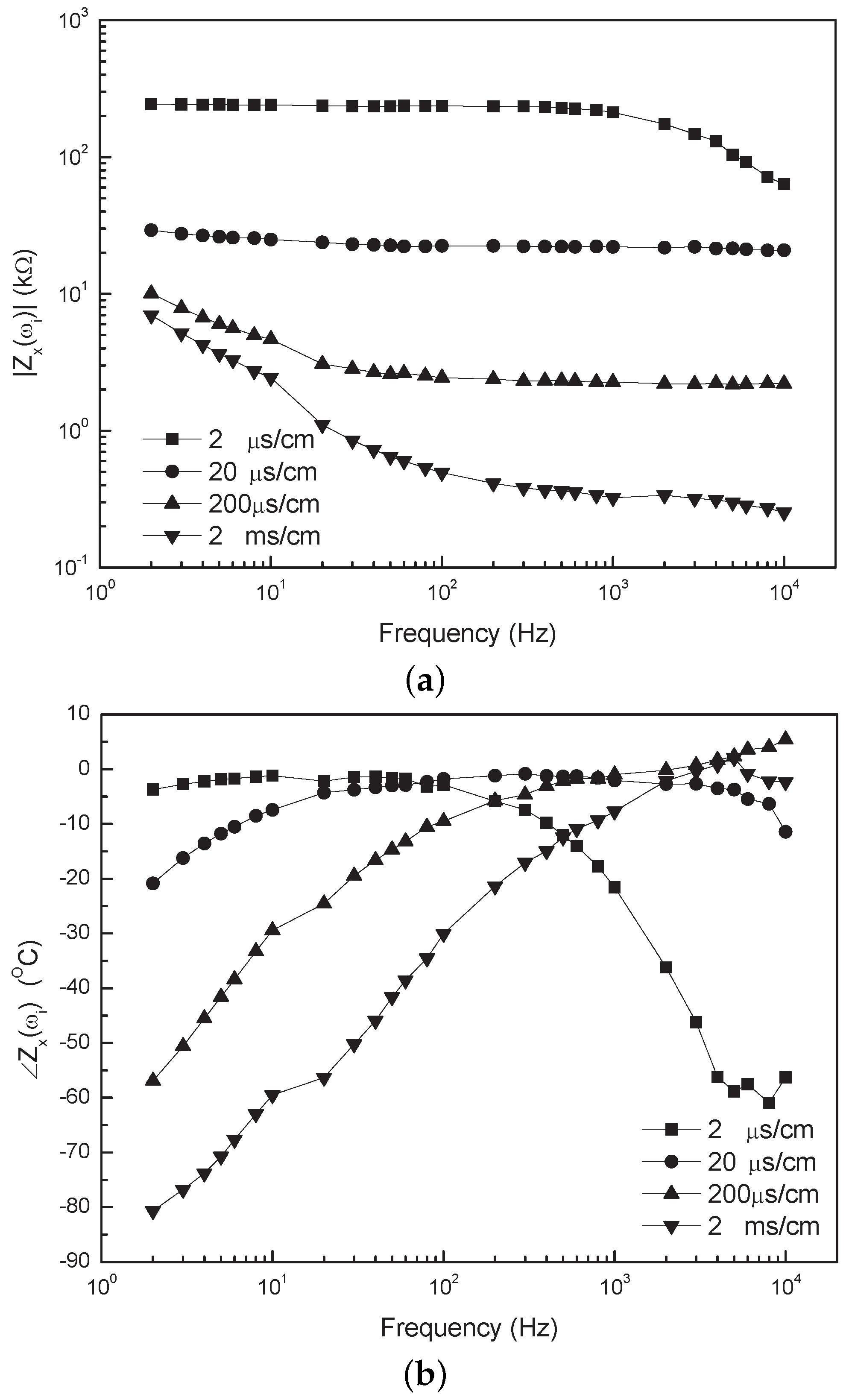
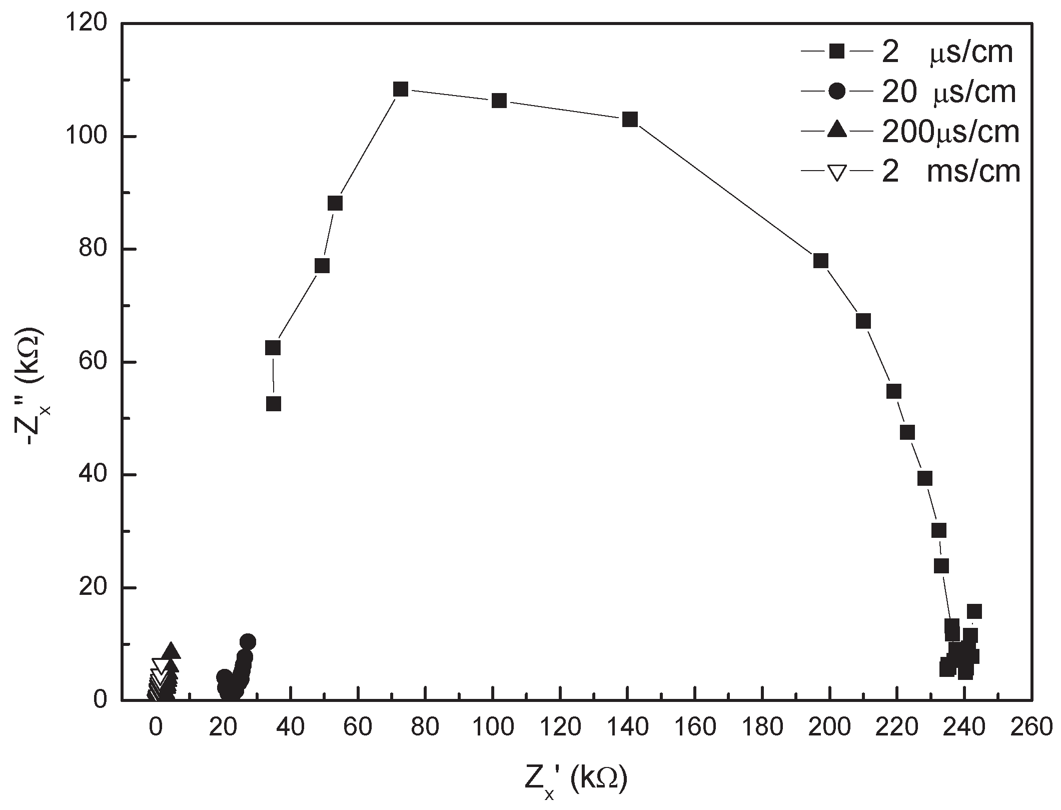
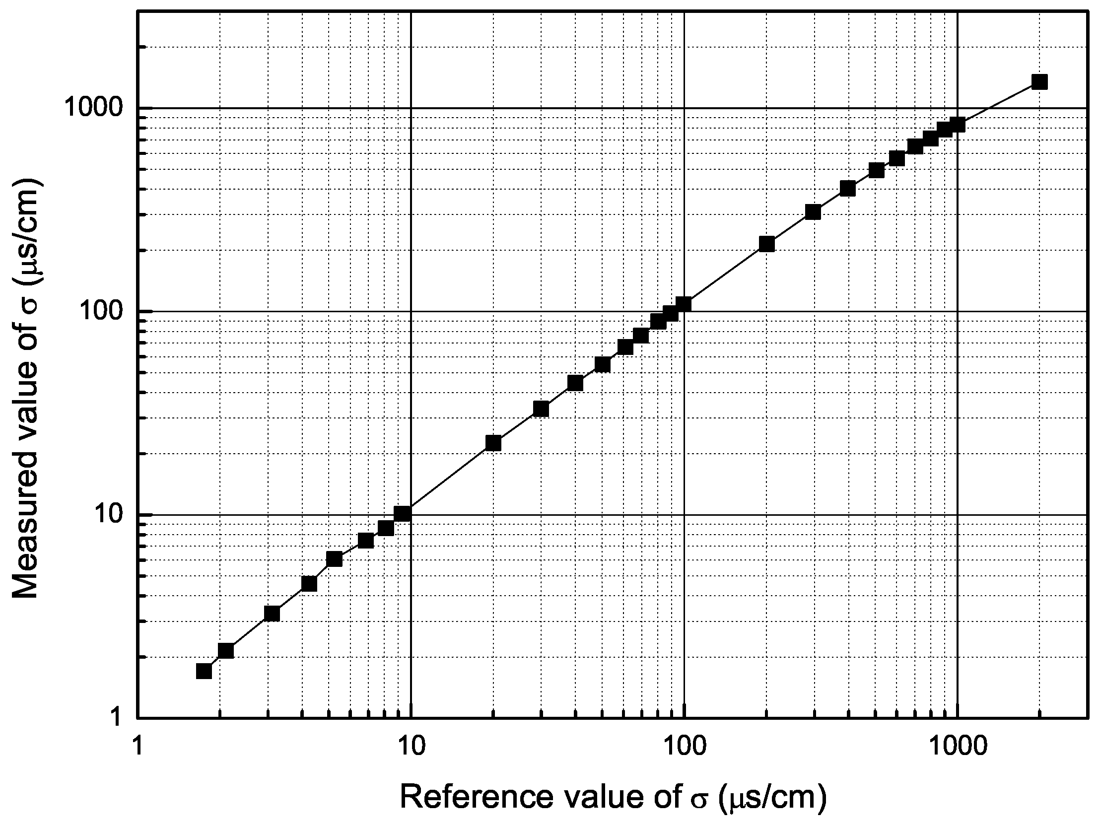
4.1. Medium Conductivity Identification
4.2. Electrode Adhesion Detection
| Conditions | Q | n | ||
|---|---|---|---|---|
| k | ||||
| Case 1 | 200 μS/cm | 2.4 | 14.7 | 0.8 |
| 400 μS/cm | 1.24 | 15.7 | 0.81 | |
| 600 μS/cm | 0.85 | 16 | 0.81 | |
| 1 mS/cm | 0.5 | 16.7 | 0.75 | |
| tap water | 1.518 | 15 | 0.78 | |
| Case 2 | soft cream | 0.946 | 26 | 0.86 |
| hard cream | 2.57 | 21 | 0.8 | |
| chewing gum | 18 | 12 | 0.63 | |
| MoS2 | 0.007 | 5 | 0.23 | |
5. Conclusions
Acknowledgments
Author Contributions
Conflicts of Interest
References
- Schrag, D.; Hencken, K.; Andenna, A. From Flowmeter to Advanced Process Analyser. In Proceedings of the International Conference on SENSOR + TEST’11, Nurnberg, Germany, 6–9 June 2011; pp. 67–72.
- Aisopou, A.; Stoianov, I.; Graham, N.J.D. In-pipe water quality monitoring in water supply systems under steady and unsteady state flow conditions: A quantitative assessment. Water Res. 2012, 46, 235–246. [Google Scholar] [CrossRef] [PubMed]
- Lambrou, T.P.; Anastasiou, C.C.; Panayiotou, C.G.; Polycarpou, M.M. A low-cost sensor network for real-time monitoring and contamination detection in drinking water distribution systems. IEEE Sens. J. 2014, 14, 2765–2772. [Google Scholar] [CrossRef]
- Hencken, K.; Schrag, D.; Grothey, H. Statistical Signal Processing for the Detection of Gas Bubbles in a Magnetic Flowmeter. In Proceedings of the IEEE Sensors, Lecce, Italy, 26–29 October 2008; pp. 1410–1413.
- Hencken, K.; Schrag, D.; Grothey, H. Impedance spectroscopy for diagnostics of magnetic flowmeter. In Proceedings of the IEEE Sensors, Lecce, Italy, 26–29 October 2008; pp. 1112–1115.
- Cao, J.L.; Li, B. Study on methods of empty pipe detection for electromagnetic flowmeter. Chin. J. Sci. Instrum. 2006, 27, 643–647. [Google Scholar]
- Maalouf, A.I. A validated model for the electromagnetic flowmeter’s measuring cell: Case of having an electrolytic conductor flowing through. IEEE Sens. J. 2006, 6, 623–630. [Google Scholar] [CrossRef]
- Ishikawa, I.; Oota, H. Electromagnetic Flowmeter. U.S. Patent 6,804,613, 12 October 2004. [Google Scholar]
- Schrag, D.; Grothey, H.; Hencken, K.; Naegele, M. Method and Device for Operating a Flow Meter. U.S. Patent 7,546,212, 9 June 2009. [Google Scholar]
- Rufer, H.; Drahm, W.; Schmalzried, F. Method for Predictive Maintenance and/or Method for Determining Electrical Conductivity in a Magneto-inductive flow-Measuring Device. U.S. Patent 8,046,194, 25 October 2011. [Google Scholar]
- Cao, J.L. Study on Muti-parameter Measurement Electromagnetic Flowmeter and its Realization Techniques. Ph.D. Thesis, Shanghai University, Shanghai, China, 2007. [Google Scholar]
- Shen, T.F.; Li, B.; Cao, J.L. Parallel Type Electromagnetic Flowmeter with Dual Excitations. CN Patent 100,491,928, 27 May 2009. [Google Scholar]
- Yokogawa Electric Corporation. User’s Manual-AXF Magnetic Flowmeter Integral Flowmeter [Software Edition]. Available online: https://www.yokogawa.com/fld/pdf/AXF/IM01E20C02-01E.pdf (accessed on 23 December 2015).
- Cui, W.H.; Li, B. A new Approach for the Parameter Measurement of Fluid Conductivity in an Electromagnetic Flow Meter. In Proceedings of the 16th International Flow Measurement Conference, Paris, France, 24–26 September 2013; pp. 274–277.
- Kitai, A. Principles of Solar Cells, LEDs and Diodes: The Role of the PN Junction; John Wiley & Sons: Hoboken, NJ, USA, 2011. [Google Scholar]
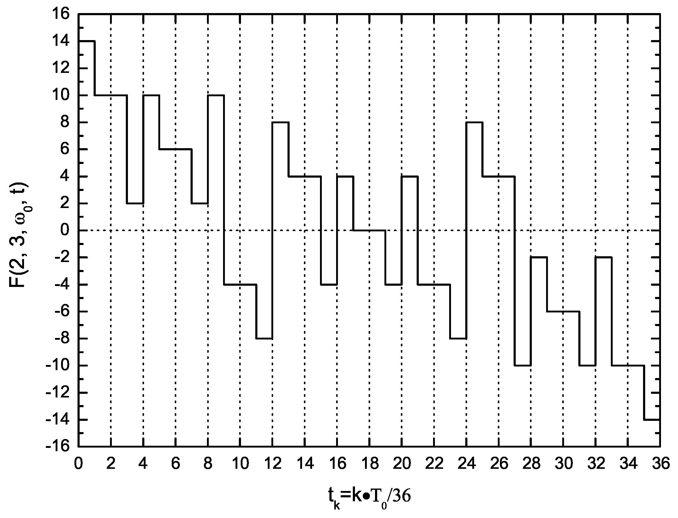
- Cui, W.H.; Li, B.; Li, X.W. A New Synthesis Method of Uniform-amplitude Multi-frequency Synchronous Excitation Signals Based on Dual-base Power Sequences. Math. Probl. Eng. under review.
- Chang, B.Y.; Park, S.M. Electrochemical impedance spectroscopy. Annu. Rev. Anal. Chem. 2010, 3, 207–229. [Google Scholar] [CrossRef] [PubMed]
- Macdonald, J.R.; Barsoukov, E. Impedance Spectroscopy: Theory, Experiment, and Applications; Wiley-Interscience: New York, NY, USA, 2005. [Google Scholar]
- Bard, A.J.; Faulkner, L.R. Electrochemical Methods: Fundamentals and Applications, 2nd ed.; John Wiley & Sons Inc.: Hoboken, NJ, USA, 2001. [Google Scholar]
- Shercliff, J. The Theory of Electromagnetic Flow-Measurement; Cambridge University Press: London, UK, 1962. [Google Scholar]
© 2015 by the authors; licensee MDPI, Basel, Switzerland. This article is an open access article distributed under the terms and conditions of the Creative Commons by Attribution (CC-BY) license (http://creativecommons.org/licenses/by/4.0/).
Share and Cite
Cui, W.; Li, B.; Chen, J.; Li, X. A Novel Method of Multi-Information Acquisition for Electromagnetic Flow Meters. Sensors 2016, 16, 25. https://doi.org/10.3390/s16010025
Cui W, Li B, Chen J, Li X. A Novel Method of Multi-Information Acquisition for Electromagnetic Flow Meters. Sensors. 2016; 16(1):25. https://doi.org/10.3390/s16010025
Chicago/Turabian StyleCui, Wenhua, Bin Li, Jie Chen, and Xinwei Li. 2016. "A Novel Method of Multi-Information Acquisition for Electromagnetic Flow Meters" Sensors 16, no. 1: 25. https://doi.org/10.3390/s16010025
APA StyleCui, W., Li, B., Chen, J., & Li, X. (2016). A Novel Method of Multi-Information Acquisition for Electromagnetic Flow Meters. Sensors, 16(1), 25. https://doi.org/10.3390/s16010025