1. Introduction
Driver fatigue has been identified worldwide as one of the main reasons for traffic accidents. According to the information from NHTSA (National Highway Traffic Safety Administration) of the United States (US), there are about 100,000 crashes caused by driver drowsiness or fatigue annually, and these accidents cause more than 1500 fatalities and 71,000 injuries [
1,
2,
3,
4]. In Europe, driver fatigue causes about 6000 deaths every year [
5] and many studies claim that the main cause of the 15%–20% of all traffic accidents is driver fatigue [
3,
6,
7]. In 2010, the Ministry of Public Security of the People’s Republic of China reported about 4,000,000 traffic accidents, and the number is still increasing. Mental fatigue accidents do not only exist in ordinary road traffic, but also in airline and railway industries. In these industries, a great part of accidents is due to drivers’ wrong operations caused by fatigue. In 1996, Morris and Miller did an experiment using a flight simulator, and found that pilots would fall into a drowsy status after about four and a half hours, then the possibility they would undertake incorrect operations would significantly increase [
8]. Compared with the normal civil field, accidents in these industries would cause much worse outcomes, even a disaster. It would be very helpful to detect drivers’ fatigue levels and provide an alert before it is too late to avoid or at least reduce these accidents.
Driver fatigue is caused by lots of factors, such as stress, long time driving, lack of rest or continuous sleep, and monotonous driving environments [
9,
10,
11], which seriously affect driving performance. It is a very complex mechanism, which is still not fully understood. Driver fatigue is also reflected in many ways, such as increase of a driver’s reaction time, worse vehicle control performance, changes in brain activity, frequency of eye blink/movement, and heart rate. Current related researches could be divided roughly into two classes. The first class is based on a driver’s vehicle control behaviors. For this kind, it is necessary to determine which part of these behavioral changes is caused by driver fatigue and which is caused by traffic conditions and other environmental factors [
5]. The second class is based on driver’s physiological signals, such as changes of chemical components in blood and heart rate, and electrical or magnetic signals from brain activity, which could be collected from blood samples, electrocardiogram (ECG), electroencephalogram (EEG) and magnetoencephalography (MEG), respectively [
1]. Since methods to collect chemical signals are usually intrusive and equipment to collect magnetic signals is usually huge and expensive, the EEG signal offers high temporal-resolution and the procedure to collect it is quite fast and non-intrusive. As the EEG equipment is cheap and portable, it has been widely used to study many mental and driver fatigue states in real environments, and numerous results reported [
4,
5,
12,
13,
14,
15] showed how the EEG may be one of the most predictive and reliable physiological indicators [
16,
17].
In the latest 20 years, many researchers have started to study the human brain in terms of interactions among the different brain areas [
18,
19]. In particular, in the last few years, some researchers have proposed the concept of the
Brain Network. In a brain network, regions of the human brain (or EEG channels) are treated as
Nodes, while the link between two nodes are called
Edges. By the Graph Theory, specific indices are defined to calculate and quantify the connectivity strength between each pair of nodes. Threshold procedures are used with the aim of eliminating spurious connections due to the presence of no-physiological signals (noise). The nodes and the relative edges form network structures, which are called
Brain Networks. There are two kinds of connectivity that are possible to estimate:
Functional Connectivity and
Effective Connectivity [
20,
21]. These networks are called
brain functional networks and
brain effective networks, respectively. Functional connectivity is a statistical measure of the temporal correlations between spatially separated neurophysiologic events (
undirected relationship). Generally, the indexes used to quantify the functional connectivity are the Pearson correlation, partial correlation, partial coherence, mutual information and synchronization likelihood. The effective connectivity is instead a measure of causal influence from one neural unit to another (
directed relationship) and it is normally estimated by Granger causality model, dynamic causality model and structural equation model. In the presented study, the brain effective networks, based on spectral Granger causality (GC), have been used to study driver fatigue. Driving accidents caused by fatigue are directly induced by long reaction time, lethargy or other symptoms. It has been reported that consciousness depends on the brain’s ability to integrate information [
22,
23] and integration is usually better understood with effective connectivity [
21]. For example, during non-rapid eye movement sleep, one possible reason for losing consciousness is the breakdown of cortical effective connectivity [
24]. Current EEG-based methods to study fatigue detection could not describe the interactions between different brain regions and measure the brain’s ability to integrate information. The Granger-Geweke causality is able to measure the strength of effective connectivity and it has been widely applied to investigate the dynamic relationship between different brain regions [
25,
26]. The basic idea has been first proposed by Wiener [
27], it was successively formalized by Granger using autoregressive model and then Geweke proposed the first spectral decomposition of Granger’s time-domain causality [
28,
29,
30]. Since EEG data contains many different frequency components, Granger-Geweke model has been chosen here to calculate the causality strength of connectivity estimated from the gathered EEG data. In order to figure out the feasibility of using spectral Granger causality to investigate the driver fatigue, and to reduce the complexity of the analysis, only pair-wise spectral Granger causality has been considered in this work.
This study has two main goals: (1) try to find out the differences in terms of EEG pattern between the alert status, at the beginning of a long time driving and the pattern of the drowsy status at the end of the driving experiment by using brain effective network method. These differences could be used as indicators for fatigue detection; (2) try to find out which part of human brain cortex most likely relate to driver fatigue, which could be used to decide the most appropriated EEG electrodes position scheme in successive experiments. The paper is organized as follow.
Section 2 introduces the experiment design, the EEG data recording procedure, and the methodology for the estimation of the brain network properties and describes the analysis procedure.
Section 3 presents the results and
Section 4 the meanings of the obtained results are discussed.
Section 5 provides the conclusions for the work developed.
2. Material and Methods
2.1. Experiment Design
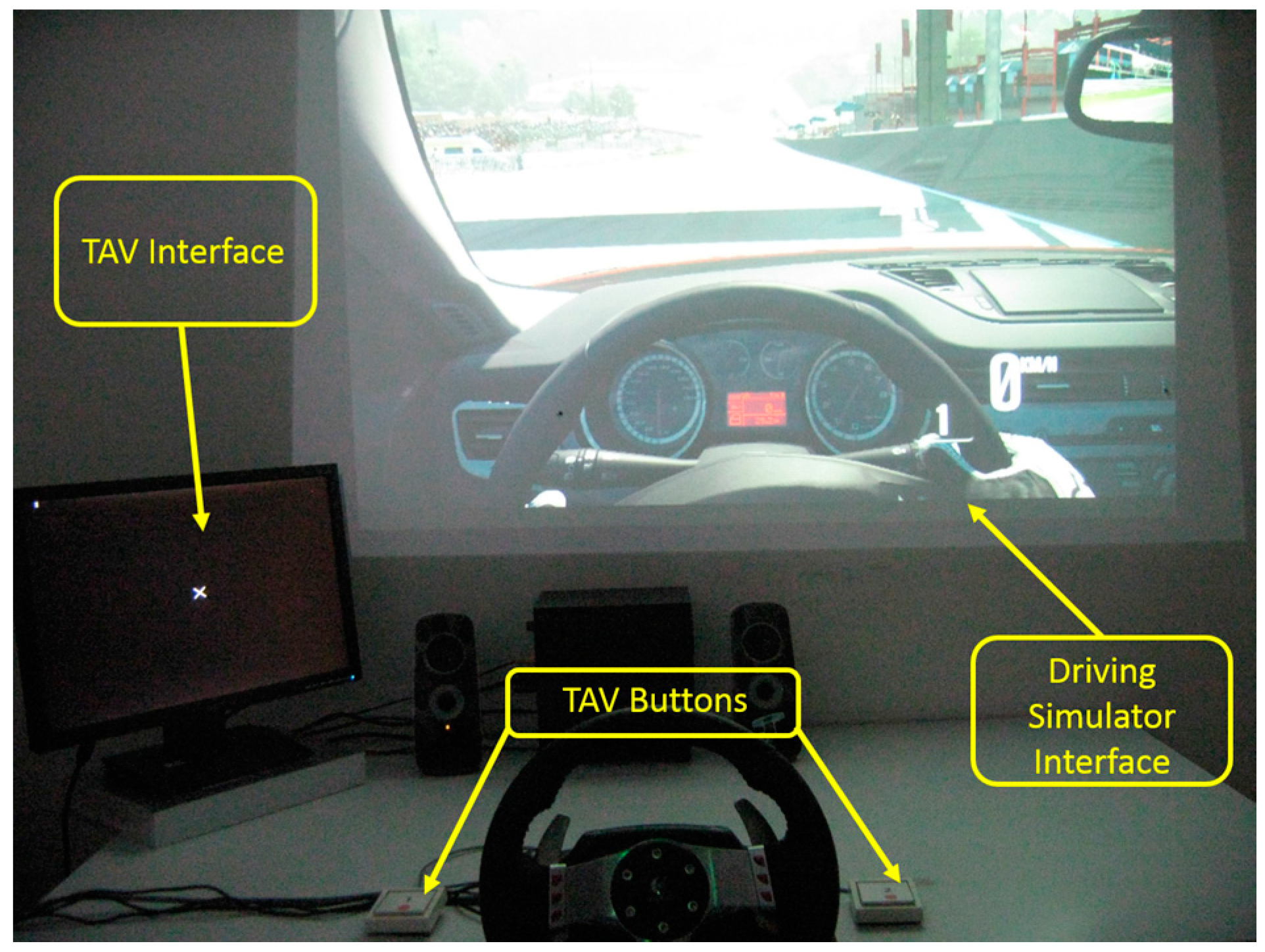
A driving simulation experiment has been designed to make the subjects drowsy quickly. In the experiment, a commercial software named
Need for Speed-Shift 2 Unleashed (NFS-S2U) has been used to simulate the driving environment, since it could provide a quite real visual effect (
Figure 1).
Figure 1.
Experimental setup. Note at the bottom of the figure the wheeldrive and beside it the two TAV buttons needed for the execution of the additional tasks other than simple drive (see text for explanations).
Figure 1.
Experimental setup. Note at the bottom of the figure the wheeldrive and beside it the two TAV buttons needed for the execution of the additional tasks other than simple drive (see text for explanations).
In order to achieve the aims of the study, the driving simulation scene was set to the night condition, which was consistent with the real experiment time. In fact, all the experiments were performed between 6 p.m. and 9 p.m., because people are more likely to become tired during this time after daytime work. The selected car was the
Alfa Romeo—Giulietta QV (1750TBi, 4 cylinders, 235 HP) and the experimental circuit chosen was the Spa–Francorchamps route (Belgium). The experimental protocol included EEG baseline recordings (Eyes Opened—OA; Eyes Closed—OC) and eight driving conditions (
WUP,
PERF,
TAV3,
TAV1,
TAV5,
TAV2,
TAV4 and
DROWSY). For each condition, subjects were asked to drive two laps of the circuit along the selected track. In the
WUP (Warm-Up) condition, subjects drove without any requirements, while in the
PERF (Performance) condition, subjects were asked to reduce the total time by 2% of the previous total time without committing mistakes (e.g., off-road driving). In the
TAVx conditions, the subjects had to keep track of the total time taken in the PERFO conditions and, at the same time, to execute the
Task of Alert and Vigilance—TAV (see
Section 2.2 for more details). The different levels of the TAV have been used to modulate the difficulty of the global task, and it consists of an alert visual stimulus and a vigilance acoustic stimulus. The difference among the five
TAV’s levels consisted in the stimulus rate, which is represented by the number
x, from 1 (EASY) to 5 (HARD). The sequence of
TAVx conditions was proposed randomly to the subjects to avoid any expectation and habituation effects. In the last experimental condition (
DROWSY), subjects were asked to drive as in urban centers, that is around a speed limit of 50 km/h. Such monotonous driving conditions were used to induce the drowsy state. After each condition, subjects had to fill out the
NASA-Task Load Index (NASA-TLX) and the
Karolinska Sleepiness Scale (KSS) form to collect subjective evaluations of the task workload and driver’s sleepiness [
31].
2.2. Task of Alert and Vigilance
The Task of Alert and Vigilance (TAV) was the second task to pay attention at while the subject was performing the driving simulation in the TAV
x (
x ranges from 1 to 5) conditions. The
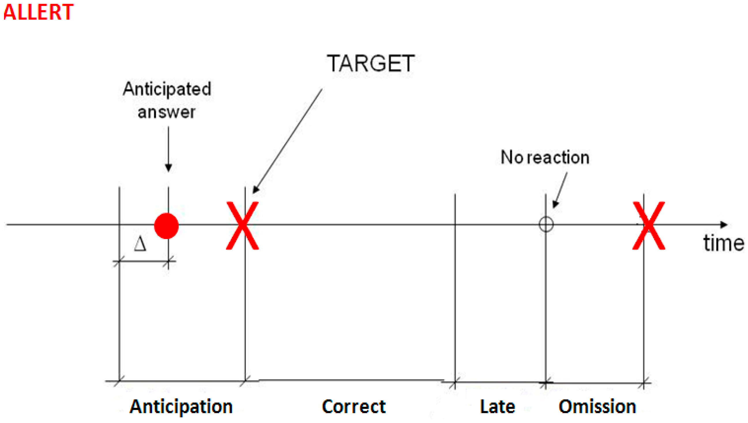
Alert task (
Figure 2) consisted in pressing a button every time an “X” was shown on the screen. It was used to simulate possible obstacles and other cars on real roads. Since the target was presented in the center of the screen, placed 70 (cm) from the user, the subject had 1500 (ms) for pressing the correct button (button number 2) as soon as possible, and the possible reaction times should be “Anticipation”, “Correct”, “Late” and “Omission”.
Figure 2.
Alert task: The TARGET is the stimulus shown on the screen and the subject has to answer to it as soon as possible. The possible reaction times could be: early, correctly, late or no answer.
Figure 2.
Alert task: The TARGET is the stimulus shown on the screen and the subject has to answer to it as soon as possible. The possible reaction times could be: early, correctly, late or no answer.
Anticipation means that the subject pressed the button before the presentation of the stimulus plus a ∆ time estimated around 350–500 ms.
Correct corresponds to a reaction in the time interval from the presentation of the “X” to 1500 ms after it, otherwise the answer was classified as
Late and, if the reaction time exceed 2000 ms, it was classified as
Omission. In case of “not correct answer”, in the log performance file there was a −1, −2 or −3, respectively, or 0 in case of “correct answer”. In
Figure 2, the time definitions of the different answers are shown. At the same time, the subjects had to face the
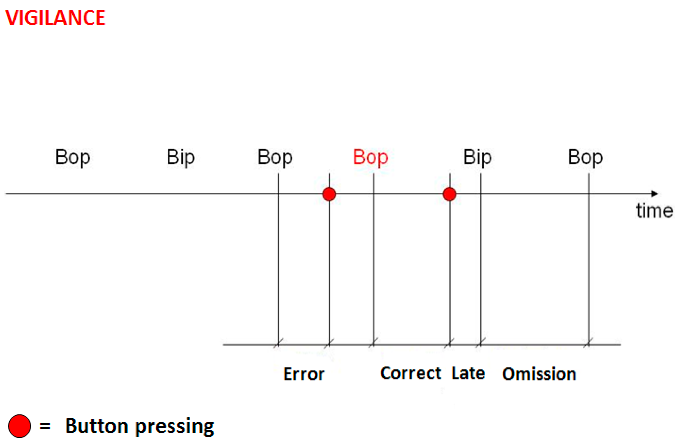
Vigilance task (
Figure 3) which was the identification of the same acoustical frequency of consecutive acoustic tones (low and high frequency) by pressing the corresponding button (button number 1) before the next tone impulse, with an inter-stimulus time of 2000 (ms). A response after this time interval was named as
Late, while
Omission was recorded if there were no answers and
Error if the response did not coincide with the tone impulses. In
Figure 3 is shown an example of a tone sequence and the different types of errors of reaction time. Therefore, one of the tones was used to simulate traffic horns, phone rings, or other occasional sounds which drivers needed to respond to.
Figure 3.
Vigilance task: The target is the identification of the same acoustic tone during the sound sequence, and only after the second identical tone does the subject have to answer by pressing the correct button. If the response is not appropriate, different kinds of errors are provided: early, late, or no answer.
2.3. EEG Signal Recording
During the entire experiment, scalp EEG signals were recorded by using a 16-channels digital system (g.tech USBamp). Fifteen electrodes were placed on the brain according to the 10–20 international system, including Fz, Pz, Oz, Fp1, Fp2, F7, F3, F4, F8, C3, C4, P7, P3, P4, P8. The 16th electrode, placed on the subject’s chest, was used to collect the ECG signal. The ear-lobes were used as reference channels, while the left mastoid as ground channel. The neuro-physiological signals were gathered by a sample rate 256 (Hz). The impedances of the electrodes were kept below 5 kΩ. After each experiment, the recorded signals were checked and EEG data of three subjects were eliminated because of the artifacts. EEG dataset of the WUP and of the DROWSY conditions were selected in line with the aims of the study.
2.4. Experimental Subjects
Twelve volunteers students, aged from 23 to 25 (Mean = 23.7; standard deviation = 0.78), right-handed, with regular driving license and no history of neurological diseases, have taken part in the experiment. They had been told to not consume alcohol, tea, coffee or medicine before the experiment. All the subjects were well trained in order to familiarize them with the driving task and the related software interface.
2.5. EEG Data Preprocessing and Analysis
In order to improve the signal-to-noise ratio and to remove artifacts (e.g., network frequency interference, muscular artifacts,
etc.), a preprocessing procedure was applied to the raw EEG data by using the NPX Lab [
32] software and some
ad-hoc Matlab scripts. Raw scalp EEG data were band-filtered within 1–40 Hz and then the
Independent Component Analysis (ICA) was used to remove the eye-blinks artefacts.
Then, the EEG dataset of each experimental condition was divided into 1 s epochs. The Kwiatkowski-Phillips-Schmidt and Shin (KPSS) test was run for each epoch to check if the data was stationary [
33]. Stationary EEG data were used to calculate pair-wise spectral Granger Causality (GC) values in delta band (1–4 Hz), theta band (4–8 Hz), alpha band (8–13 Hz) and beta band (13–30 Hz), for each EEG channel.
The GC values of each epoch were saved into asymmetric matrices. Then, a threshold procedure was applied to the original GC matrixes to eliminate the spurious connections which were likely caused by no-physiological signals that still remained after the preprocessing.
There are, at least, two methods to set the threshold value: One way is by defining a fixed causality strength, the second one is defining a fixed edge percentage, which is also called
Sparsity. The last method is defined as the ratio between the number of existing edges and the maximum edge number that the brain networks could have. As the GC values are quite different among subjects by the first threshold selection method, it would be quite hard to set a proper threshold value or decide one rule to set different values for all of them. For this reason, the second method has been widely used to explore small-world topology of brain networks [
34,
35,
36] and the edge percentages normally used are 15%–25%, 12.2%–26.7% and 11%–25%. In this study, we have chosen the range of edge percentage (
EdgeP) from 0.05 to 0.6, with a step of 0.05, which is enough to cover the significant small-world property range [
35,
37].
Two Matlab toolboxes, Granger Causal Connectivity Analysis (GCCA) and Brain Smart (BSMART), were used to estimate the Granger causality [
38,
39]. The Brain Connectivity Toolbox (BCT) toolbox was then used to calculate the network properties [
40]. See the Appendix for the details on how the Granger Causality was estimated from EEG data.
2.6. GC Network Analysis
After the threshold procedure, an N × N (N is number of the nodes in the brain network, N = 15 in this paper) directed weighted network could be constructed from one GC matrix. Each node of represents an EEG channel and every directed edge represents an effective connection between two EEG channels. Properties of the GC matrix were calculated according to the formulas described in the following, where V represents the set of all the nodes of the network .
2.6.1. Weighted Degree
In a binary network, the degree of a node describes how many edges are connected to such node, or how many neighbors the node has. For the
i-th node (node
i) of a binary directed brain network, its out-degree tells how many edges of the brain network start from node
i to other nodes, and its in-degree tells how many edges of the network start from other nodes to the node
i [
40]. For weighted brain networks, weighted degree represents the sum of the edges’ strength and the degree of importance of a node; the larger the node’s degree, the more important the node is. Weighted in-degree and out-degree for the
i-th node of a weighted directed network are written as
,
respectively, and the formulas to calculate them are as follow:
In Equations (1) and (2), means strength of the direct effective connectivity from node j to node i, and means from node i to node j.
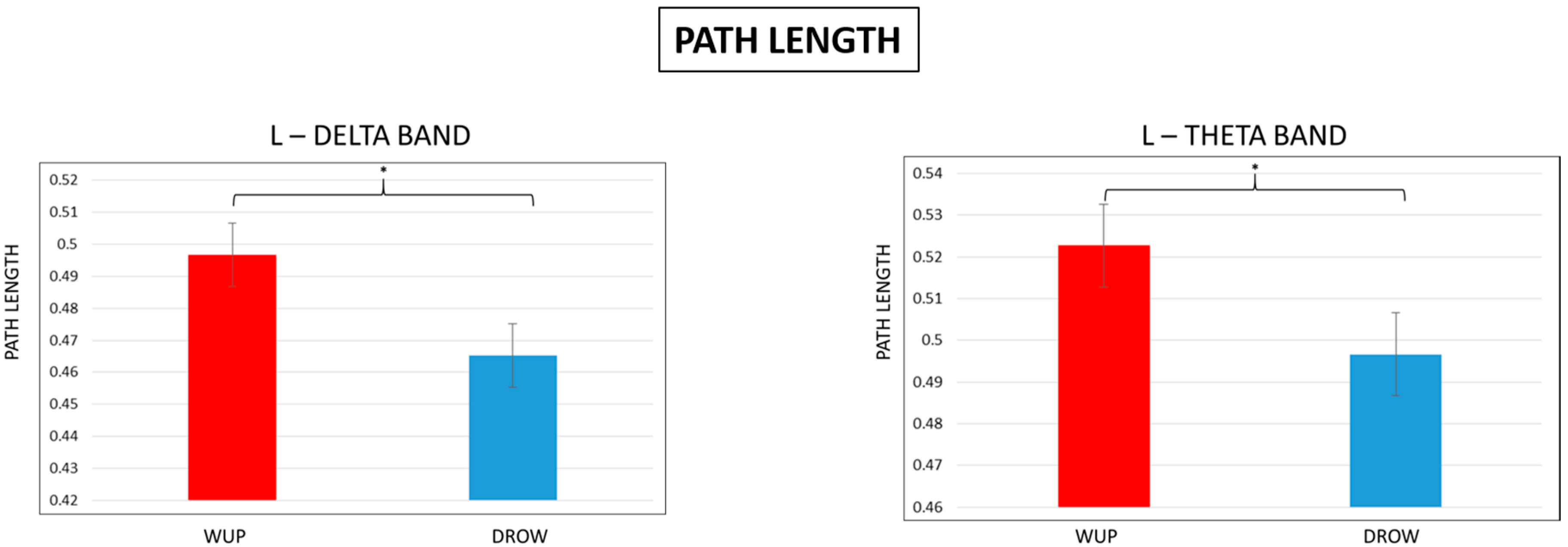
2.6.2. Characteristic Path Length
Characteristic path length (
L) is a global property to measure the typical separation between two nodes [
41], and is one measure of functional integration in brain networks.
L is defined as the average of all the shortest absolute path lengths [
35,
40,
42]. In a weighted GC network
, it means the average strength of the effective connectivity of all the shortest absolute paths. The formula to calculate the L is:
where
is the summarized causality strength of the shortest path between node
i and node
j.
could be binary (by setting all non-zero weighted values to 1) and transformed to a binary network . Based on the procedure, it is easy to know that and are only different at the weight values, besides that they have exactly the same node-set V and the same edge distribution. Characteristic path length of the corresponding binary network provides the average length of all shortest paths between pairs of nodes.
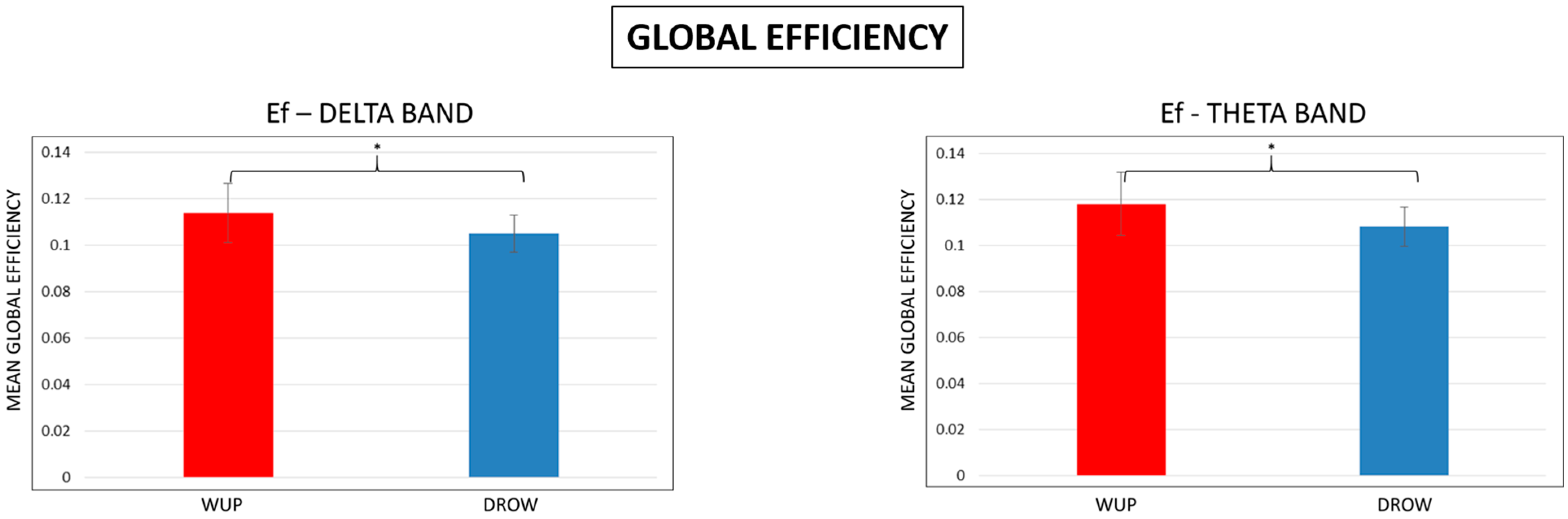
2.6.3. Global Efficiency
Global efficiency (
Eg) of a brain network is defined as the harmonic mean of the inverse of the shortest path length of all pairs of nodes in the network [
40,
43,
44]. It measures the communication efficiency of a network, and is one of the properties which could measure the network’s ability to integrate information [
40]:
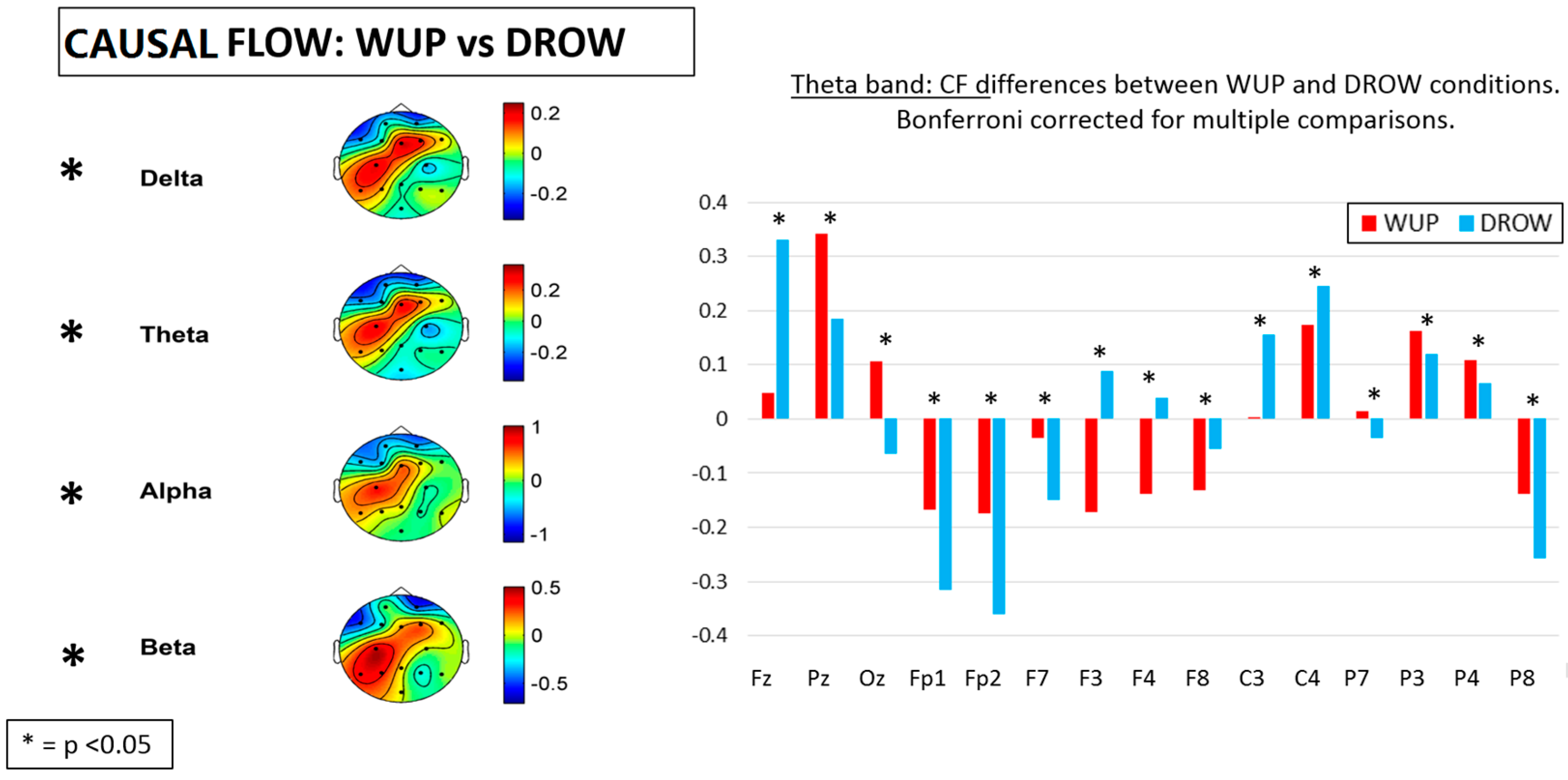
2.6.4. Causal Flow
Causal flow (
CF) of a node is defined as the difference between its out-degree and its in-degree [
38,
45,
46]. For weighted network
,
CF of node
i is calculated as follows:
If a node has a highly positive
CF value, it means granger causal influence from this node to others is much bigger than other nodes to this one. This kind of node is more likely to be the “causal source” of a network. If a node has a quite small negative value, it means this node is largely affected by other nodes. This kind of node is called
Causal Sink of the brain network [
38].
2.6.5. Causal Density
Causal density (
CD) is a novel measure of causal interactivity, which could reflect the overall causal interactivity and the dynamical “complexity” of a system [
46,
47,
48,
49].
CD of a network has been defined as the fraction of interactions between different neuronal elements, electrodes or brain regions that are causally significant. For a weighted network
,
CD of node
i is calculated as:
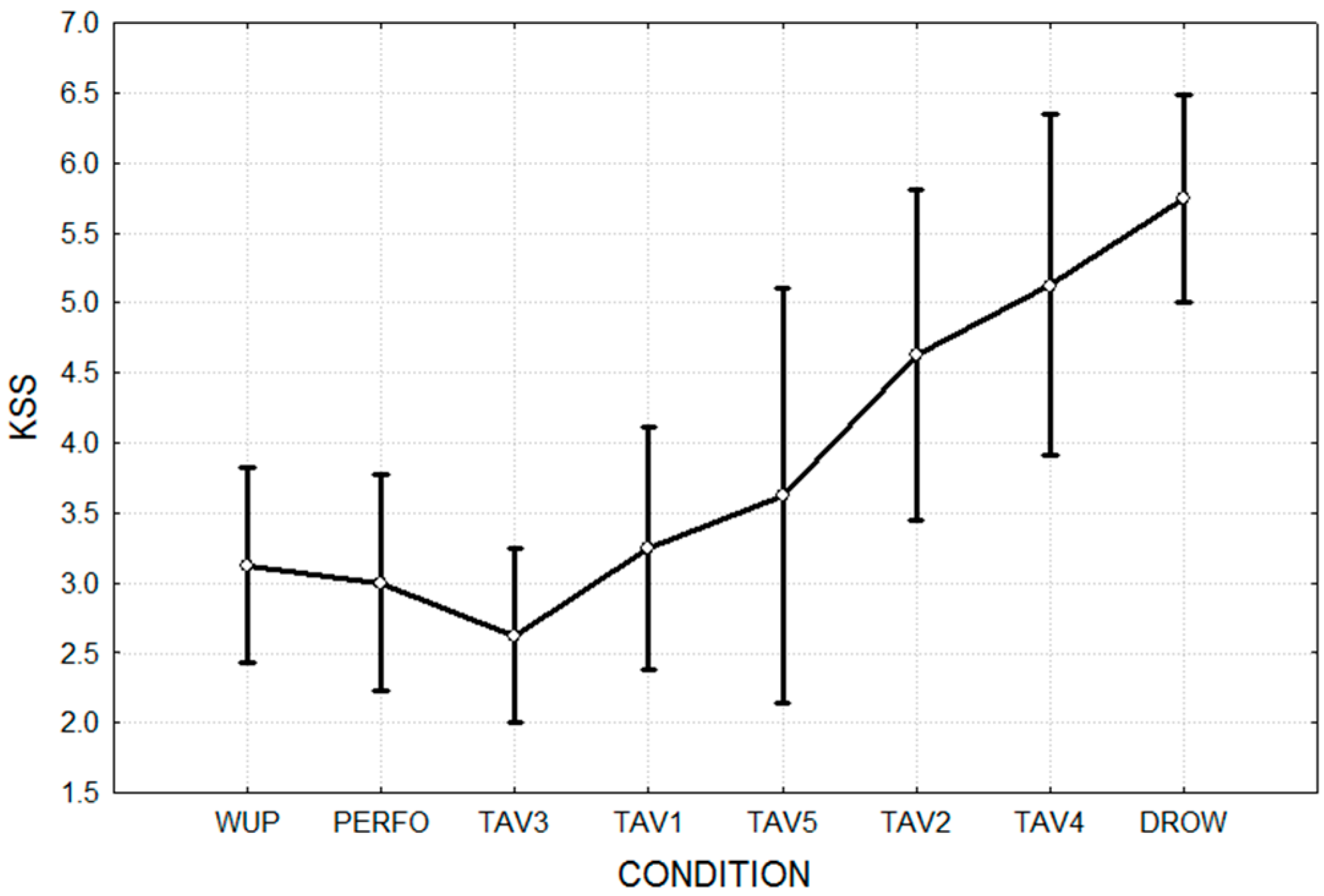
2.7. Statistical Analysis
Repeated measures ANOVA (Confidence Interval, CI = 0.95) and t-tests, with a significant level of α = 0.05, have been used for the statistical validation of the results by using the STATISTICA software (Statsoft). In particular, we have performed two one-way repeated-measures ANOVAs, with the factor CONDITION at eight levels (WUP, PERFO, TAV1 ÷ 5, and DROW), performed separately for the NASA-TLX and the KSS, as independent variables. In addition, we have performed 12 two-tailed paired t-tests to investigate the differences between the WUP and DROW conditions in terms of Granger Causality (GC), Global Efficiency (Eg), Path Length (L), Percentage of Unconnected Nodes (PUN), Casual Flow (CF) and Casual Density (CD). In each test, Bonferroni correction has been used for multiple comparisons to avoid the risk of occurrence of Type I errors.
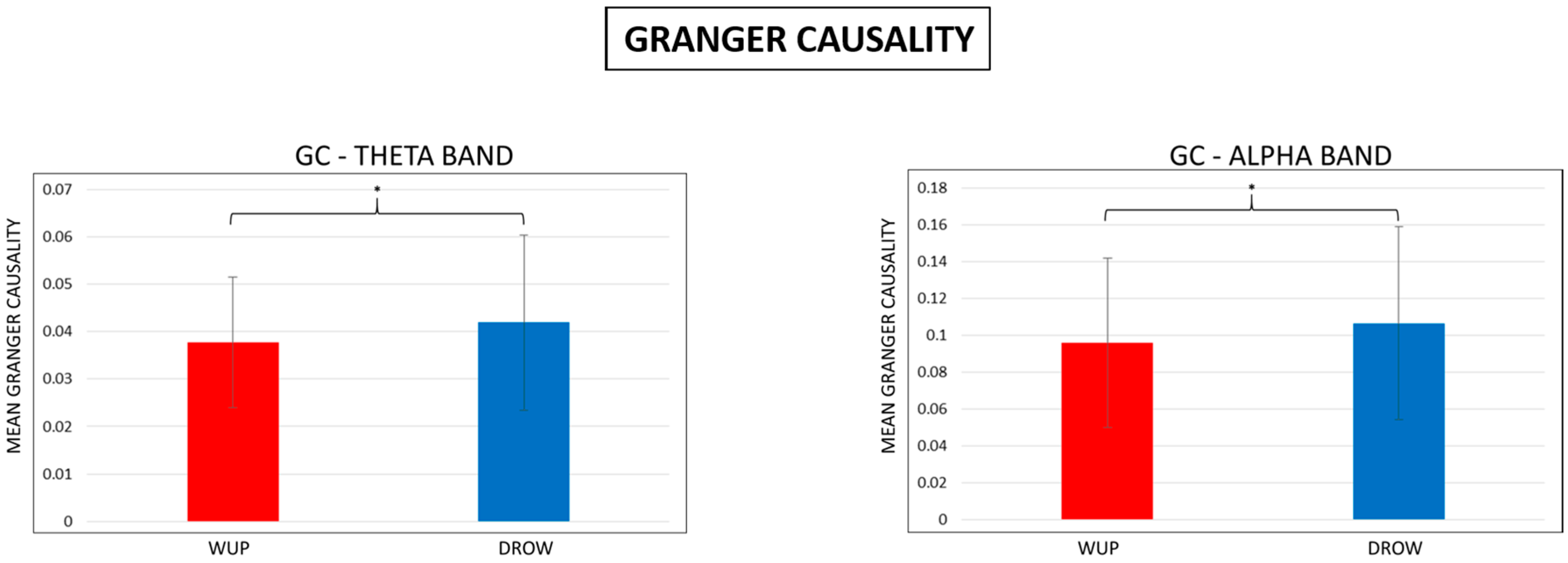
4. Discussion
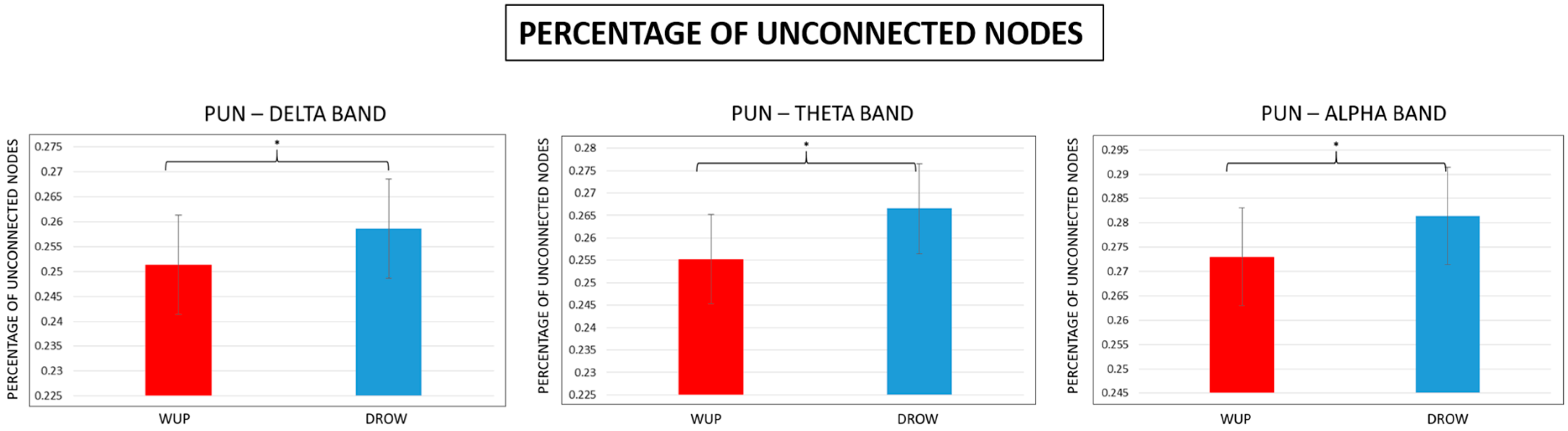
The main results of this study could be summarized as follows: From the WUP to the DROWSY condition, (1) pair-wise Granger causalities (GC) in theta and alpha band increased significantly; (2) in the delta and theta bands, the global efficiency (Eg) and Path Length (L) decreased significantly, and meanwhile the percentage of unconnected nodes increased significantly in delta, theta and alpha bands; (3) CF decreased over the prefrontal, parietal and posterior midline and increased over the frontal and central lobes of the brain cortex in delta, theta, alpha and beta bands, while CD increased almost over the entire brain in the delta, theta and alpha bands.
Pair-wise granger causalities (GC) are the strength of paths between nodes connected directly, their increase meant that these short connections have been enhanced. Global efficiency (Eg) is one measure of brain’s ability to integrate information. Its decrease indicates that the ability has been weakened from WUP to DROWSY condition. The increase of percentage of unconnected nodes meant that there were significant connection breakdowns from WUP to DROW. This indicates that the topology of the brain network changed, which probably made it harder to transmit information between different brain regions. This could be the reason for the global efficiency reduction observed.
The general increment of the CD index over the brain lobes, in particular over the frontal and central lobes, and the simultaneous reduction of CF index over the prefrontal, parietal and posterior midline, from the WUP to DROW conditions indicated that there was much more information converging to the prefrontal lobes when drivers had fallen into a fatigued state. Therefore, these results might indicate that the information processing speed across such brain regions was affected by driver fatigue.
These phenomena were found to be occurring significantly across different frequency bands, such as delta, theta and alpha, especially over the prefrontal, frontal and parietal lobes. It has been reported that the human brain’s attention and memory performance are related with brain activities in the theta and alpha bands, and the brain’s ability to encode information is correlated with activities in the theta band [
50,
51]. Reduced ability to concentrate and react on time is common when drivers become drowsy, and it should be reflected by changes in the brain activities in the theta and alpha bands.


