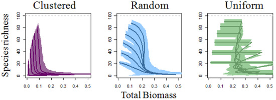
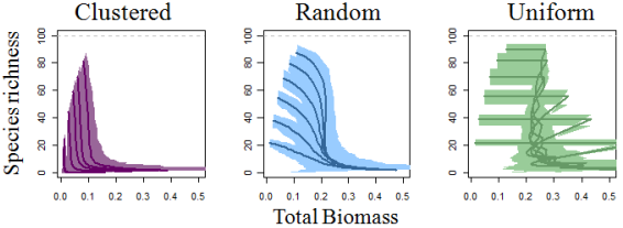
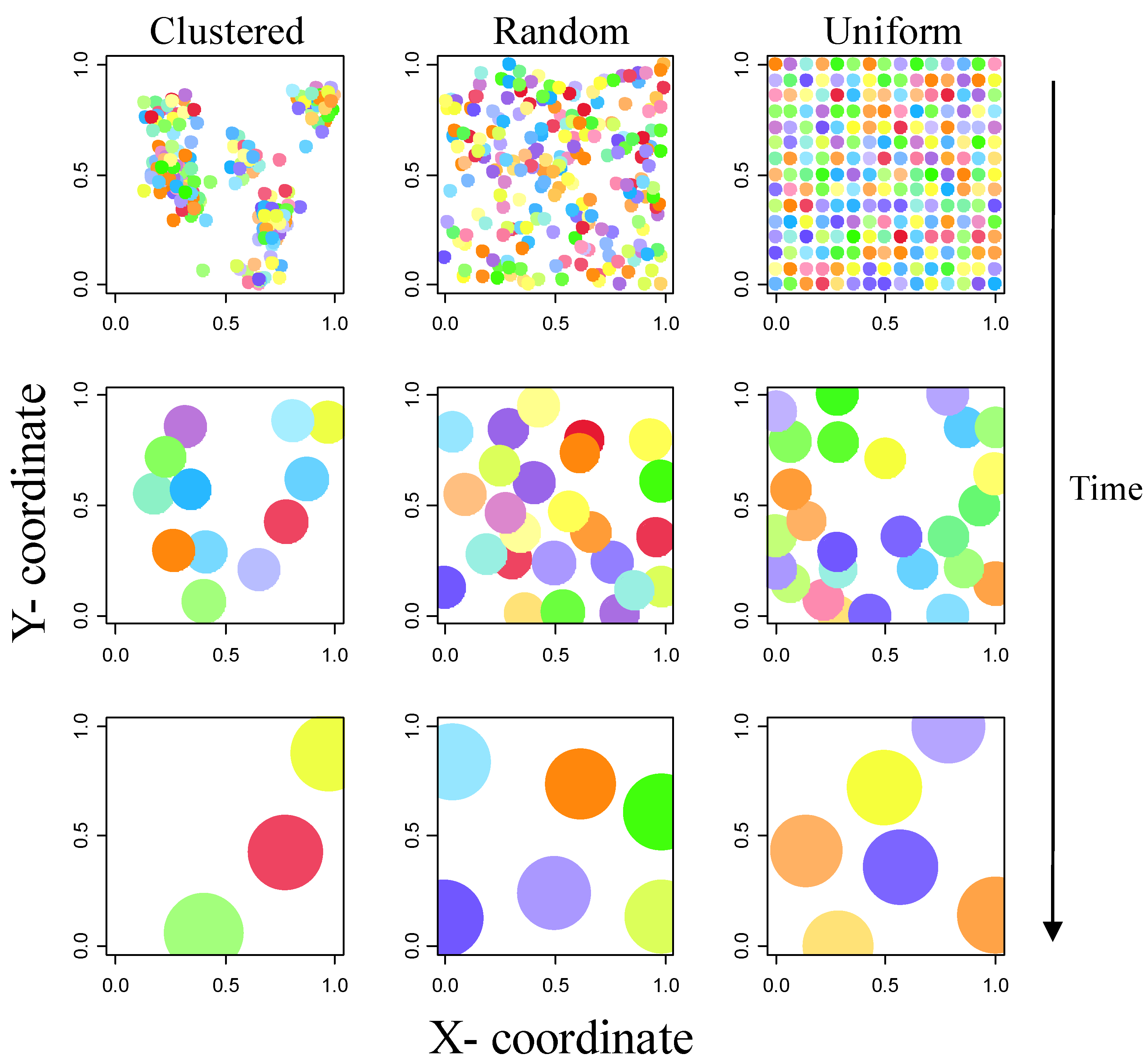
Spatial Structure Alters the Shape of the Unimodal Species Richness-Biomass Relationship in a Neutral Model

Abstract
:
1. Introduction
2. Methods

| Simulation parameter | Value(s) |
|---|---|
| Time | 1–50 |
| Initial diameter | 0.05 |
| Maximum growth rate (ΔDmax) | 0.01 |
| Initial number of individuals | 25, 49, 81, 121, 169, and 225 |
| Relative abundance distribution | uniform |
| Allometric exponent (Biomass α Diameter a) | 8/3 |
| % of individuals that were cluster centers* | 5 |
2.1. Establishment Phase

2.2. Growth Phase
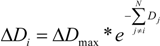
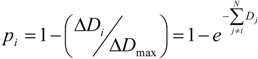
 with
with  in equation 1, where Aij is area of overlap between individual i and its neighbor j. However, this change did not fundamentally alter the patterns, and it increased computation time by a factor of three. Therefore, we only present the results based upon the summed diameters of neighbors.
2.3. Thinning Phase

3. Results
4. Discussion
4.1. Self-thinning and Models of the Richness-Biomass Relationship
4.2. Applicability and Limitations of the Simulation Model
Supplementary Files
Supplementary File 1Supplementary File 2Acknowledgements
References and Notes
- Grime, J.P. Competitive exclusion in herbaceous vegetation. Nature 1973, 242, 344–347. [Google Scholar] [CrossRef]
- Shipley, B.; Keddy, P.A.; Gaudet, C.; Moore, D.R.J. A model of species density in shoreline vegetation. Ecology 1991, 72, 1658–1667. [Google Scholar] [CrossRef]
- Gotelli, N.J.; Colwell, R.K. Quantifying biodiversity: procedures and pitfalls in the measurement and comparison of species richness. Ecol. Lett. 2001, 4, 379–391. [Google Scholar] [CrossRef]
- Gotelli, N.J.; Graves, G.R. Null Models in Ecology; Smithsonian Institution: Washington, DC, USA, 1996. [Google Scholar]
- McGlinn, D.J.; Palmer, M.W. Modeling the sampling effect in the species-time-area relationship. Ecology 2009, 90, 836–846. [Google Scholar] [CrossRef]
- Turner, W.R.; Tjørve, E. Scale-dependence in species-area relationships. Ecography 2005, 28, 721–730. [Google Scholar]
- Conner, E.F.; McCoy, E.D. The statistics and biology of the species-area relationship. Am. Nat. 1979, 113, 791–833. [Google Scholar]
- Palmer, M.W.; McGlinn, D.J.; Fridley, J.F. Artifacts and artifictions in biodiversity research. Folia Geobot. 2008, 43, 245–257. [Google Scholar] [CrossRef]
- Palmer, M.W.; Clark, D.A.; Clark, D.B. Is the number of tree species in small tropical forest plots nonrandom? Community Ecol. 2000, 1, 95–101. [Google Scholar] [CrossRef]
- Oksanen, J. Is the humped relationship between species richness and biomass an artefact due to plot size? J. Ecol. 1996, 84, 293–295. [Google Scholar] [CrossRef]
- Hubbell, S.P. The Unified Neutral Theory of Biodiversity and Biogeography; Princeton University Press: Princeton, NJ, USA, 2001. [Google Scholar]
- Stevens, M.H.H.; Carson, W.P. Plant density determines species richness along an experimental fertility gradient. Ecology 1999, 80, 455–465. [Google Scholar] [CrossRef]
- Stevens, M.H.H.; Carson, W.P. The significance of assemblage-level thinning for species richness. J. Ecol. 1999, 87, 490–502. [Google Scholar] [CrossRef]
- Fortin, M.J.; Dale, M. Spatial Analysis: A Guide for Ecologists; Cambridge University Press: Cambridge, UK, 2005. [Google Scholar]
- West, G.B.; Brown, J.H.; Enquist, B.J. A general model for the origin of allometric scaling laws in biology. Science 1997, 276, 122–126. [Google Scholar] [CrossRef]
- Pretzsch, H. Species-specific allometric scaling under self-thinning: evidence from long-term plots in forest stands. Oecologia 2006, 146, 572–583. [Google Scholar] [CrossRef]
- Niklas, K.J.; Cobb, E.D. Biomass partitioning and leaf N,P-stoichiometry: comparisons between tree and herbaceous current-year shoots. Plant Cell Environ. 2006, 29, 2030–2042. [Google Scholar] [CrossRef]
- R Development Core Team. R: A Language and Environment for Statistical Computing; R Foundation for Statistical Computing: Vienna, Austria, 2009. [Google Scholar]
- Kenkel, N.C. Pattern of self-thinning in jack pine: testing the Random Mortality Hypothesis. Ecology 1988, 69, 1017–1024. [Google Scholar] [CrossRef]
- Mack, R.N.; Harper, J.L. Interference in dune annuals: spatial pattern and neighbourhood effects. J. Ecol. 1977, 65, 345–363. [Google Scholar] [CrossRef]
- Ross, M.A.; Harper, J.L. Occupation of biological space during seedling establishment. J. Ecol. 1972, 60, 77–88. [Google Scholar] [CrossRef]
- White, J.; Harper, J.L. Correlated changes in plant size and number in plant populations. J. Ecol. 1970, 58, 467–485. [Google Scholar] [CrossRef]
- Guan, B.T.; Lin, S.-T.; Lin, Y.-H.; Wu, Y.-S. Growth efficiency-survivorship relationship and effects of spacing on relative diameter growth rate of Japanese cedars. For. Ecol. Manage. 2008, 255, 1713–1723. [Google Scholar] [CrossRef]
- Goldberg, D.E.; Miller, T.E. Effects of different resource additions on species diversity in an annual plant community. Ecology 1990, 71, 1990. [Google Scholar]
- Chiarucci, A.; Alongi, C.; Wilson, J.B. Competitive exclusion and the No-Interaction model operate simultaneously in microcosm plant communities. J. Veg. Sci. 2004, 15, 789–796. [Google Scholar] [CrossRef]
- Luo, Y.J.; Qin, G.L.; Du, G.Z. Importance of assemblage-level thinning: A field experiment in an alpine meadow on the Tibet plateau. J. Veg. Sci. 2006, 17, 417–424. [Google Scholar] [CrossRef]
- Niu, K.C.; Luo, Y.J.; Choler, P.; Du, G.Z. The role of biomass allocation strategy in diversity loss due to fertilization. Basic Appl. Ecol. 2008, 9, 485–493. [Google Scholar] [CrossRef]
- Rajaniemi, T.K. Why does fertilization reduce plant species diversity? Testing three competition-based hypotheses. J. Ecol. 2002, 90, 316–324. [Google Scholar]
- Oksanen, J. The no-interaction model does not mean that interactions should not be studied. J. Ecol. 1997, 85, 101–102. [Google Scholar] [CrossRef]
- Grace, J.B. The roles of community biomass and species pools in the regulation of plant diversity. Oikos 2001, 92, 193–207. [Google Scholar]
- Huston, M. Soil nutrients and tree species richness in Costa Rican forests. J. Biogeogr. 1980, 7, 147–157. [Google Scholar] [CrossRef]
© 2010 by the authors; licensee Molecular Diversity Preservation International, Basel, Switzerland. This article is an open-access article distributed under the terms and conditions of the Creative Commons Attribution license (http://creativecommons.org/licenses/by/3.0/).
Share and Cite
McGlinn, D.J.; Palmer, M.W. Spatial Structure Alters the Shape of the Unimodal Species Richness-Biomass Relationship in a Neutral Model. Diversity 2010, 2, 550-560. https://doi.org/10.3390/d2040550
McGlinn DJ, Palmer MW. Spatial Structure Alters the Shape of the Unimodal Species Richness-Biomass Relationship in a Neutral Model. Diversity. 2010; 2(4):550-560. https://doi.org/10.3390/d2040550
Chicago/Turabian StyleMcGlinn, Daniel J., and Michael W. Palmer. 2010. "Spatial Structure Alters the Shape of the Unimodal Species Richness-Biomass Relationship in a Neutral Model" Diversity 2, no. 4: 550-560. https://doi.org/10.3390/d2040550
APA StyleMcGlinn, D. J., & Palmer, M. W. (2010). Spatial Structure Alters the Shape of the Unimodal Species Richness-Biomass Relationship in a Neutral Model. Diversity, 2(4), 550-560. https://doi.org/10.3390/d2040550