Article

Spatial Structure Alters the Shape of the Unimodal Species Richness-Biomass Relationship in a Neutral Model

by
Daniel J. McGlinn
1,* and
Michael W. Palmer
2
1
Department of Biology, University of North Carolina, Chapel Hill, NC 27599, USA
2
Department of Botany, Oklahoma State University, Stillwater, OK 74078, USA
*
Author to whom correspondence should be addressed.
Diversity 2010, 2(4), 550-560; https://doi.org/10.3390/d2040550
Submission received: 5 January 2010 / Revised: 30 March 2010 / Accepted: 1 April 2010 / Published: 6 April 2010
(This article belongs to the Special Issue Diversity Theories and Perspectives)

Abstract

:
Variation in individual density may explain the unimodal richness-biomass relationship in which species richness peaks at an intermediate level of total biomass. However, it is unclear how individual density is regulated by community thinning (i.e., mortality due to competition with neighbors) as total above-ground biomass increases. We developed a simulation model which demonstrates that the spatial structure of a population can influence the initiation and rate of community thinning and thus the shape of the richness-biomass relationship. Specifically, we found that more clustered populations resulted in a more abrupt initiation and rapid rate of thinning and thus a sharper unimodal richness-biomass relationship. Our simulation also demonstrated that a wide diversity of richness-biomass relationships can be produced by community-thinning.

Graphical Abstract

1. Introduction

The relationship between total above-ground biomass and the number of coexisting species is an emergent property of an ecosystem which likely reflects the outcome of numerous interactions between organisms and their environment [1,2]. However, the relative importance of these interactions cannot be estimated unless variation in richness due to the rarefaction or sampling effect is controlled for [3,4]. The ‘rarefaction effect’ (also known as the sampling effect [5], random placement [6], and passive sampling [7]), refers to the process in which new species are gained simply because more individuals are sampled [8,9].
Oksanen [10] formally incorporated the rarefaction effect as an explanation for unimodal or “hump-shaped” richness-biomass relationships in the No-Interaction Model (NIM). According to the NIM, the richness-biomass relationship is composed of two phases: (1) an establishment phase in which there is a monotonic increase in richness and biomass due to increases in individual size and density—the ascending limb of the relationship, and (2) a thinning phase in which biomass continues to increase, but richness experiences an exponential decrease due to the crowding out of most individuals—the descending limb of the relationship. In such a scenario, species are assumed to be neutral [sensu 11] and all species experience equal levels of mortality at high productivities due to inter-individual competition for resources. Oksanen [10] developed a nonlinear modeling approach to test the NIM which assumes that a rigid boundary exists between the establishment and thinning phases. This rigid boundary results in a sharp peak in species richness at intermediate levels of biomass. Stevens and Carson [12,13] tested and refined the mathematical details of the NIM as the Assemblage-Level Thinning (ALT) hypothesis. The ALT [as described in 13] differs from the NIM only in how thinning is expected to proceed through time. Specifically, the ALT models the transition from the establishment to thinning phases of the relationship as an asymptotic function (rather than piecewise as in the NIM) which allows for a more gradual transition from the growth to the thinning phase. This results in hump-shaped relationships with a softer peak and appears in some situations to provide a better fit to data [13]. Here we examine if the presence of spatial structure in a population influences the rigidity of the boundary between the ascending and descending limbs of the unimodal richness-biomass relationship and thus results in a range of “hump-shaped” relationships with various degrees of peakedness.
Both the NIM and ALT assumed that establishment of individuals would take place in such a way that the area of the sample would be totally covered, but neither model specifies the spatial pattern of establishment. We expect that spatial structure will play an important role in determining the shape of the unimodal pattern because it should determine which individuals undergo thinning first (i.e., where they are locally the densest) and the rate at which thinning takes place. Initially a small number of the more clumped individuals will experience competition for resources and potentially death relatively early in stand development, while most other individuals that are more distantly spaced will experience a period of uninhibited growth until eventually they are crowded out by their neighbors. This should lead to a gradual change from a period of no density-dependent mortality to one of more intense thinning. We expect this gradual change will result in a flatter richness-peak in the unimodal richness-biomass relationship.
Therefore, the purpose of this study is to qualitatively assess the influence of initial spatial structure on the shape of the richness-biomass relationship with a neutral simulation model that captures the basic mechanism of community-level thinning. We demonstrate that the richness-biomass relationship strongly depends on whether the initial spatial distribution of individuals is clustered, random, or uniform.

2. Methods

We intentionally created our model in a parsimonious yet naïve way to maximize the generality of the results and to examine the influence of the spatial distribution in as simple a way as possible. The parameters used to generate the results discussed in the manuscript are in Table 1. The simulation consisted of three phases.
Table 1. Parameter values used to generate the results discussed in the paper.
Simulation parameterValue(s)
Time1–50
Initial diameter0.05
Maximum growth rate (ΔDmax)0.01
Initial number of individuals25, 49, 81, 121, 169, and 225
Relative abundance distributionuniform
Allometric exponent (Biomass α Diameter a)8/3
% of individuals that were cluster centers*5
*Only relevant to the clustered spatial distribution.

2.1. Establishment Phase

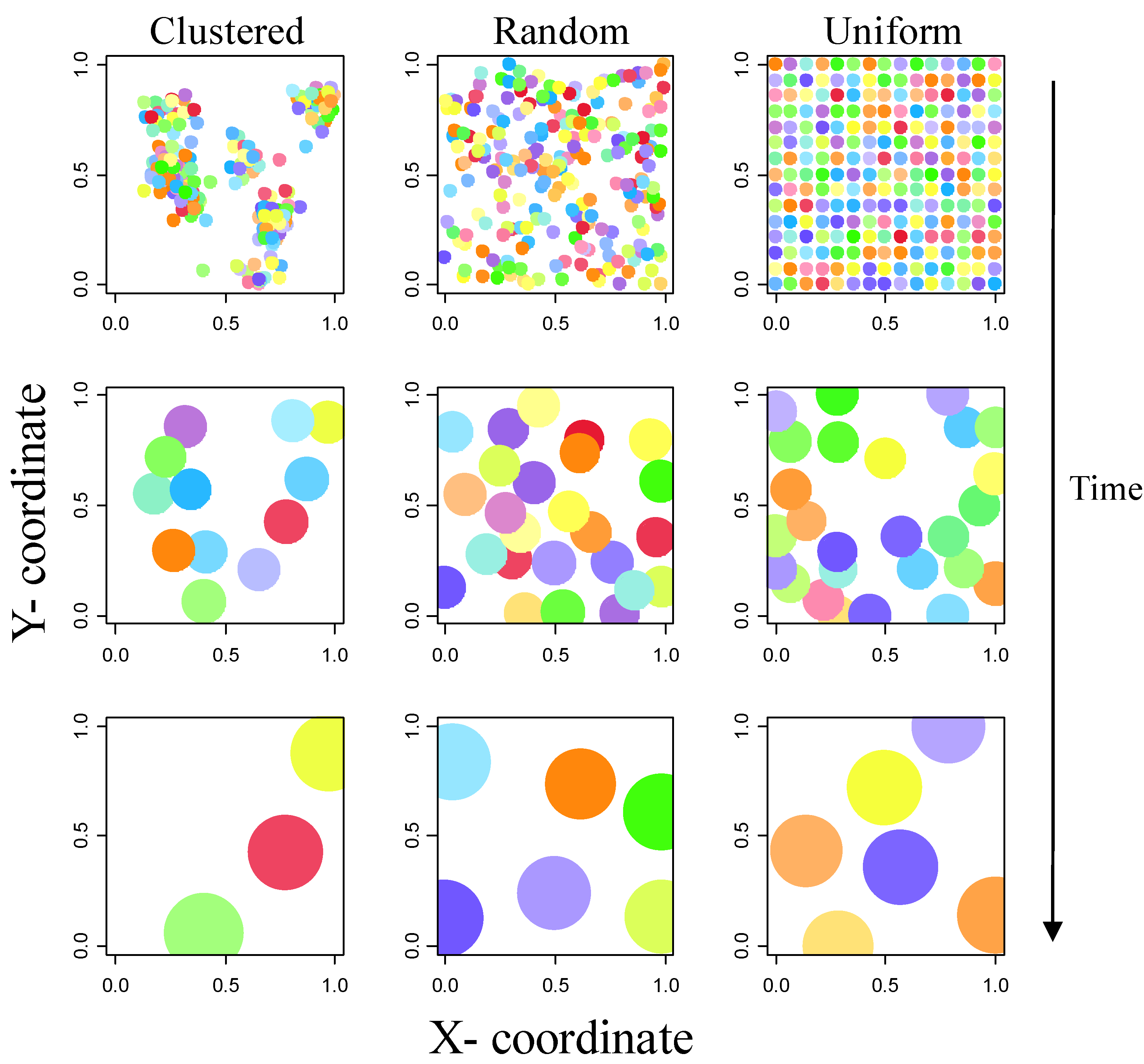
Individuals were placed on a 1 × 1 grid with a uniform, random, or clustered spatial distribution (Figure 1). We varied the number of individuals initially established exponentially from 25 to 225. This initial variation in the number of individuals is responsible for the ascending limb of the richness-biomass relationship in our model. We generated a new independent spatial distribution of individuals for each run of the model. The uniform spatial distribution was constructed by spacing each individual a fixed interval apart on the grid. The random spatial distribution was constructed by assigning the coordinates of individuals using a random uniform distribution. The clustered spatial distribution was generated by distributing the centers of the clusters according to a random uniform distribution and then normally distributing the individuals around each of the clusters. We arbitrarily set the number of cluster centers equal to 5% of the total number of individuals to achieve a high degree of clustering in the communities. The standard deviation of the normal distribution was set to the initial diameter of the individuals. This clustering process is similar but not identical to the popular Neyman-Scott point-process [14]. It is not a true Neyman-Scott point-process because individuals that were slated to become established outside of the 1 × 1 grid were reassigned to a new spatial cluster; additionally, the number of clusters was not a Poisson variable because it was always equal to 5% of the total number of individuals. Due to our boundary restrictions the clusters located in the center of the landscape had a slightly higher number of individuals.
At stand establishment all individuals were assigned the same starting diameter. The relative abundance distribution (RAD) of the species pool was set to uniform such that each species was equally likely to be drawn with replacement from the pool. Although a uniform RAD is not common in nature, more realistic RADs that contain more rare species (e.g., log normal and geometric distributions) simply compressed the richness-biomass relationship along the y-axis by decreasing the mean number of species in the community and did not influence the overall qualitative shape of the relationship (results not shown). Species were drawn with replacement randomly from the species pool.
Figure 1. A top-down view of simulated communities at three points in time: 1, 15, and 30. Each column of the panel depicts the results for a different initial spatial distribution: clustered, random, or uniform. Each circle represents an individual, the color of the circle indicates the species identity, and the area of the circle is equal to the area that the individual occupied in the 1 × 1 window. The same number of individuals was in each community initially.
Diversity 02 00550 g001

2.2. Growth Phase

Once individuals were established they were allowed to grow radially. Each individual increased its own diameter at a maximum rate unless it was overlapping any of its neighbors, in which case that individual’s growth decreased relative to the summed diameters of the overlapping individuals.
Diversity 02 00550 i001
Where ΔDi is the new diameter grow rate of individual i, ΔDmax is the maximum growth rate, N is the number of overlapping individuals, and Dj is the diameter of one of the overlapping neighbors. We also examined the effect of substituting Diversity 02 00550 i002 with Diversity 02 00550 i003 in equation 1, where Aij is area of overlap between individual i and its neighbor j. However, this change did not fundamentally alter the patterns, and it increased computation time by a factor of three. Therefore, we only present the results based upon the summed diameters of neighbors.

2.3. Thinning Phase

Here, we assume that mortality in the thinning phase is linked to slow growth caused by intense inter-individual competition. The probability that an individual would die was linearly related to the ratio of the actual growth to the maximum growth rate:
Diversity 02 00550 i004
where pi is the probability of mortality of individual i. Thus pi was modeled as a negative non-linear function of the summed diameters of the overlapping neighbors. If pi was greater than a random uniform deviate between 0 and 1 then the individual was killed otherwise the individual remained on the landscape.
Once the growth and thinning phases were complete, biomass was calculated using the allometric relationship between this variable and individual stem diameter, B α D8/3. The exponent of 8/3 is theoretically predicted by the metabolic theory of ecology and has received some empirical support [e.g., 15,16]. Therefore, total biomass, BT, was the sum of each individuals’ diameter raised to the 8/3 power,
Diversity 02 00550 i005
We also examined an allometric exponent of 2 which is supported empirically for some species of herbaceous plants [e.g., 17], but this did not qualitatively change our results and therefore will not be described further. Individuals were allowed to expand their diameters outside the bounds of the window but no individuals were rooted outside the window. During a single simulation run the establishment phase took place initially and then 50 growth and thinning phases took place.
Our simulation was written in R v.2.9.2 [18] and the script to run the simulation is provided in Appendix A. Here we present the results of our simulation model under a uniform RAD, but the R script provides the ability to examine the relationship for other RADs: log-normal, geometric, and an extremely uneven RAD. Furthermore, the script provides the ability to examine the influence of summed areas of overlap with neighbors rather than the summed diameters, a linear relationship between mortality and competition due to crowding, and different allometric exponents which specify the conversion of diameter to above-ground biomass.

3. Results

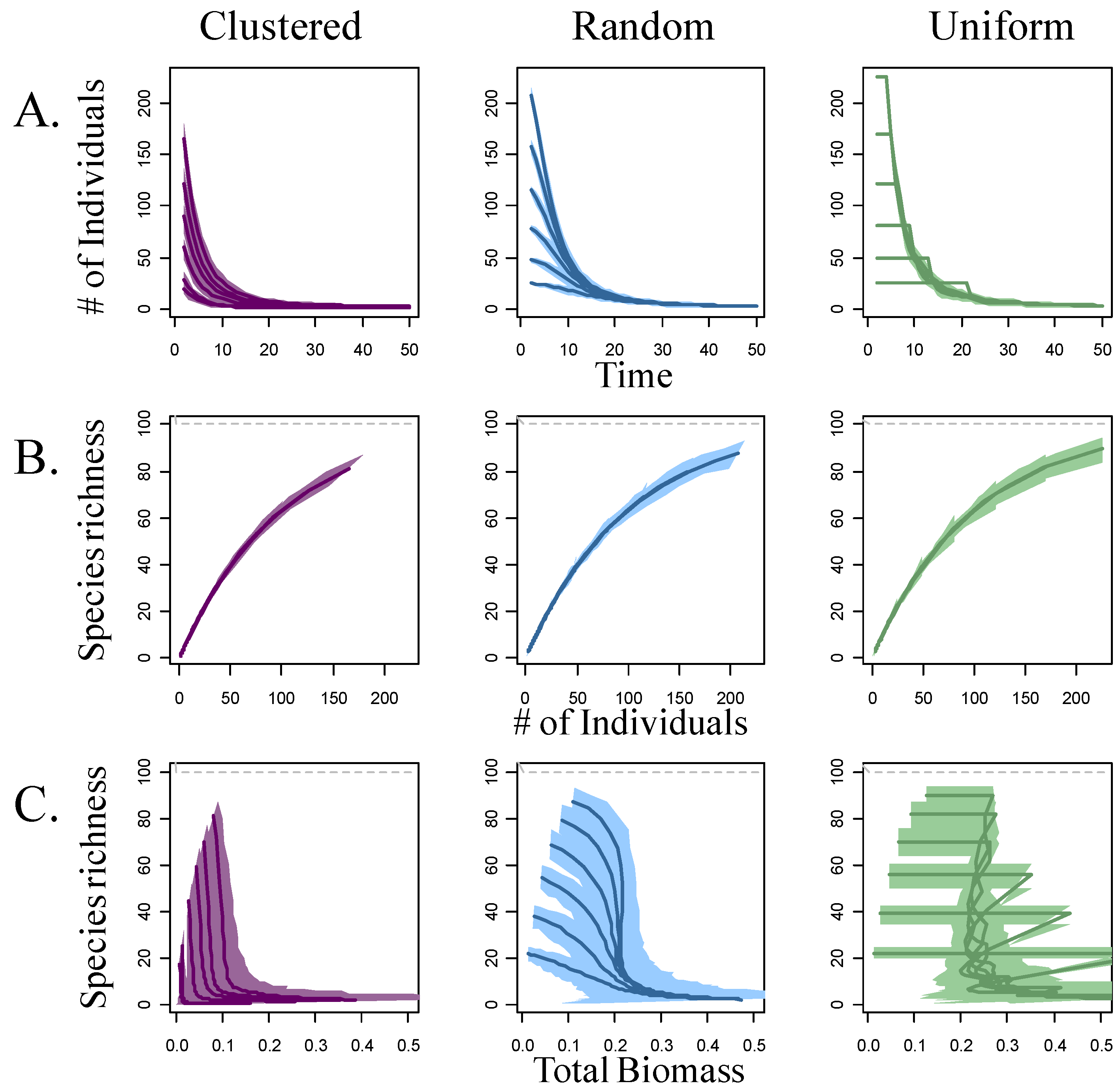
The averaged output of the simulation model is displayed in Figure 2. Each curve is the average of 200 independent trials and each represents the trajectory of a community through time that began with a particular number of individuals. We omitted the first time state (time = 1) from the graphical output of the simulation because thinning had not yet had a chance to occur. Across the three spatial distribution treatments, communities that started with more individuals had more species, a steeper rate of thinning, and an earlier onset of thinning. These effects in turn resulted in communities that displayed steeper negative relationships between biomass and richness. The initial spatial distribution of individuals had the strongest influence early in the simulation on the rate of thinning in a community and in the shape of the richness-biomass relationship. As time progressed the community patterns in the three spatial treatments converged (Figure 2).
Figure 2. Three bivariate relationships generated by the simulation model are illustrated below. As in Figure 1, each column of the panel depicts the results for a different initial spatial distribution. Each line represents the average trajectory of 200 trials for a community with a given initial number of individuals. The 95 % confidence envelopes are provided around each average line (the shaded regions around the curves). Each row of the figure illustrates a different relationship: (a) the decrease in the number of individuals through time, (b) the monotonic relationship between the number of individuals in a community and species richness, and (c) the richness-biomass relationship. The dotted grey line that appears in B and C indicates the size of the species pool.
Diversity 02 00550 g002
The averaged richness-biomass relationships all follow a negative monotonic temporal trajectory (Figure 2C); however, if we consider the entire ensemble of curves (i.e., all starting densities) it becomes clear that each spatial treatment resulted in a unimodal richness-biomass relationship. The clustered spatial distribution led to an earlier initiation of thinning and initially a more rapid thinning rate (Figure 2A). This resulted in fewer individuals and thus fewer species early on in the simulation which effectively resulted in a richness-biomass relationship with a sharper peak that was located at a lower level of total biomass (Figure 2C). The random spatial distribution displayed a richness-biomass relationships with a softer peak, but richness still declined rapidly in this community type when biomass was larger than approximately 0.2 (with the parameterizations given in Table 1). The richness-biomass relationship displayed distinct growth and thinning phases in the uniform spatial treatment. The growth phase was visible as a prominent initial plateau which was followed by rapid and episodic thinning. The two distinct phases were formed in the uniform community because individuals appeared to grow unencumbered by their neighbors until a threshold was crossed and thinning was initiated. This sudden initiation of mortality caused decreases in total biomass. This was particularly true of the uniform communities with few individuals initially (Figure 2A, C).
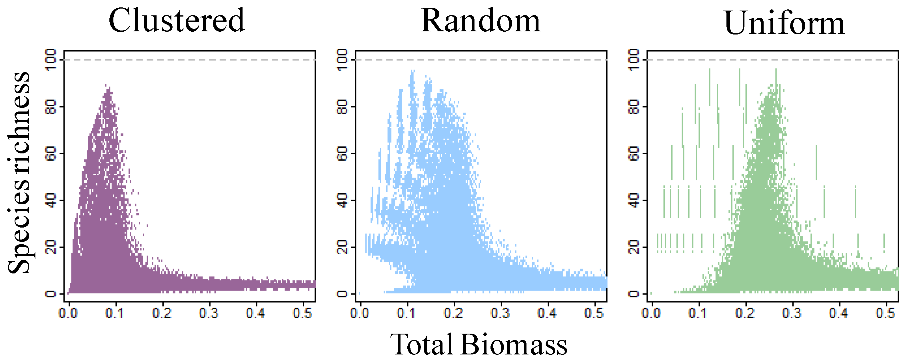
The unaveraged richness-biomass relationship provided two complementary results when examined outside of the temporal context (i.e., ignoring community trajectories through time, Figure 3). Specifically, the spatial treatments resulted in dense clouds of points that appeared to gradate into one another. Additionally, if we focus on only the periods in which thinning was occurred, it appeared that the uniform spatial distribution displayed the sharpest peak in richness.
Figure 3. The unaveraged richness-biomass relationship for 200 simulation runs. Each point represents the state of a single community at a point in time. The dotted grey line indicates the size of the species pool.
Diversity 02 00550 g003

4. Discussion

The objective of our study was to examine whether the initial spatial distribution of individuals influenced the richness-biomass relationship. Our results suggested that the spatial treatments resulted in distinct temporal trajectories along the richness-biomass relationship (Figure 2). Specifically, increasing the spatial uniformity of the population effectively shifted the location of the diversity peak to higher levels of total biomass. Additionally, the temporal community trajectories suggested that spatial clustering resulted in a sharp diversity peak, randomly distributing individuals was linked with a softer diversity peak, and the uniformly distributed scenario exhibited a flat-topped richness-biomass relationship. However when viewed outside of a temporal context, it is clear that the spatial treatments produced overlapping richness-biomass relationships that smoothly gradate into one another, and the uniformly distributed populations actually appeared to display the sharpest diversity peak, when we ignore the periods of no mortality.
The differences in the shape of the richness-biomass relationship were most apparent early in the simulation because as thinning progressed the communities converged to states in which they all possessed a few widely spaced individuals, few species, and the maximum levels of biomass (Figure 1 and Figure 2). The progression of the communities towards low diversity high biomass states took place in a relatively smooth and regular manner in the clustered and random communities but was more erratic in the uniform community due to the intense pulses of mortality that occurred in this community.

4.1. Self-thinning and Models of the Richness-Biomass Relationship

Although the influence of initial spatial arrangement of individuals has not been previously recognized in studies linking thinning and the richness-biomass relationship, studies that have more directly examined the phenomena of self-thinning in forests and herbaceous communities have recognized the importance of neighbor spacing for some time [e.g., 19,20]. Ross and Harper [21] found that initial density of neighbors had a strong effect on growth of individuals, second only to the effect of time-of-germination. The constant of the well known -3/2 thinning law is also thought to respond to spatial arrangement of individuals [22]. Guan et al. [23] found lower growth and higher mortality rates in stands of Japanese cedar (Cryptomeria japonica) that were grown more closely together. Furthermore, it makes intuitive sense that thinning should initiate earlier in situations in which individuals are on average more spatially proximate initially (i.e., spatially clustered).
The importance of considering individual density when modeling the richness-biomass relationship has received varying degrees of support experimentally, but the general consensus appears to be that the rarefaction effect provides a necessary null expectation for the behavior of the richness-biomass relationship. Several fine-scale experimental studies have demonstrated that the richness-biomass relationship responds strongly to rarefaction effects [12,24,25]. Additionally, Chiarucci et al. [25] demonstrated that competitive exclusion and the rarefaction effect are likely operating simultaneously in herbaceous communities. In two studies using the same experimentally manipulated alpine plant community, Luo et al. [26] and Niu et al. [27] found that although approximately 30–40% of the variance in richness was explained by the density of individuals, other community patterns such as the community similarity and patterns of biomass allocation in individual plants did not appear to support the assumption of species neutrality upon which the rarefaction effect is based.
The clonal nature of many plants may obscure the importance of rarefaction effects on the richness-biomass relationship [28], as well as, make it logistically infeasible to quantify individual density empirically [5,8]. In communities dominated by clonal plants it is increasingly difficult to distinguish individuals and spatial patterns of clumping are clearly not independent of species identity (as assumed by our model). Despite these additional challenges that clonality presents, the signature of rarefaction on patterns of richness should still be present but increasingly difficult to detect.
None of the studies examining the influence of individual density on the richness-biomass relationship demonstrate that the rarefaction effect explains all of the variance in the diversity-biomass relationship, but simply that the influence of individual density cannot be ignored. We would like to add to this general sentiment, that the initial spatial arrangement of individuals in the community may have important influences on the patterns of community thinning and consequently the shape of the richness-biomass relationship as well. Specifically, we suggest that a rigid boundary between the establishment and thinning phases exists primarily when individuals are distributed uniformly and thus initially experience a period of unencumbered growth. This finding suggests that Oksanen’s [10] NIM may best apply to communities with uniform spatial distributions, and that the ALT model of Stevens and Carson [12,13] may be more relevant to communities in which individuals are clustered or randomly distributed in space.

4.2. Applicability and Limitations of the Simulation Model

We designed our simulation model simply such that the results would be applicable to many different sessile organisms. As such our model is a tool for exploring qualitative differences in richness-biomass relationships and not a precise predictive model; therefore, we feel that it was acceptable to ignore additional complexities relating to organism dispersal, establishment, growth, and competition in the model. That being said, ignoring these complexities prevents our model from being calibrated to natural systems to provide estimates of richness at empirical levels of total biomass. It is important to note that our model focuses primarily on how community thinning influences the richness-biomass relationship, and therefore it may not adequately characterize the ascending limb of the unimodal relationship which we modeled simply by varying the initial number of individuals in the community. Additionally although the average richness-biomass relationships responded distinctly to the spatial treatments, in natural systems spatial patterns of establishment may be determined by a non-stationary process (i.e., the mean and variance of the process is not constant), which will add noise to the empirical richness-biomass relationship. Furthermore, the unaveraged values from the simulation indicate that the spatial treatments produced overlapping richness-biomass relationships that smoothly gradate into one another (Figure 3).
Although our simulation model is based upon temporal dynamics, the results need not be limited to temporal community patterns [29]. Spatially segregated samples from a single point in time have the potential to test predictions of the model and provide further empirical examination of the process of community thinning on the richness-biomass relationship. This is particularly true for empirical settings in which it is believed that different sites are undergoing similar temporal dynamics but are out of phase with one another due to an extrinsic environmental variable such as time since disturbance or site productivity.
Given the amount of scatter in many empirical richness-biomass relationships [e.g., 13,30], it will likely be difficult to attribute a particular curve shape to the influence of spatial patterning. Possibly the most revealing aspect of our simulation results is the demonstration of the potential diversity of unimodal richness-biomass relationships that can be attributed to community-thinning. Furthermore, it may be beneficial to interpret the dense clouds of points in Figure 3 as constraint spaces which suggest that at low biomass a wide range of richness values are possible, but at high total biomass richness must be low. Huston [31] suggested a similar line of reasoning when interpreting the negative relationships he observed between tropical tree richness and soil nutrient levels.

Supplementary Files

Supplementary File 1Supplementary File 2

Acknowledgements

DJM acknowledges post-doctoral support from Allen Hurlbert and additional funding from the U.S. Environmental Protection Agency (EPA) under the Greater Research Opportunities (GRO) Graduate Program. The U.S. EPA has not officially endorsed this publication, and the views expressed herein may not reflect the views of the Agency. MWP acknowledges support from NSF Grant Number EPS-0447262 and EPS-0919466.

References and Notes

  1. Grime, J.P. Competitive exclusion in herbaceous vegetation. Nature 1973, 242, 344–347. [Google Scholar] [CrossRef]
  2. Shipley, B.; Keddy, P.A.; Gaudet, C.; Moore, D.R.J. A model of species density in shoreline vegetation. Ecology 1991, 72, 1658–1667. [Google Scholar] [CrossRef]
  3. Gotelli, N.J.; Colwell, R.K. Quantifying biodiversity: procedures and pitfalls in the measurement and comparison of species richness. Ecol. Lett. 2001, 4, 379–391. [Google Scholar] [CrossRef]
  4. Gotelli, N.J.; Graves, G.R. Null Models in Ecology; Smithsonian Institution: Washington, DC, USA, 1996. [Google Scholar]
  5. McGlinn, D.J.; Palmer, M.W. Modeling the sampling effect in the species-time-area relationship. Ecology 2009, 90, 836–846. [Google Scholar] [CrossRef]
  6. Turner, W.R.; Tjørve, E. Scale-dependence in species-area relationships. Ecography 2005, 28, 721–730. [Google Scholar]
  7. Conner, E.F.; McCoy, E.D. The statistics and biology of the species-area relationship. Am. Nat. 1979, 113, 791–833. [Google Scholar]
  8. Palmer, M.W.; McGlinn, D.J.; Fridley, J.F. Artifacts and artifictions in biodiversity research. Folia Geobot. 2008, 43, 245–257. [Google Scholar] [CrossRef]
  9. Palmer, M.W.; Clark, D.A.; Clark, D.B. Is the number of tree species in small tropical forest plots nonrandom? Community Ecol. 2000, 1, 95–101. [Google Scholar] [CrossRef]
  10. Oksanen, J. Is the humped relationship between species richness and biomass an artefact due to plot size? J. Ecol. 1996, 84, 293–295. [Google Scholar] [CrossRef]
  11. Hubbell, S.P. The Unified Neutral Theory of Biodiversity and Biogeography; Princeton University Press: Princeton, NJ, USA, 2001. [Google Scholar]
  12. Stevens, M.H.H.; Carson, W.P. Plant density determines species richness along an experimental fertility gradient. Ecology 1999, 80, 455–465. [Google Scholar] [CrossRef]
  13. Stevens, M.H.H.; Carson, W.P. The significance of assemblage-level thinning for species richness. J. Ecol. 1999, 87, 490–502. [Google Scholar] [CrossRef]
  14. Fortin, M.J.; Dale, M. Spatial Analysis: A Guide for Ecologists; Cambridge University Press: Cambridge, UK, 2005. [Google Scholar]
  15. West, G.B.; Brown, J.H.; Enquist, B.J. A general model for the origin of allometric scaling laws in biology. Science 1997, 276, 122–126. [Google Scholar] [CrossRef]
  16. Pretzsch, H. Species-specific allometric scaling under self-thinning: evidence from long-term plots in forest stands. Oecologia 2006, 146, 572–583. [Google Scholar] [CrossRef]
  17. Niklas, K.J.; Cobb, E.D. Biomass partitioning and leaf N,P-stoichiometry: comparisons between tree and herbaceous current-year shoots. Plant Cell Environ. 2006, 29, 2030–2042. [Google Scholar] [CrossRef]
  18. R Development Core Team. R: A Language and Environment for Statistical Computing; R Foundation for Statistical Computing: Vienna, Austria, 2009. [Google Scholar]
  19. Kenkel, N.C. Pattern of self-thinning in jack pine: testing the Random Mortality Hypothesis. Ecology 1988, 69, 1017–1024. [Google Scholar] [CrossRef]
  20. Mack, R.N.; Harper, J.L. Interference in dune annuals: spatial pattern and neighbourhood effects. J. Ecol. 1977, 65, 345–363. [Google Scholar] [CrossRef]
  21. Ross, M.A.; Harper, J.L. Occupation of biological space during seedling establishment. J. Ecol. 1972, 60, 77–88. [Google Scholar] [CrossRef]
  22. White, J.; Harper, J.L. Correlated changes in plant size and number in plant populations. J. Ecol. 1970, 58, 467–485. [Google Scholar] [CrossRef]
  23. Guan, B.T.; Lin, S.-T.; Lin, Y.-H.; Wu, Y.-S. Growth efficiency-survivorship relationship and effects of spacing on relative diameter growth rate of Japanese cedars. For. Ecol. Manage. 2008, 255, 1713–1723. [Google Scholar] [CrossRef]
  24. Goldberg, D.E.; Miller, T.E. Effects of different resource additions on species diversity in an annual plant community. Ecology 1990, 71, 1990. [Google Scholar]
  25. Chiarucci, A.; Alongi, C.; Wilson, J.B. Competitive exclusion and the No-Interaction model operate simultaneously in microcosm plant communities. J. Veg. Sci. 2004, 15, 789–796. [Google Scholar] [CrossRef]
  26. Luo, Y.J.; Qin, G.L.; Du, G.Z. Importance of assemblage-level thinning: A field experiment in an alpine meadow on the Tibet plateau. J. Veg. Sci. 2006, 17, 417–424. [Google Scholar] [CrossRef]
  27. Niu, K.C.; Luo, Y.J.; Choler, P.; Du, G.Z. The role of biomass allocation strategy in diversity loss due to fertilization. Basic Appl. Ecol. 2008, 9, 485–493. [Google Scholar] [CrossRef]
  28. Rajaniemi, T.K. Why does fertilization reduce plant species diversity? Testing three competition-based hypotheses. J. Ecol. 2002, 90, 316–324. [Google Scholar]
  29. Oksanen, J. The no-interaction model does not mean that interactions should not be studied. J. Ecol. 1997, 85, 101–102. [Google Scholar] [CrossRef]
  30. Grace, J.B. The roles of community biomass and species pools in the regulation of plant diversity. Oikos 2001, 92, 193–207. [Google Scholar]
  31. Huston, M. Soil nutrients and tree species richness in Costa Rican forests. J. Biogeogr. 1980, 7, 147–157. [Google Scholar] [CrossRef]