Responses of Soil Fauna Diversity to Management in the European Important Floodplain Habitats of the Danube

Abstract

Soil fauna represent an important component of terrestrial ecosystems and serve as sensitive bioindicators of environmental changes and the intensity of anthropogenic disturbances. Our research was conducted between 2020 and 2023 across 15 habitats differing in management intensity. Soil fauna were sampled using pitfall traps. A total of 88,112 individuals belonging to 18 taxa were recorded. Community variability was assessed using redundancy analysis (RDA), which revealed a clear differentiation between managed and unmanaged habitats. The results indicated that more soil fauna preferred more stable and less disturbed environments, whereas managed sites exhibited greater heterogeneity of soil fauna communities. Statistical analyses confirmed significant differences in individual abundance among study areas (1–15), years (2020–2023), and seasons (Friedman test, p = 0.016; Kruskal–Wallis test, p < 0.001), highlighting the substantial influence of habitat characteristics and seasonal dynamics on the structure of soil fauna. The predictive models suggested the persistence of natural population fluctuations without a pronounced long-term decline in abundance. The findings provide valuable information for optimizing habitat management, evaluating the effectiveness of restoration measures, and supporting biodiversity conservation in ecosystems of European importance.

1. Introduction

Floodplain ecosystems are among the most biologically valuable and, at the same time, the most threatened habitats in Europe. The Danube floodplain ecosystem represents one of the biodiversity hotspots of Central Europe, harboring approximately 2000 species of plants and more than 5000 animal species. They are characterized by high habitat heterogeneity, which creates suitable conditions for the occurrence of a wide range of plant and animal species, including soil fauna [1]. These organisms play an important role in ecosystem processes, particularly in the decomposition of organic matter, nutrient cycling, regulation of other invertebrate populations, and maintenance of soil fertility [2]. At the same time, they serve as sensitive bioindicators of disruptions to habitats and changes caused by anthropogenic activity and are therefore frequently used in assessing the ecological status of habitats and the effectiveness of management measures [3].

Floodplain habitats represent highly dynamic environments characterized by regular fluctuations in the hydrological regime, which significantly influence the structure and diversity of soil fauna. Periodic flooding not only causes direct changes in the abundance of individual taxa but also creates spatially heterogeneous conditions that lead to the formation of a wide range of ecological niches. Consequently, many soil fauna exhibit specific adaptive strategies that enable them to survive under conditions of fluctuating moisture and periodic inundation. Some species utilize vertical migration to higher vegetation layers or deeper soil horizons, while others are capable of rapidly colonizing newly available habitats following water recession [4]. Another important factor shaping soil fauna in floodplain ecosystems is the spatial heterogeneity of vegetation. The alternation of forest stands, wetlands, grasslands, and successional stages creates diverse microclimatic conditions that support the coexistence of species with different ecological requirements. Studies have shown that transitional zones between habitat types often exhibit higher diversity of soil fauna than homogeneous habitats because they provide a broader range of food resources, shelters, and reproductive opportunities [5]. This spatial heterogeneity is considered one of the principal factors responsible for the high biodiversity of floodplain ecosystems. The floodplain ecosystems of the Danube rank among the most important biodiversity hotspots in Central Europe, providing habitat for approximately 5000 animal species.

In recent decades, many floodplain forests and wetland habitats have been significantly affected by human activities, including river regulation, intensive agriculture, urbanization, and changes in land use. These interventions have led to habitat fragmentation, biodiversity loss, and the disruption of natural ecological processes [6,7,8]. In response to these negative trends, restoration and management measures aimed at recovering the ecological functions of floodplain ecosystems have been implemented in many countries. Research indicates that appropriately designed management practices can significantly promote the recovery of soil fauna diversity and enhance the ecological stability of these habitats [9,10].

Soil fauna respond very sensitively to environmental changes, with their abundance, species diversity, and spatial distribution being influenced by vegetation structure, microclimatic conditions, soil moisture, and the intensity of disturbances [11]. Several studies have confirmed that habitats with lower levels of anthropogenic disturbance provide more suitable conditions for maintaining stable and diverse soil fauna than intensively managed sites [12,13,14]. An important factor is also the seasonal dynamics of populations, which reflect the natural fluctuations of environmental conditions throughout the year and influence the activity patterns of individual soil fauna [15].

The aim of this study was to investigate the impact of habitat and management on soil fauna and to evaluate long-term trends. Hypothesis 1: Management affects abundance, diversity, and community composition. Hypothesis 2: Managed habitats support more stable and diverse communities. Hypothesis 3: LSTM will show that under current management there will be no long-term decline in populations.

2. Materials and Methods

During the years 2020–2023, research activities were conducted across 15 selected sampling sites, which belonged to 8 habitats. Two habitats were without management and eight with management, so we evaluated ten habitats. The survey took place in the Dunajské luhy Protected Landscape Area, a valuable floodplain ecosystem located in western Slovakia and designated as a territory of European ecological significance. The protected area covers approximately 122.8 km² and belongs to the Alpine–Himalayan biogeographical system situated within the Danubian Lowland. In terms of climate, the region is considered relatively warm, with generally moderate winter conditions. During 2020, the average spring temperature was 11 °C, the summer temperature was 21 °C, and the autumn temperature was 11 °C. During 2021, the average spring temperature was 9 °C, the summer temperature was 22 °C, and the autumn temperature was 11 °C. During 2022, the average spring temperature was 11 °C, the summer temperature was 22 °C, and the autumn temperature was 11 °C. During 2023, the average spring temperature was 10 °C, the summer temperature was 22 °C, and the autumn temperature was 14 °C. The geological base is mainly composed of clay-loam soils formed from alluvial sediments deposited by the Danube River.

Across the selected forest habitats (willow–poplar floodplain woodland, ash–alder inundated forest, Pannonian poplar stands, and reed-dominated wetland vegetation), various ecological restoration measures were implemented. These measures involved creating new side branches within the Danube Delta network and artificially inducing flood conditions twice each year, specifically during the spring and summer periods. In non-forest habitats (grazing areas, poplar plantations, floodplain grasslands, and lowland hay meadows), several additional management approaches were carried out. Vegetation between plantation rows was cut twice annually, in spring and summer. Meadow communities were mown once per year (at the end of May every year), selected meadow areas experienced seasonal flooding (in mid-June and late August every year), and extensive cattle grazing was preserved as an important component of habitat management.

Two habitat types, namely willow–poplar floodplain forest and native pasture, where no restoration interventions had been implemented, served as control sites. Willow–poplar floodplain habitat without management was represented in 3 study areas (S1–S3). Pasture habitat without management was represented in 1 study area (S4). Ash–alder floodplain forests with management habitat were represented in 1 study area (S5). Pannonian poplar forest with management habitat was represented in 1 study area (S6). Reed communities of wetlands with management habitat were represented in 1 study area (S7). Willow–poplar floodplain forest with management habitat was represented in 2 study areas (S8 and S14). Pasture habitat was represented in 1 study area (S9). Poplar nursery habitat was represented in 3 study areas (S10, S13, and S15). Lowland hay meadow with management habitat was represented in 1 study area (S11). Alluvial meadow with management habitat was represented in 1 study area (S12). The research was conducted in 15 study areas that belong to 8 habitats, which are listed in

Table 1. Location data study areas 1–15.

Study Areas	Habitat	Meters Above Sea Level	Geographic Coordinates	Management
S1	Willow–poplar floodplain forest	114	47°53′31.1″ N 17°30′25.4″ E	without management
S2	Willow–poplar floodplain forest	119	47°54′36.0″ N 17°27′51.3″ E	without management
S3	Willow–poplar floodplain forest	106	47°45′17.0″ N 17°56′59.9″ E	without management
S4	Pasture	108	47°45′09.3″ N 17°56′58.8″ E	without management
S5	Ash–alder floodplain forests	121	47°58′27.4″ N 17°22′09.1″ E	with management
S6	Pannonian poplar forest	121	47°58′27.4″ N 17°22′09.1″ E	with management
S7	Reed communities of wetlands	121	47°58′41.6″ N 17°22′03.7″ E	with management
S8	Willow–poplar floodplain forest	114	47°53′31.5″ N 17°30′30.2″ E	with management
S9	Pasture	119	47°54′33.8″ N 17°27′52.6″ E	with management
S10	Poplar nursery	118	47°53′51.5″ N 17°27′25.5″ E	with management
S11	Lowland hay meadow	110	47°47′07.2″ N 17°44′11.4″ E	with management
S12	Alluvial meadow	108	47°45′00.0″ N 17°56′09.2″ E	with management
S13	Poplar nursery	108	47°44′48.3″ N 17°55′20.2″ E	with management
S14	Willow–poplar floodplain forest	115	47°53′28.5″ N 17°28′56.9″ E	with management
S15	Poplar nursery	127	47°58′22.9″ N 17°22′02.9″ E	with management

.

The botanical description of the study areas is as follows:

Study area 1 (SA1) = willow–poplar floodplain forest (reference habitat where no revitalization measures were carried out). The tree layer was formed by the species Salix fragilis Linnaeus (1753) and Salix alba Crawford (1914). The herbaceous layer was represented by species Urtica dioica Linné (1753), Impatiens glandulifera Royle (1834), Solidago gigantea Aiton. (1789), Galium odoratum Fl. Carniol (1771), Parietaria officinalis Linnaeus (1753), Rubus caesius Linnaeus (1753), Stachys sylvatica Linnaeus (1753), and Lamium maculatum Linnaeus (1763).

Study area 2 (SA2) = willow–poplar floodplain forest (reference habitat where no revitalization measures were carried out). The tree layer was formed by the species S. alba, S. fragilis, Populus × canadensis Moench (1785), Acer negundo Linnaeus (1753), Crataegus monogyna Jacquin (1775), and Populus × canescens Smith (1804). The shrub layer consisted of Sambucus nigra Linnaeus (1753), A. negundo, and Swida sanguinea Opiz (1852). The herb layer was represented by the species I. glandulifera, U. dioica, R. caesius, Valeriana officinalis Linnaeus (1753), Arctium nemorosum Lejeune (1833), Impatiens parviflora de Candolle (1824), Roegneria canina Nevski (1933), and Galium aparine Linnaeus (1753).

Study area 3 (SA3) = willow–poplar floodplain forest (reference habitat where no revitalization measures were carried out). The tree layer was composed of S. alba, S. fragilis, Populus alba Linnaeus (1753), P. × canescens, P. nigra, Alnus glutinosa Gaertn (1790), and A. negundo. The shrub layer consisted of S. nigra, Fraxinus excelsior Linnaeus (1753), A. negundo, S. sanguinea, and Corylus avellana Linnaeus (1753). The herb layer was represented by the species U. dioica, Phalaroides arundinacea Rauschert 1963, S. gigantea, Aster lanceolatus Nuttall (1818), R. caesius, and Humulus lupulus Linnaeus (1753).

Study area 4 (SA4) = pasture (original grassland, reference habitat where no revitalization measures were carried out). The tree layer consists of solitary individuals of S. alba. The herb layer was represented by the species U. dioica, Cirsium arvense Scopoli (1771), Eryngium campestre Linnaeus (1753), Achillea millefolium Linnaeus (1753), Crepis biennis Linnaeus (1753), Plantago lanceolatum Linnaeus (1753), P. major, Rumex crispus Linnaeus (1753), Elytrigia repens Nevski (1933), Dactylis glomerata Linnaeus (1753), Arrhenatherum elatius Presl & Presl (1819), Cichorium intybus Linnaeus (1753), Carduus acanthoides Linnaeus (1753), Trifolium repens Linnaeus (1753), Ranunculus repens Linnaeus (1753), Euphorbia palustris Linnaeus (1753), Eryngium planum Linnaeus (1753), Centaurea jacea Linnaeus (1753), and Setaria pumila Roemer & Schultes (1817).

Study area 5 (SA5) = ash–alder floodplain forest (forest habitat where revitalization measures were carried out = expansion of the branches of the Danube delta on the biotope, simulated flooding). The tree layer was composed of P. alba, P. × canescens, Acer campestre Linnaeus (1753), and A. negundo. The shrub layer consisted of F. excelsior, S. sanguinea, and Ligustrum vulgare Linnaeus (1753).

Study area 6 (SA6) = Pannonian poplar forest (forest habitat where revitalization measures were carried out = expansion of the branches of the Danube delta on the biotope, simulated flooding). The tree layer was formed by Populus nigra Linnaeus (1753), P. alba, and S. alba. The herb layer was represented by the species U. dioica, R. caesius, G. aparine, R. canina, S. gigantea, D. glomerata, E. repens, and Stenactis annua Nees (1832).

Study area 7 (SA7) = willow–poplar floodplain forest (forest habitat where revitalization measures were carried out = expansion of the branches of the Danube delta on the biotope, simulated flooding). The tree layer was composed of S. fragilis and S. alba. The herb layer was represented by the species U. dioica, I. glandulifera, S. gigantea, G. odoratum, P. officinalis, R. caesius, S. sylvatica, and L. maculatum.

Study area 8 (SA8) = willow–poplar floodplain forest (forest habitat where revitalization measures were carried out = expansion of the branches of the Danube delta on the biotope, simulated flooding). The tree layer was composed of P. × canadensis, P. robusta, S. fragilis, and Viscum album Linnaeus (1753). The shrub layer consisted of S. nigra, Cornus sanguinea Linnaeus (1753), and A. negundo. The herb layer was represented by the species Phragmites australis Steudel (1841), U. dioica, G. aparine, Ficaria bulbifera Holub (1961), Carduus crispus Linnaeus (1753), Symphyotrichum lanceolatum Nesom (1995), R. caesius, I. glandulifera, Sparganium erectum agg. Linnaeus (1753), Arctium sp. Linnaeus (1753), H. lupulus, Galeopsis speciosa Miller (1768), and Cucubalus baccifer Linnaeus (1753).

Study area 9 (SA9) = reed communities of wetlands (the edge of a wetland directly connected to a forest habitat, where revitalization measures were carried out = expansion of the branches of the Danube delta on the biotope, simulated flooding). The tree layer was composed of S. alba, P. × canadensis, and A. negundo. The herb layer was represented by the species P. australis, U. dioica, Lythrum salicaria Linnaeus (1753), R. caesius, and S. gigantea.

Study area 10 (SA10) = poplar nursery (planted poplar nursery where revitalization measures were carried out = expansion of the branches of the Danube delta on the biotope, simulated flooding). The study area was planted with P. alba and P. × canescens. It was a 2-year-old stand without a tree or shrub layer. The herb layer was represented by the species R. caesius, S. gigantea, P. alba, S. sanguinea agg., A. lanceolatus, U. dioica, Chenopodium album Linnaeus (1753), Symphytum officinale Linnaeus (1753), Stellaria media Villars (1789), Geum urbanum Linnaeus (1753), Erigeron annuus Persoon (1807), and E. repens.

Study area 11 (SA11) = poplar nursery (planted poplar nursery where revitalization measures were carried out = expansion of the branches of the Danube delta on the biotope, simulated flooding). The study area was planted with P. alba and P. × canescens. It was a 2-year-old stand without a tree or shrub layer. The herb layer was represented by the species R. caesius, S. gigantea, P. alba, S. sanguinea agg., A. lanceolatus, U. dioica, Ch. album, S. officinale, S. media, G. urbanum, E. annuus, and E. repens.

Study area 12 (SA12) = poplar nursery (planted poplar nursery where revitalization measures were carried out = expansion of the branches of the Danube delta on the biotope, simulated flooding). The study area was planted with P. alba and P. × canescens. It is a 2-year-old stand without a tree or shrub layer. The herb layer was represented by the species R. caesius, S. gigantea, P. alba, S. sanguinea agg., A. lanceolatus, U. dioica, Ch. album, S. officinale, S. media, G. urbanum, E. annuus, and E. repens.

Study area 13 (SA13) = alluvial meadow (meadow habitat where revitalization measures were carried out = expansion of the branches of the Danube delta on the biotope, simulated flooding). Solitary individuals of Taraxacum sec. Ruderalia occurred within the study area. The herb layer was represented by the species A. millefolium, C. biennis, P. lanceolatum, P. major, E. repens, D. glomerata, A. elatius, C. intybus, T. repens, C. jacea, S. pumila, R. caesius, S. officinale, R. repens, R. acris, Leontodon autumnalis Oeder (1816), Thlaspi perfoliatum Linnaeus (1753), R. crispus, E. palustris, Iris pseudacorus Linnaeus (1753), and Galium boreale Linnaeus (1753).

Study area 14 (SA14) = lowland hay meadow (meadow habitat where revitalization measures were carried out = expansion of the branches of the Danube delta on the biotope, simulated flooding). The herb layer on the study area was represented by the species E. annuus, D. glomerata, C. intybus, Plantago media Linnaeus (1753), C. arvense, A. millefolium, E. repens, S. gigantea, Inula britannica Bieberstein (1808), and S. officinale.

Study area 15 (SA15) = pasture (grassland where revitalization measures were carried out = expansion of the branches of the Danube delta on the biotope, simulated flooding, grazing by cattle). Solitary individuals of S. alba occurred within the study area. The herb layer was represented by the species C. arvense, C. acanthoides, A. lanceolatus, Artemisia campestris Linnaeus (1753), U. dioica, R. caesius, Agropyron repens Beauvois (1812), Lactuca serriola Linnaeus (1756), Tanacetum vulgare Linnaeus (1753), Glechoma hederacea Linnaeus (1753), Stenactis annua Nees (1832), A. millefolium, Poa pratensis Linnaeus (1753), P. media, Potentilla reptans Linnaeus (1753), Picris hieracioides Linnaeus (1753), G. parviflora, and Verbena officinalis Linnaeus (1753).

Sampling of soil fauna assemblages was conducted using pitfall traps on a monthly basis from April to October during the years 2020–2023. Each year, pitfall traps were placed for 92 days during spring (March, April, May), 92 days during summer (June, July, August), and 91 days during autumn (September, October, November). We collected soil fauna material at monthly intervals. We subsequently sorted and identified the soil fauna material to the order level in the laboratory. All traps contained a 4% formalin (Central chem, Slovakia) solution as a preservative agent. At each study site, five pitfall traps were positioned in a straight line with 10 m distances between adjacent traps, resulting in a transect measuring 40 m in total length. In total, 75 traps were installed annually across all investigated localities. Pitfall traps were placed at ground level, and the opening was not protected by a canopy. The collection of soil fauna took place at monthly intervals. The volume of pitfall traps was 750 mL with a hole diameter of 6.5 cm.

Statistical Analyses

To examine the relationships between the composition of soil fauna and study areas (1–15) with management, redundancy analysis (RDA) was employed. This ordination approach was chosen according to the length of the first ordination gradient (SD = 1.1), which suggested that soil fauna was related to environmental factors (years, seasons, management). We used logarithmic transformation of the data due to data heterogeneity. The dataset consisted of abundance and occurrence records of soil fauna obtained from both managed habitats and reference habitats without management intervention. We tested the significant influence of environmental variables using the Monte Carlo permutation test. The ordination procedure was applied to determine the principal gradients driving variability in soil fauna composition and to evaluate the relationships between particular species, study areas (1–15), years, seasons, and management types. Interpretation of the results was based on the spatial arrangement of sampling sites and the orientation of species vectors within the ordination diagram. All analyses were conducted using Canoco5 software (Microcomputer Power, Ithaca, NY, USA, 2012) [16].

The normality of data distribution was assessed using the Shapiro–Wilk test. Differences in the abundance of individuals among study areas (1–15), years (2020–2023), and seasons were first evaluated using the Friedman test. Subsequently, differences in abundance between study areas (1–15), years (2020–2023), and seasons were analysed separately using the Kruskal–Wallis test. Differences in the number of individuals between management types were tested by the Mann–Whitney U test. Statistical significance was determined at the α = 0.05 level. By multiple comparison of samples, pairwise comparisons among study area (1–15), year (2020–2023), and season (spring, summer, autumn) combinations were performed using Dunn’s post hoc multiple comparison test with Holm correction for multiple testing. Future trends in the number of individuals were predicted using a Long Short-Term Memory (LSTM) model, a type of neural network suitable for time-series analysis. The model was trained on historical abundance data for 250 epochs. Prediction accuracy was evaluated using the Mean Absolute Percentage Error (MAPE) metric. All statistical analyses were performed using Python 3.12. (Python Software Foundation, Beaverton, OR, USA, 2023) [17]. In the PAST 3 program (Hammer, Natural History Museum, University of Oslo, Oslo, Norway, 2017) [18], we calculated the Shannon diversity index (H′).

3. Results

The studied habitats exhibited substantial differences in both the abundance and taxonomic composition of soil fauna. In total, 88,112 individuals belonging to 18 soil fauna were recorded. The highest abundances were observed in Collembola (28.69%), Coleoptera (18.41%), Isopoda (10.77%), Hymenoptera (9.10%), and Araneae (8.93%).

The highest total number of individuals was recorded in the willow–poplar floodplain forest without management interventions (20.89%) and in the willow–poplar floodplain forest with management (18.84%), highlighting the importance of stable and less disturbed habitats for the maintenance of rich soil fauna. In contrast, the lowest abundance was observed in the pasture with management interventions (0.76%) and in the poplar nursery (2.06%), which may be associated with more intensive anthropogenic disturbance and lower ecological stability of these environments (

Table 2. Overview of soil fauna obtained from the investigated habitats. Explanations: A = pasture, B = willow–poplar floodplain forest (without management), C = pasture, D = willow–poplar floodplain forest, E = ash–alder floodplain forests, F = Pannonian poplar forest, G = reed communities of wetlands, H = poplar nursery, I = alluvial meadow, J = lowland hay meadow (with management).

Class	Order	Without Management		With Management								∑ Individuals	%
		A	B	C	D	E	F	G	H	I	J
Arachnoidea	Scorpionida	0	20	0	10	6	143	0	0	6	0	185	0.21
	Opilionida	22	373	1	634	90	93	19	5	105	31	1373	1.56
	Araneida	1486	879	11	1548	670	706	505	624	1052	390	7871	8.93
	Acarina	42	1112	2	1333	94	64	25	0	182	93	2947	3.35
Malacostraca	Isopoda	129	2354	11	2083	958	1062	159	6	1689	1036	9487	10.77
Chilopoda	Lithobiomorpha	65	619	3	743	294	300	99	9	457	379	2968	3.37
	Geophilomorpha	0	0	0	3	0	0	0	0	0	0	3	0.01
Diplopoda	Julida	143	1406	22	970	220	272	254	22	705	312	4326	4.91
	Polydesmida	28	409	1	499	68	46	0	0	117	15	1183	1.34
	Glomerida	100	624	0	449	165	333	0	0	217	134	2022	2.30
Parainsecta	Collembola	2360	5826	0	4143	4418	2917	740	0	2217	2658	25,279	28.69
Insecta	Thysanura	0	2	0	0	0	1	0	0	0	0	3	0.01
	Dermaptera	454	143	1	7	117	122	41	0	480	233	1598	1.81
	Orthoptera	291	49	0	185	127	175	78	25	373	174	1477	1.68
	Hemiptera	362	940	0	588	315	310	59	3	434	132	3143	3.57
	Auchenorrhyncha	0	2	0	1	0	0	0	0	0	0	3	0.01
	Coleoptera	645	2262	598	1477	3202	3393	805	1048	1955	839	16,224	18.41
	Hymenoptera	743	1384	19	1924	825	748	479	69	1611	218	8020	9.10
∑ individuals		6870	18,404	669	16,597	11,569	10,685	3263	1811	11,600	6644	88,112	100

).

The Shannon diversity index (H′), calculated at the order level, revealed considerable differences in the diversity of soil fauna communities among the individual study areas. The highest values were recorded at SA8 (H′ = 2.337), SA2 (H′ = 2.309), SA15 (H′ = 2.301), SA10 (H′ = 2.279), and SA14 (H′ = 2.210), indicating high taxonomic diversity and a relatively even distribution of individual orders. In contrast, the lowest values were found at SA9 (H′ = 0.497), SA13 (H′ = 0.881), and SA12 (H′ = 0.993), where the communities were characterized by the dominance of only a few taxonomic groups. Among the unmanaged habitats, willow–poplar floodplain forests showed considerable variation in diversity, with the highest value recorded at SA2 (H′ = 2.309), followed by SA1 (H′ = 2.045), whereas SA3 (H′ = 1.490) exhibited substantially lower diversity. The unmanaged pasture (SA4; H′ = 1.962) reached diversity values comparable to those of several managed forest habitats. Among the managed forest sites, the highest diversity was observed at SA8, while SA5 (H′ = 1.816), SA6 (H′ = 1.990), and SA7 (H′ = 1.971) displayed intermediate values. Marked differences were also found among the poplar nursery sites, where SA10 (H′ = 2.279) and SA11 (H′ = 1.988) exhibited high diversity, whereas SA12 (H′ = 0.993) ranked among the least diverse sites. Overall, the results indicate that forest habitats, particularly floodplain forests, support higher taxonomic diversity of soil fauna, whereas reed communities and some managed open habitats are characterized by lower taxonomic diversity.

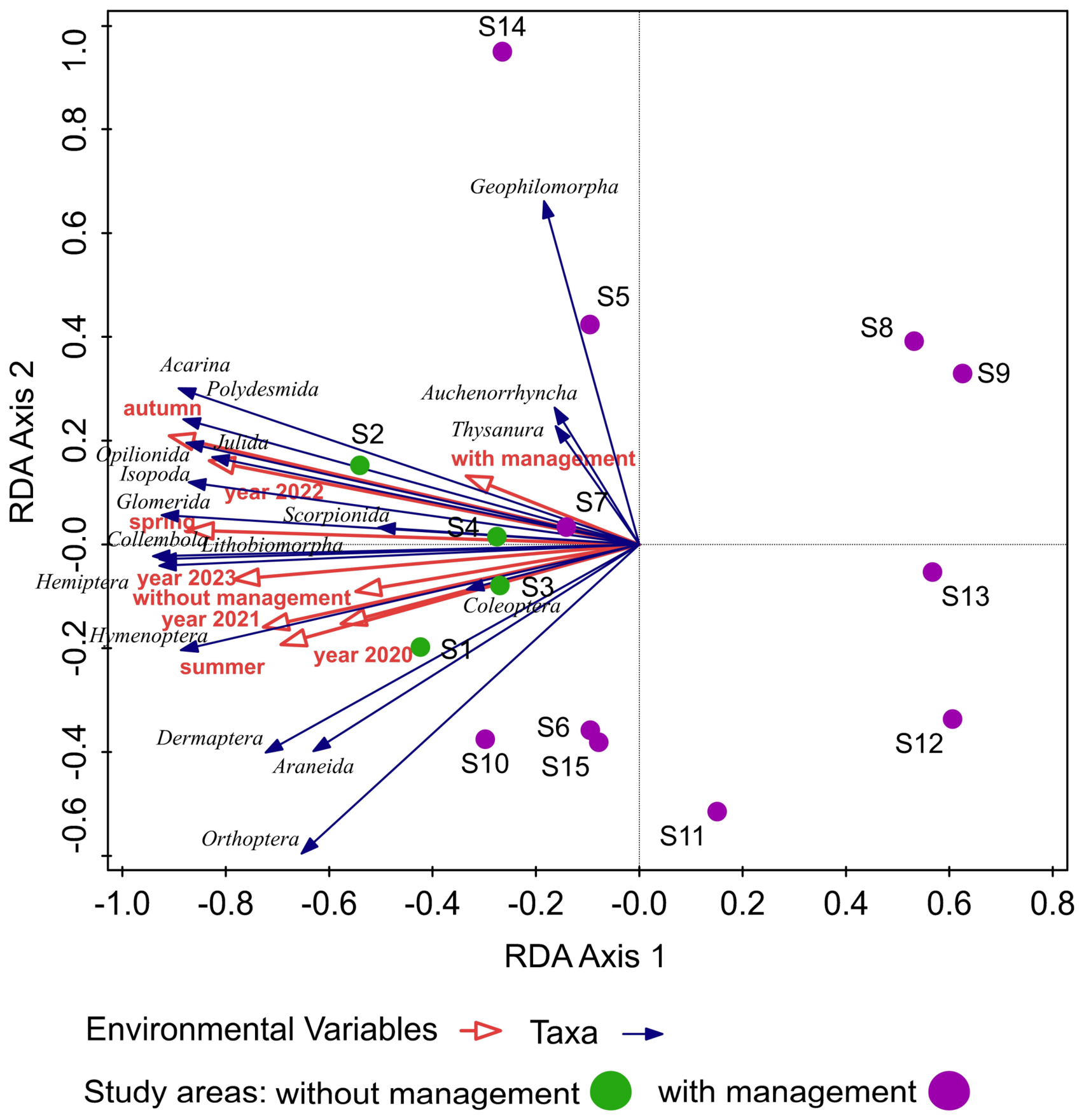
We used the redundancy analysis (SD = 1.1 on the first ordinate axis) to analyze the impact of management (with management, without management) on the spatial dispersion of soil fauna in the studied habitats. The values of the explained cumulative variability of taxon data were 72.77% on the first ordinate axis and 78.76% on the second ordinate axis. Due to the impact of land use, the variability on the first ordinate axis increased to 84.34%, and on the second cumulative axis, there was an increase to 91.29%. A significant impact on the spatial distribution of epigeic soil fauna was confirmed in environmental variables autumn (p = 0.002), spring (p = 0.002), summer spring (p = 0.012), year 2020 (p = 0.046), year 2021 (p = 0.002), year 2022 (p = 0.002), year 2023 (p = 0.002), with management (p = 0.032), and without management (p = 0.028).

The RDA analysis revealed a clear differentiation of the study areas according to management practices. The unmanaged sites (SA1–SA4) formed a compact cluster on the left side of the ordination space, indicating a similar structure of soil fauna communities and relatively stable environmental conditions. In contrast, the managed sites (SA5–SA15) were dispersed across a larger portion of the ordination diagram, reflecting greater spatial heterogeneity of the communities resulting from the implemented restoration measures. The most distinct sites were SA8, SA9, SA12, SA13, and SA14, which exhibited a specific taxonomic composition. Site SA7 occupied an intermediate position between the unmanaged and managed areas, suggesting a transitional community structure. In contrast, sites SA6, SA10, SA11, and SA15 formed a separate group in the lower part of the ordination space, distinguished primarily by the composition of the dominant soil fauna.

From a trophic perspective, the RDA analysis indicated that individual trophic groups responded differently to management practices. Predators, represented mainly by Coleoptera, Araneida, Scorpionida, Lithobiomorpha, Geophilomorpha, and Opilionida, were distributed across most study areas. Geophilomorpha showed a stronger association with managed sites, whereas Coleoptera, Lithobiomorpha, and Scorpionida were more closely associated with unmanaged sites. Saprophagous groups (Julida, Glomerida, Polydesmida, and Isopoda) were primarily linked to unmanaged control sites, where a stable litter layer and higher organic matter content provided suitable conditions for their occurrence. Detritivores represented by Collembola exhibited a similar pattern and were also closely associated with unmanaged habitats. In contrast, phytophagous groups (Auchenorrhyncha, Hemiptera, Orthoptera, and Thysanura) were more frequently associated with managed sites, where regular vegetation disturbance promoted the development of the herbaceous layer and created favorable conditions for vegetation-dependent taxa. Overall, the results suggest that management practices contributed to increased trophic diversity and the establishment of a broader range of ecological niches.

The analysis revealed differences in the distribution of the major taxonomic groups among the study areas depending on the implemented management measures. The unmanaged sites (SA1–SA4) were characterized by higher abundances of Coleoptera, Collembola, Isopoda, Julida, Glomerida, Polydesmida, Lithobiomorpha, Scorpionida, and, to a lesser extent, Acarina, reflecting stable environmental conditions with abundant leaf litter and organic matter. In contrast, the managed sites (SA5–SA15) exhibited greater variability in taxonomic composition. Site SA5 was characterized by increased abundances of Geophilomorpha, Auchenorrhyncha, and Thysanura, whereas sites SA6, SA10, SA11, and SA15 were more closely associated with Orthoptera, Dermaptera, and Araneida. Site SA7 occupied an intermediate position between the unmanaged and managed areas and displayed a mixed taxonomic composition. Sites SA8, SA9, SA12, and SA13 were located farther from the majority of taxon vectors, suggesting that their community composition was also influenced by additional local environmental factors. Site SA14 was clearly separated from the remaining study areas, indicating a distinct community structure. Overall, the results demonstrate that management practices increased the spatial variability of the taxonomic composition of soil fauna communities, whereas unmanaged sites maintained more homogeneous and stable assemblages characterized by a greater representation of saprophagous and detritivorous groups (Figure 1).

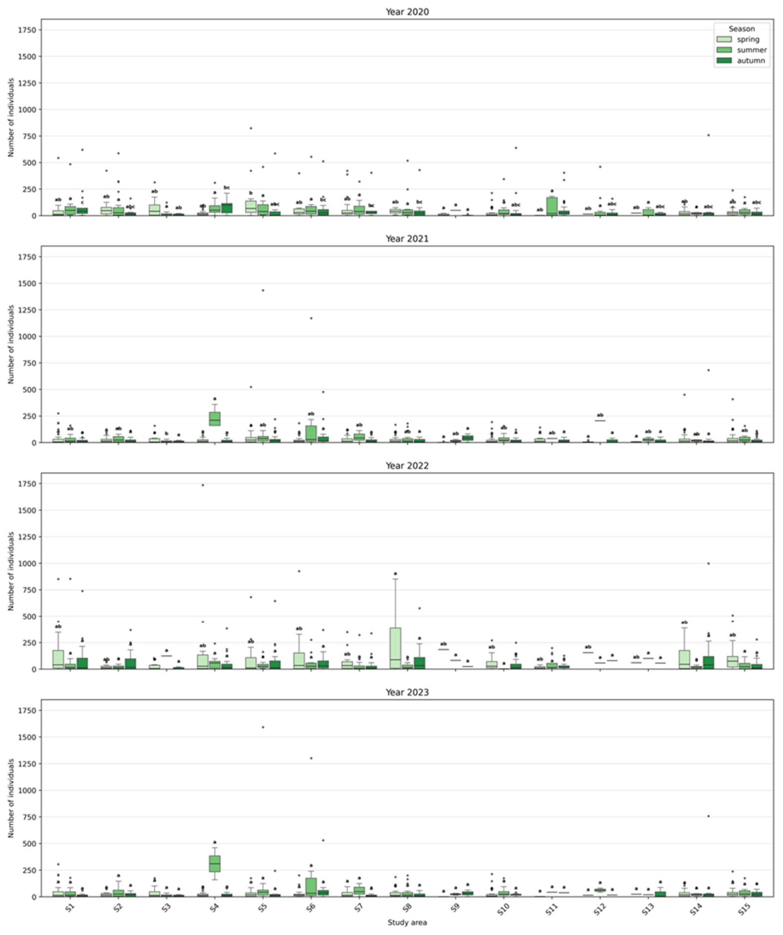
The Shapiro–Wilk analysis indicated that the dataset did not follow a normal distribution pattern (p = 1 × 10⁻⁵). The difference in the number of individuals between study areas (1–15), years, and seasons was tested by the Friedman test, which confirmed a significant difference (p = 0.016). The Kruskal–Wallis test confirmed significant differences in the number of individuals between study areas (1–15) (p = 0.001), seasonal periods (p = 0.001), and years (p = 0.002). The Mann–Whitney U test confirmed a significant difference (p = 0.018) in the number of individuals between management (without management and with management).

The results revealed pronounced spatial and temporal variability in the abundance of the monitored communities, with the implemented management measures playing a significant role. Study sites S1 and S4 served as control sites without management interventions, whereas restoration and management measures were implemented at S5–S15 throughout the entire monitoring period. Comparison of these two groups indicated that the managed sites generally exhibited greater variability in individual abundance, wider interquartile ranges, and a more frequent occurrence of extreme values. In contrast, the unmanaged control sites showed a more stable pattern of abundance, although consistently high abundance values were also recorded at site S4. From the perspective of seasonal dynamics, the lowest abundances were generally recorded in spring throughout all monitored years, whereas summer represented the period of the highest abundance at most study sites. During autumn, abundance generally declined again; however, at several managed sites, it remained higher than at the control sites, suggesting that favorable habitat conditions persisted beyond the main growing season. This trend was particularly evident at sites S6, S8, S14, and S15, where higher median abundances and greater variability were observed compared with the unmanaged control sites. Differences in the abundance of soil fauna were also evident among the monitored years. In 2020, abundance was relatively evenly distributed across the study sites, although elevated values were recorded particularly at S4 and S5. In 2021, a marked increase in abundance occurred at S4 during the summer season, whereas most other sites exhibited comparatively lower values. The highest interannual variability was observed in 2022, when several managed sites, especially S8 and S14, reached substantially higher abundance values and displayed broader variability. In 2023, high abundance was again confirmed at the unmanaged site S4; however, several managed sites (S6, S7, S14, and S15) also exhibited increased abundance, indicating that the effects of the implemented management measures persisted over time and contributed to maintaining abundant populations of soil fauna. Overall, the results indicate that management significantly influenced not only the mean abundance of individuals but also the spatial and temporal variability of soil fauna. While the unmanaged control sites (S1 and S4) provided relatively stable conditions with consistently high abundances, the managed sites (S5–S15) exhibited a more dynamic community structure and, in many cases, achieved higher abundance values, particularly during the summer season and in the final years of monitoring. These findings suggest that the implemented management measures promoted habitat restoration and created more favorable conditions for the development and persistence of soil fauna communities (Figure 2).

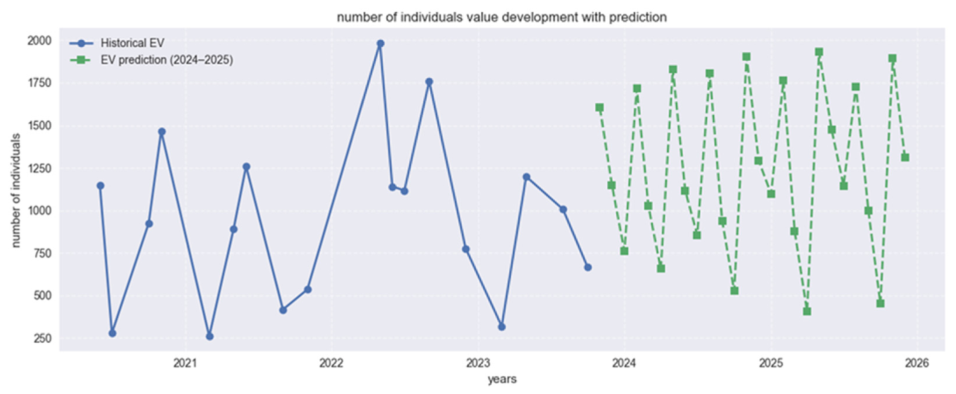
Long Short-Term Memory (LSTM) had the resulting MAPE value reach only 6.51%, demonstrating high predictive accuracy and excellent model performance.

The development of individual abundance in the forest habitats where management interventions were implemented showed considerable temporal fluctuations during the study period (Figure 3). Data from 2020–2023 indicate variations in abundance without a clear long-term increasing or decreasing trend. Throughout the monitoring period, phases of higher and lower abundance alternated, with the highest values recorded in 2022 and in the middle of 2023. In contrast, substantial declines in the number of individuals were also observed toward the end of the monitoring period. These decreases may be related to the natural dynamics of populations, seasonal changes in environmental conditions, or the ecosystem’s response to the implemented management interventions.

The predictive model suggests that the number of individuals will continue to exhibit considerable variability until the end of 2025. Predicted values range widely, from very low to high abundances, with recurring peaks exceeding 5000 individuals. This pattern indicates that the population is likely to maintain its dynamic character in the coming years. At the same time, the model does not predict a long-term decline in abundance but rather the continuation of cyclical fluctuations accompanied by the repeated occurrence of high abundance values. Therefore, the predicted results suggest that the implemented management measures create conditions that support the maintenance of relatively high individual abundance in forest habitats, although population dynamics remain highly variable over time.

The primary objective of the LSTM analysis was not merely to generate abundance forecasts but to evaluate whether management interventions contribute to maintaining long-term community stability. The predicted cyclic fluctuations without a persistent declining trend indicate that managed habitats retain suitable environmental conditions capable of supporting stable arthropod populations. Therefore, LSTM complements conventional statistical analyses by providing insight into the potential future trajectory of community development under current management practices.

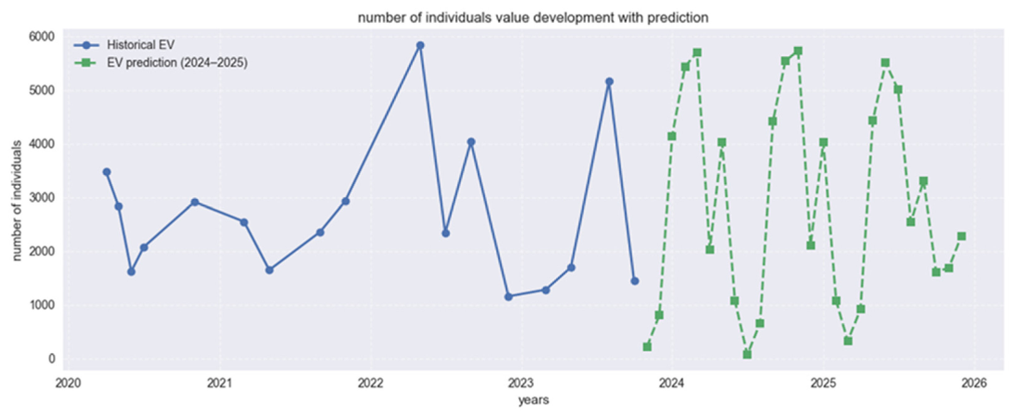
Long Short-Term Memory (LSTM) obtained an MAPE value of 12.6%, which indicates a high level of prediction accuracy and confirms the reliability of the developed model.

The development of individual abundance in open-area habitats where management interventions were implemented exhibited considerable interannual and seasonal variability during the monitoring period (Figure 4). Data from 2020–2023 indicate fluctuations in the abundance of individuals. The highest values were recorded during 2022 and 2023, whereas substantial declines in abundance occurred during certain periods. This pattern may reflect natural changes in species population dynamics, differences in habitat quality throughout the growing season, as well as the gradual effects of the implemented management interventions.

In the prediction until the end of 2025, despite the persistent variability, most predicted values are at levels comparable to or higher than the historical average, indicating the maintenance of suitable conditions for the occurrence of soil fauna. The modeling results further suggest that the management measures implemented in open habitats may contribute to maintaining a stable population, although individual abundance is expected to continue being influenced by the natural fluctuations characteristic of these dynamic ecosystems.

Measures such as mowing, controlled flooding, grazing, or restoration of hydrological connectivity modify vegetation complexity, litter accumulation, soil moisture, and microclimatic conditions. These environmental changes directly influence food availability, shelter, and breeding sites for ground-dwelling arthropods, thereby affecting both their abundance and community composition. Consequently, the temporal dynamics predicted by the LSTM model probably reflect not only natural population fluctuations but also the ecological response of arthropod communities to habitat management.

4. Discussion

The results of this study support Hypothesis 1, confirming that habitat type and management practices significantly affect the abundance, diversity, and community composition of soil fauna. The highest abundance was recorded in the unmanaged habitats (pasture and in the willow–poplar floodplain forest), suggesting that stable and not disturbed habitats provide more suitable conditions for the occurrence of soil fauna. Similar findings were reported by [17], who demonstrated that stable habitats support higher diversity and abundance of soil fauna compared to intensively managed areas. Floodplain forests are characterized by high litter production, favorable soil moisture, and a complex vegetation structure, all of which create suitable conditions for the development of numerous populations of soil fauna [18].

The dominance of the taxa Collembola, Coleoptera, and Isopoda observed in our study is consistent with the findings of several authors who identify these taxa as key components of soil and soil fauna ecosystems [19]. Collembola represent important decomposers involved in the breakdown of organic matter and the regulation of microbial activity in the soil, whereas Coleoptera and Isopoda significantly influence energy flow and nutrient cycling within the ecosystem [20].

The RDA analysis further supports Hypothesis 1 by demonstrating a clear differentiation of soil fauna communities between managed and unmanaged habitats. Most taxa were associated primarily with habitats without management interventions, suggesting their preference for more stable environmental conditions. These findings are consistent with those of [21,22,23], who reported that the natural dynamics of floodplain habitats create a wide range of microhabitats that support high invertebrate diversity. In contrast, more intensively managed areas exhibited greater heterogeneity in taxonomic composition, which may result from changes in vegetation structure, soil properties, and microclimatic conditions following the implementation of management measures.

The results of the multifactor ANOVA and One-way ANOVA support Hypothesis 2, showing that habitat management influences community stability and diversity. However, the response depends strongly on habitat type and management intensity. Similar findings have been reported by several studies focusing on soil fauna in wetland and floodplain ecosystems, where significant differences in abundance among habitats were observed due to variations in vegetation structure, soil moisture, and management intensity [24,25]. The highest abundances were recorded in willow–poplar floodplain forests and Pannonian poplar forests, which may be related to their greater structural vegetation diversity and more favorable microclimatic conditions. Forest habitats provide a larger amount of food resources, shelter, and more stable environmental conditions, thereby supporting higher abundance and diversity of invertebrates [26].

At the same time, pronounced seasonal fluctuations were recorded in these habitats, particularly during spring and summer, when biological activity and reproduction of many taxa increase. The significant influence of seasonality on organism abundance has also been confirmed in previous studies. Refs. [27,28] reported that the abundance of soil fauna varies according to seasonal changes in temperature, precipitation, and food availability, with the highest values typically recorded during the growing season. A similar trend was observed in the present study, where most habitats exhibited the highest abundances during spring and summer. Different population responses to applied management interventions were observed in managed habitats. The poplar nursery habitat showed high abundances, particularly during the summer, which may be related to regular mowing and subsequent vegetation regeneration. Similar results were reported by [29], who observed an increase in the abundance of soil fauna following restoration measures and the management of floodplain forests in the Danube floodplain area. Management practices may create a more heterogeneous environment and increase resource availability for many groups of invertebrates. In contrast, the lowest abundances were recorded in the pasture and alluvial meadow habitats. The lower abundance may be a consequence of reduced vegetation complexity, greater exposure to climatic factors, and lower availability of shelters. The relationship between vegetation diversity and the abundance of soil fauna has been repeatedly confirmed, with species-rich and structurally complex habitats supporting higher abundances of soil fauna. The hydrological regime also plays a crucial role in floodplain ecosystems. Seasonal flooding and fluctuations in groundwater levels represent key factors shaping invertebrate communities. Ref. [30] demonstrated that the flood pulse significantly influences the structure of insect communities in floodplain forests. These findings are also supported by the results of the present study, where pronounced seasonal differences were recorded primarily in floodplain forest habitats.

The predictive modeling supports Hypothesis 3 by indicating that, despite considerable temporal fluctuations, no long-term decline in soil fauna populations is expected under the current management regime. This trend may indicate a positive effect of the implemented management measures, which likely contribute to maintaining suitable conditions for the occurrence of the monitored soil fauna. Similar conclusions have been reported in several studies on ecosystem restoration, according to which restoration interventions can promote ecological stability and enhance the resilience of populations to environmental changes [31]. The variability in the abundance of orders recorded in both of our habitat groups (without management and with management) is characteristic of dynamic ecosystems influenced by seasonal changes, climatic factors, and food resource availability. Therefore, fluctuations in abundance may instead reflect natural population dynamics [32,33,34,35]. The predicted maintenance of high abundance values until the end of 2025 suggests that the implemented management measures may create favorable conditions for the long-term survival and reproduction of the monitored groups of organisms.

5. Conclusions

The results of the study confirmed that habitat type and management significantly influence the abundance, diversity, taxonomic composition, and trophic structure of communities. The highest abundance and diversity were recorded in floodplain forests, whereas more intensively managed open habitats exhibited lower values. The RDA analysis further demonstrated that management affects the representation of individual functional groups, particularly predators and detritivores, thereby indirectly influencing ecological processes such as organic matter decomposition, nutrient cycling, and the biological regulation of populations. The results also showed that management intensity, together with habitat structure, litter accumulation, soil moisture, and the hydrological regime, is the main factor shaping the diversity and functional structure of communities. Managed floodplain forests maintained high diversity, whereas intensively managed open habitats exhibited a decline in diversity. The LSTM predictive models indicated that, despite natural interannual fluctuations, no long-term decline in community abundance is expected through 2025. The models suggest a positive long-term effect of the implemented management measures, which contribute to maintaining the stability of communities and their ecological functions. Based on the obtained results, the conservation of habitat heterogeneity, restoration of the natural hydrological regime, extensive grazing, mowing, and the retention of habitat patches with a sufficient litter layer are recommended. Such management practices can promote higher soil fauna diversity, preserve functional diversity, and enhance the long-term ecological stability of floodplain ecosystems.