Ecological Security Under the SPMOR Paradigm: Spatiotemporal Assessment of Fanjingshan Region (2002–2022)

Abstract

Ecological security is fundamental to achieving the United Nations Sustainable Development Goals (SDGs) and maintaining ecosystem stability in ecologically sensitive regions. Mountainous protected areas, where ecological fragility and human pressure coexist, require dynamic evaluation frameworks that go beyond static pattern description. This study proposes an extended SPMOR (State–Pressure–Modelling–Optimization–Response) framework to assess the spatiotemporal evolution of ecological security in the Fanjingshan Mountain Region, a UNESCO World Heritage Site in Southwest China. Multi-source environmental and socio-economic datasets were standardized, objectively weighted using the CRITIC method, and integrated to construct a grid-based Ecological Security Index (ESI) for 2002, 2007, 2012, 2017, and 2022. Spatial autocorrelation analysis with global and local Moran’s I was employed to identify clustering patterns and temporal shifts. Results show that the average ESI increased from 0.4983 in 2002 to a peak of 0.5238 in 2012, before declining to 0.4945 in 2022. Global Moran’s I remained consistently high, ranging from 0.6516 to 0.6862, indicating persistent spatial clustering of ecological security. Spatially, the region exhibited a stable core–periphery structure, with high-security zones concentrated in the core reserve and low-security clusters distributed along human activity corridors. These findings suggest the coexistence of ecological restoration effects and renewed development pressures in mountainous protected areas. The proposed SPMOR framework provides a structured and potentially applicable approach for ecological security evaluation and offers practical insights for sustainable management of mountainous protected regions.

1. Introduction

Ecological security is a cornerstone of global sustainability and an essential foundation for achieving the United Nations Sustainable Development Goals (SDGs), particularly SDG 13 (Climate Action), SDG 15 (Life on Land), and SDG 11 (Sustainable Cities and Communities) [1,2,3,4]. A secure and resilient ecological pattern ensures the maintenance of ecosystem services such as carbon sequestration, water regulation, and biodiversity conservation, which underpin sustainable human well-being and climate resilience [5]. However, accelerating land-use transitions and ecological degradation driven by urbanization and human disturbance have increasingly threatened regional ecological stability [6,7,8,9]. Understanding the spatial configuration and temporal evolution of ecological security has therefore become crucial for guiding spatial governance and ecological restoration strategies aligned with the SDG framework.

In China’s mountainous regions, rapid socio-economic development has reshaped land systems and intensified ecological vulnerability [10,11,12]. These pressures are especially pronounced in ecologically sensitive and protected areas, where complex terrain and human–environment interactions heighten the risk of fragmentation and degradation. The Fanjingshan Region—a UNESCO World Heritage Site and one of China’s most intact subtropical forest ecosystems [13]—provides vital services such as water regulation, soil conservation, and biodiversity maintenance to surrounding counties and cities. Yet, the spatiotemporal pattern and clustering dynamics of ecological security in Fanjingshan and its peripheral zones remain insufficiently understood, limiting the evidence base for coordinated conservation and regional development. A comprehensive spatiotemporal assessment is therefore needed to reveal the evolution of its ecological security pattern and to support sustainable management of world-class mountain parks.

Existing methods for assessing ecological security patterns have primarily relied on the Pressure–State–Response (PSR) framework, which has been widely applied to evaluate ecosystem health, environmental vulnerability, and land-use sustainability in various regions. For example, Zhou et al. applied the PSR model to assess ecological security in the Wuling Mountains, identifying the trade-offs between ecological protection and agricultural expansion [14]; Yu et al. evaluated the ecological pattern of the upper Yangtze River Basin using multi-source indicators of land cover, socio-economic pressure, and ecosystem service value [15]; and Sun et al. integrated PSR with spatial statistical models to analyze the ecological resilience of mountainous counties in Guizhou Province [16]. Beyond these Chinese case studies, international research has also applied ecological security or ecosystem-condition assessment frameworks to broader environmental contexts, including PSR-based watershed health assessment in central Iran and ecosystem-condition assessment across European rivers, lakes, and coastal waters [17,18]. These studies have demonstrated the explanatory power of the PSR framework in identifying key stressors and spatial gradients of ecological security. They demonstrate the PSR framework’s strength in identifying key stressors and spatial gradients of ecological security. Yet, PSR mainly links pressure, state, and response, offering limited insight into the broader causal chain of ecological change. DPSIR partially overcomes this by adding driving forces and impacts, enhancing understanding of human–environment interactions. However, DPSIR applications in ecological security assessments often remain focused on causal diagnosis, with insufficient attention to temporal ecological evolution and the translation of findings into spatially targeted governance priorities. Thus, an integrated framework—linking ecological status diagnosis, pressure identification, temporal evolution assessment, spatial priority mapping, and management response—is still needed for mountainous protected areas.

To address these limitations, this study proposes an integrated SPMOR paradigm (State–Pressure–Modelling–Optimization–Response) for ecological security evaluation, aiming to connect ecological status diagnosis, pressure identification, temporal evolution assessment, spatial priority recognition, and management response within a unified framework. Specifically, the State, Pressure, and Response layers follow the conventional PSR logic, while the added Modelling and Optimization layers complement PSR- and DPSIR-based assessments by incorporating retrospective temporal indicators and land-use regulation indicators. The Modelling layer characterizes ecological evolution, vegetation change, and potential degradation risks, whereas the Optimization layer is operationalized as an optimization-oriented diagnostic component that evaluates ecological land allocation rationality and high-intensity land-use pressure. Taking the Fanjingshan National Nature Reserve as a case study, this research integrates multi-source environmental and socio-economic data from 2002 to 2022 to construct an Ecological Security Index (ESI), analyze its spatiotemporal evolution and spatial clustering characteristics, and provide scientific support for ecological restoration prioritization and land-use regulation in mountainous protected areas.

2. Study Area and Data

2.1. Study Area

The Fanjingshan Region, located in Tongren City, Guizhou Province, Southwest China (Figure 1), lies within the core area of the Wuling Mountains and serves as one of the most representative subtropical forest ecosystems in East Asia. The region is characterized by steep terrain, large elevation gradients (388–2444 m), and highly heterogeneous ecological landscapes, encompassing forest, shrub, grassland, and cultivated land mosaics. Designated as a UNESCO World Natural Heritage Site and National Nature Reserve, Fanjingshan plays a critical role in biodiversity conservation, water regulation, and soil erosion control, functioning as an ecological barrier for the upper reaches of the Yangtze River [19].

This region was selected as a case study for three main reasons. First, Fanjingshan represents a typical mountainous protected area where ecological sensitivity and human pressures coexist—making it ideal for testing dynamic ecological security frameworks. Second, its well-documented land-use transformations and ecological restoration efforts over the past two decades provide a solid empirical basis for long-term spatiotemporal analysis. Third, as a world-class ecological conservation area surrounded by rapidly developing counties and towns, Fanjingshan exemplifies the broader challenge of coordinating conservation and development in mountainous regions of China. Therefore, analyzing its spatiotemporal ecological security pattern not only deepens our understanding of the mechanisms shaping mountain ecosystem resilience but also provides transferable insights for the sustainable management of similar protected landscapes worldwide.

2.2. Data

This study integrates multi-source environmental and socio-economic datasets to construct an ecological security evaluation framework for the Fanjingshan Region (

Table 1. Data source.

Data Name	Resolution	Year	Data Source
Land Surface Temperature (LST)	1 km × 1 km	2002, 2007, 2012, 2017, 2022	MODIS/Terra Land Surface Temperature/Emissivity Daily L3 Global 1 km SIN Grid V061 [20]
Evapotranspiration (ET)	500 m × 500 m	2002, 2007, 2012, 2017, 2022	MODIS/Terra Net Evapotranspiration Gap-Filled 8-Day L4 Global 500 m SIN Grid V061 [21]
Land use	30 m × 30 m	2002, 2007, 2012, 2017, 2022	30 m annual land cover dataset of China from 1985 to 2023 [22]
Digital Elevation Model (DEM)	30 m × 30 m	/	SRTM DEM Version 4.1 [23]
Population Density (PopDen)	1 km × 1 km	2002, 2007, 2012, 2017, 2020	WorldPop individual countries 1 km population density dataset [24]
Fractional Vegetation Cover (FVC)	250 m × 250 m	2002, 2007, 2012, 2017, 2022	China regional 250 m fractional vegetation cover dataset (2000–2023) [25]
Gross Domestic Product (GDP)	1 km × 1 km	2002, 2007, 2012, 2017, 2020	China GDP spatial distribution kilometer grid dataset [26]
Net Primary Productivity (NPP)	500 m × 500 m	2002, 2007, 2012, 2017, 2022	MODIS/Terra Net Primary Production Gap-Filled Yearly L4 Global 500 m SIN Grid V061 [27]
District Boundary	/	2024	Standard map service/official boundary dataset, No. GS(2024)0650

Note: 2022 assessment used the 2020 PopDen/GDP dataset as a proxy due to data availability.

). The datasets include remotely sensed and statistical indicators representing land surface temperature (LST), evapotranspiration (ET), land use, digital elevation model (DEM), population density (PopDen), fractional vegetation cover (FVC), gross domestic product (GDP), and net primary productivity (NPP). The temporal coverage spans 2002, 2007, 2012, 2017, and 2022, corresponding to five representative periods of ecological and socio-economic change in the study area (for the 2022 assessment, the 2020 PopDen and GDP datasets were used due to data availability limitations). All spatial datasets were projected to the CGCS 2000/Gauss–Krüger Zone 39N (EPSG: 4547) coordinate system and resampled to a 1 km × 1 km spatial resolution to ensure spatial consistency and comparability among variables. The 1 km resolution was adopted to accommodate the relatively low-resolution datasets used in this study, and it provides an appropriate balance between data consistency and ecological security risk assessment at the regional scale. All data used in this research are derived from publicly available and authoritative sources, including NASA LP DAAC (MODIS products), SRTM DEM Version 4.1, the Resource and Environment Data Cloud Platform (RESDC), and regional datasets published by the National Earth System Science Data Center.

3. Methodology

This study follows a structured methodological workflow grounded in the SPMOR paradigm (Figure 2). First, an indicator system is developed and hierarchically organized into five layers—State, Pressure, Modelling, Optimization, and Response—to capture the full spectrum of ecological security dynamics. Second, all indicators are normalized using the range standardization method, and objective weights are derived through the CRITIC approach, which accounts for both variability and inter-indicator correlation. Third, a grid-based Ecological Security Index (ESI) is constructed through weighted linear aggregation of the standardized indicators. Finally, spatiotemporal patterns of ecological security from 2002 to 2022 are examined using global and local Moran’s I, providing insight into spatial clustering, local anomalies, and governance priorities.

3.1. SPMOR Model

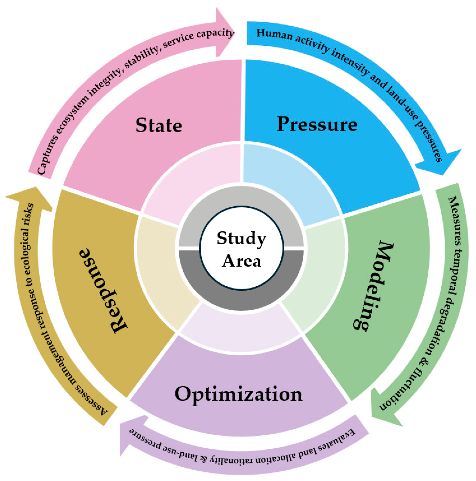
The SPMOR framework consists of five layers: State, Pressure, Modelling, Optimization, and Response (Figure 3). Indicator assignment was based on the primary ecological diagnostic function of each variable, following the conceptual logic of the PSR framework and its extended applications in ecological security assessment [28].

The State layer describes the current ecological condition and ecosystem service capacity, including land surface temperature, evapotranspiration, landscape pattern metrics, and ecosystem service value.

The Pressure layer reflects external disturbances and human activity intensity through indicators such as population density, steep-slope cultivated land, regional development intensity, land-use intensity, and distance to construction land.

The Response layer reflects the capacity of socio-ecological systems to cope with pressures and support ecological recovery [28,29]. Based on this interpretation, GDP per unit area, ecosystem resilience, and distance to the core ecological zone were selected to characterize socio-economic support capacity, natural recovery potential, and the spatial governance context, respectively.

The Modelling layer is interpreted as a modelling-oriented diagnostic component that integrates indicators derived from ecological assessment models and temporal change analyses to characterize ecological vulnerability, sensitivity, and historical ecosystem dynamics, rather than to simulate or predict future conditions. Specifically, the slope–FVC vulnerability index represents ecological vulnerability associated with terrain and vegetation conditions, while NDVI change trends and land-use change frequency characterize vegetation dynamics and land-use transitions over time.

The Optimization layer evaluates the potential for ecological restoration and land-use regulation. Ecological land allocation rationality reflects the adequacy of ecological land within each grid, whereas high-intensity land-use pressure identifies areas requiring stricter development control or ecological restoration.

All indicators were standardized and assigned to a single SPMOR layer (

Table 2. Ecological security evaluation index system of the Fanjingshan Region.

Target Layer	Criterion Layer	Index Layer	Code	Unit	Direction
Ecological Security Index for the Fanjingshan Region	State	Land surface temperature	X1	°C	−
		Evapotranspiration (ET)	X2	mm	−
		Patch Density (PD)	X3	patches/km2	−
		Patch Cohesion Index (COHESION)	X4	%	+
		Shannon Diversity Index (SHDI)	X5	dimensionless	+
		Shannon Evenness Index (SHEI)	X6	dimensionless	+
		Ecosystem Service Value (ESV)	X7	Yuan	+
	Pressure	Population Density	X8	persons/km2	−
		Percentage of cultivated area on steep slopes	X9	%	−
		Regional Development Index	X10	%	−
		Land Use Intensity	X11	%	−
		Distance to Construction Land	X12	Km	−
	Modelling	Slope–FVC Vulnerability Index	X13	dimensionless	−
		NDVI Change Trend Index	X14	yr−1	+
		Land Use Change Frequency	X15	times	−
	Optimization	Ecological Land Allocation Rationality	X16	dimensionless	+
		High-Intensity Land-Use Pressure	X17	%	−
	Response	GDP per unit area	X18	Yuan/km2	+
		Ecosystem Resilience	X19	dimensionless	+
		Distance to Core Ecological Zone	X20	Km	+

). A consistent sign convention was adopted, where “+” indicates a positive contribution to ecological security, and “−“ indicates a negative contribution.

(1) State: This layer characterizes baseline ecosystem condition—structural integrity, functional stability, and service capacity—via landscape configuration and composition metrics and service valuation. X1 Land Surface Temperature (LST, −) captures thermal stress and surface energy balance as a first-order proxy of ecosystem condition. X2 Evapotranspiration (ET, −) reflects land–atmosphere water exchange through soil evaporation and vegetation transpiration. In this study, higher ET indicates greater water consumption and potential water loss, which may reduce soil moisture and available water resources. Therefore, from the perspective of water conservation and ecological security, ET was treated as a negative indicator in the ESI calculation [30,31]. Landscape structure is then characterized by X3 Patch Density (PD, −) and X4 Patch Cohesion Index (COHESION, +) following FRAGSTATS conventions: PD quantifies fragmentation intensity (Equation (1)), while COHESION measures physical connectedness of class i (Equation (2)) [32]. Compositional heterogeneity is captured by X5 Shannon Diversity Index (SHDI, +) and X6 Shannon Evenness Index (SHEI, +), computed by Equations (3) and (4), which diagnose richness and balance of land-cover types at the landscape scale. Finally, service provision capacity is monetized by X7 Ecosystem Service Value (ESV, +) using the equivalent-factor method localized for Fanjingshan (Equation (5)); this approach is widely adopted in regional studies because it is transparent and requires relatively few input parameters [33]. The local standard equivalent value was then multiplied by the ecosystem service equivalent coefficients assigned to each land-use category and converted to yuan/km². The resulting category-specific ESV coefficients are reported in

Table 3. Table of ecosystem service value coefficients for each category (unit: yuan/km²).

	Cropland	Forest	Grassland	Water	Shrub
ESV coefficient	308,895.34	1,540,371.12	1,216,813.03	9,822,871.78	1,345,870.55

.

$$\mathrm{P}\mathrm{D}={\displaystyle \frac{N}{A_{{\mathrm{k}\mathrm{m}}^2}}}\left(\mathrm{patches}{\mathrm{k}\mathrm{m}}^{-2}\right)$$

(1)

$${\mathrm{C}\mathrm{O}\mathrm{H}\mathrm{E}\mathrm{S}\mathrm{I}\mathrm{O}\mathrm{N}}_i={\displaystyle \frac{\left[1-\frac{{\displaystyle {\sum }_{j=1}^{n_i}}{p}_{ij}}{{\displaystyle {\sum }_{j=1}^{n_i}}{p}_{ij}\sqrt{a_{ij}}}\right]}{\left(1-\frac{1}{\sqrt{A}}\right)}}\times 100$$

(2)

where $N$ is the total patch count, $A_{{\mathrm{k}\mathrm{m}}^2}$ the landscape area (${\mathrm{k}\mathrm{m}}^2$), $p_{ij}$ and $a_{ij}$ the perimeter and area of the $j$-th patch of class $i$, and $A$ the landscape area in cell units.

$$\mathrm{S}\mathrm{H}\mathrm{D}\mathrm{I}=-{\displaystyle \sum _{k=1}^m}{p}_k\ln p_k$$

(3)

$$\mathrm{S}\mathrm{H}\mathrm{E}\mathrm{I}={\displaystyle \frac{\mathrm{S}\mathrm{H}\mathrm{D}\mathrm{I}}{\ln m}}$$

(4)

with $p_k$ being the area share of class $k$ and $m$ the number of classes.

$$ESV={\displaystyle \sum _{i=1}^m}{\displaystyle \sum _{j=1}^n}{S}_{ij}\cdot P_{ij}$$

(5)

where $S_{ij}$ (yuan ${\mathrm{k}\mathrm{m}}^{-2}$) is the unit-area value coefficient of service $j$ for land-use type $i$, and $P_{ij}$ is the corresponding area.

(2) Pressure: This layer identifies external stressors with emphasis on human-activity intensity and land-use disturbance. X8 Population Density (−) represents human activity intensity and background anthropogenic pressure [34]. X9 Percentage of cultivated area on steep slopes (−) flags erosion-prone farming where slope > 15°, computed by Equation (6), consistent with soil-loss/erosion standards (RUSLE/CSLE) [35]. X10 Regional Development Index, RDI (−), aggregates cropland and construction-land shares via Equation (7) to provide a compact proxy of urbanization intensity and the human footprint [36]. X11 Land-Use Intensity (−) was calculated as the area-weighted sum of land-use intensity grades across land-use classes (Equation (8)), reflecting the overall intensity of human land utilization within each grid [37]. X12 Distance to Construction Land (+)—the Euclidean distance to the nearest built-up pixel—captures edge-driven disturbance and encroachment pressure recognized in landscape ecology edge-effect theory.

$$\mathrm{\%}\mathrm{Steep}\mathrm{Cropland}={\displaystyle \frac{A_{\mathrm{crop},\mathrm{slope}>{15}^{\circ }}}{A_{\mathrm{cell}}}}\times 100$$

(6)

$$\mathrm{R}\mathrm{D}\mathrm{I}={\displaystyle \frac{F+C}{\mathrm{T}\mathrm{A}}}$$

(7)

where $F$ is the cropland area, $C$ is the construction-land area, and TA is the cell area.

$$L={\displaystyle \sum _{i=1}^n}\left(C_i{P}_i\right)$$

(8)

where $C_i$ is the land-use intensity grade of land-use class $i$, and $P_i$ is the area proportion of land-use class (i) within the grid.

(3) Modelling: This layer expresses temporal evolution to anticipate system trajectories. X13 Slope–FVC Vulnerability Index (−) (Equation (9)) couples topographic sensitivity with vegetation stability, following ecological vulnerability assessment practice in erosion-prone regions [38]. A higher value indicates a greater risk of degradation under disturbance. The X14 NDVI Change Trend Index (+) (Equation (10)) is calculated separately for each assessment interval (e.g., 2000–2005, 2005–2010, etc.) by performing a pixel-wise linear regression of annual NDVI values within that interval, and the resulting slope is used to represent the direction and magnitude of vegetation change during that specific period, which is widely used to indicate vegetation degradation or recovery in remote-sensing ecology [39]. X15 Land-Use Change Frequency (−) (Equation (11)) is also computed for each assessment interval by counting the number of land-use type transitions for each pixel between consecutive land-cover maps within that interval (e.g., changes from 2000 to 2005, 2005 to 2010, etc.), thereby quantifying the frequency of land-use conversions during that period as a proxy for disturbance intensity and spatial instability in land-system science [40].

$$\mathrm{V}\mathrm{u}\mathrm{l}=S^{*}\left(1-V^{*}\right)$$

(9)

where $S^{\mathrm{*}}$ is the normalized slope, and $V^{\mathrm{*}}$ is the normalized fractional vegetation cover (FVC).

$$\beta ={\displaystyle \frac{n\sum t{\mathrm{N}\mathrm{D}\mathrm{V}\mathrm{I}}_t-\left(\sum t\right)\left(\sum {\mathrm{N}\mathrm{D}\mathrm{V}\mathrm{I}}_t\right)}{n\sum t^2-{\left(\sum t\right)}^2}}$$

(10)

where $\beta$ is the regression slope of the NDVI time series for each pixel within the corresponding assessment interval.

$$\mathrm{L}\mathrm{C}{\mathrm{F}}_j={\displaystyle \sum _{k=1}^{m_j-1}}I\left({\mathrm{class}}_{j,k}\ne {\mathrm{class}}_{j,k+1}\right)$$

(11)

where ${\mathrm{L}\mathrm{C}\mathrm{F}}_j$ is the land-use change frequency within assessment interval $j$, ${\mathrm{class}}_{j,k}$ is the land-use class at time $k$ within interval $j$, $m_j$ is the number of land-use observations in that interval, and I(·) equals 1 when a land-use transition occurs and 0 otherwise.

(4) Optimization: This layer is operationalized as an optimization-oriented diagnostic component that evaluates the rationality of ecological land allocation and high-intensity land-use pressure. X16 Ecological Land Allocation Rationality (ELAR, +) (Equation (12)) measures the proportion of ecological land (forest, grassland, and water bodies) within each grid cell, reflecting the adequacy and spatial support capacity of ecological land in maintaining ecosystem stability [15]. A higher RELA indicates a more favorable ecological land structure, consistent with conservation-planning theory emphasizing connectivity [41]. X17 Proportion of High-Intensity Land Use (PHILU, −) (Equation (13)) quantifies the share of impervious or construction land, capturing the encroachment effect of intensive human activities and serving as a negative optimization indicator [42].

$$\mathrm{ELAR}={\displaystyle \frac{A_{\mathrm{forest}}+A_{\mathrm{grass}}+A_{\mathrm{water}}}{A_{\mathrm{cell}}}}$$

(12)

where $A_{\mathrm{forest}},A_{\mathrm{grass}}$, and $A_{\mathrm{water}}$ are the areas of forest, grassland, and water bodies within the grid cell, and $A_{\mathrm{cell}}$ is the total cell area.

$$\mathrm{P}\mathrm{H}\mathrm{I}\mathrm{L}\mathrm{U}={\displaystyle \frac{A_{\mathrm{impervious}}}{A_{\mathrm{cell}}}}$$

(13)

where $A_{\mathrm{impervious}}$ is the area of high-intensity land use (impervious/construction land) within the grid cell, and $A_{\mathrm{cell}}$ is the total cell area.

(5) Response: This layer evaluates the management capacity and societal response to ecological risks, serving as the institutional guarantee for ecological restoration and sustainable management. X18 GDP per unit area (+) was used to represent regional socio-economic support capacity within the Response layer. Therefore, GDP per unit area was treated as a positive indicator in the ESI calculation, while development-related pressures were represented separately by indicators such as regional development intensity, land-use intensity, and high-intensity land-use pressure [43]. X19 Ecosystem Resilience (NPP, +) measures the capacity of ecosystems to maintain and recover functions after disturbance, with net primary productivity widely recognized as a robust proxy for resilience [44]. X20 Distance to Core Ecological Zone (+) captures the spatial proximity to strictly protected areas, reflecting the effectiveness of zoning policies in mitigating human disturbance and providing refuge for biodiversity [45].

3.2. CRITIC Objective Weight Analysis

To ensure the comparability of indicators with different units and magnitudes, all raw data were first normalized using the range standardization method. For positive indicators, where larger values indicate higher ecological security, normalization follows Equation (14). For negative indicators, where larger values denote stronger stress or lower security, normalization follows Equation (15). This step eliminates the influence of scale heterogeneity and enables the integration of diverse ecological, environmental, and socioeconomic variables into a unified evaluation framework [46].

$$x_{ij}^{\prime }={\displaystyle \frac{x_{ij}-x_j^{min}}{x_j^{max}-x_j^{min}}}$$

(14)

$$x_{ij}^{\prime }={\displaystyle \frac{x_j^{max}-x_{ij}}{x_j^{max}-x_j^{min}}}$$

(15)

where $x_{ij}^{\prime }$ is the raw value of indicator $j$ for grid cell $i$, $x_{ij}^{\prime }$ is the normalized value, and $x_j^{max}$ and $x_j^{min}$ are the maximum and minimum values of indicator $j$ across all grid cells, respectively.

Following normalization, the CRITIC method (Criteria Importance Through Intercriteria Correlation) was applied to determine indicator weights objectively. Unlike subjective weighting approaches such as AHP, CRITIC accounts for both the contrast intensity of each indicator (standard deviation) and its conflict with others (correlation), thereby providing a robust and data-driven weighting scheme [47]. Specifically, the information content of indicator j is calculated as in Equation (16).

$$C_j={\sigma }_j{\displaystyle \sum _{k=1}^p}\left(1-r_{jk}\right)$$

(16)

where ${\sigma }_j$ is the standard deviation of indicator $j$, and $r_{jk}$ is the Pearson correlation coefficient between indicators $j$ and $k$. The normalized weight is then given by Equation (17).

$$w_j={\displaystyle \frac{C_j}{{\displaystyle {\sum }_{m=1}^p}{C}_m}},{\displaystyle \sum _{j=1}^p}{w}_j=1$$

(17)

To assess the robustness of the ESI results to the weighting scheme, a sensitivity analysis was performed by perturbing the CRITIC-derived weights. For each year, weights were randomly varied within ±10% and then normalized to sum to 1. This process was repeated 1000 times, with ESI recalculated each time. Robustness was evaluated using the mean ESI, standard deviation, coefficient of variation, and Spearman’s rank correlation with the baseline results.

3.3. Ecological Security Index (ESI) Spatiotemporal Analysis

After indicator construction (Section 3.1) and objective weighting via CRITIC (Section 3.2), we synthesized a cell-level Ecological Security Index (ESI) by linearly aggregating the standardized indicators $z_{ijt}$ with the weight vector $w_j$. For grid cell $i$ in year $t$, the ESI is given by Equation (18).

$${\mathrm{E}\mathrm{S}\mathrm{I}}_{it}={\displaystyle \sum _{j=1}^p}{w}_j{z}_{ijt},{\displaystyle \sum _{j=1}^p}{w}_j=1$$

(18)

Spatiotemporal patterns are then assessed with Moran’s statistics [48]. Global Moran’s I (overall spatial dependence) is given by Equation (19).

$$I_t={\displaystyle \frac{n}{S_0}}{\displaystyle \frac{\sum _i\sum _j{w}_{ij}\left({\mathrm{E}\mathrm{S}\mathrm{I}}_{it}-{\overline{E}}_t\right)\left({\mathrm{E}\mathrm{S}\mathrm{I}}_{jt}-{\overline{E}}_t\right)}{\sum _i{\left({\mathrm{E}\mathrm{S}\mathrm{I}}_{it}-{\overline{E}}_t\right)}^2}},$$

(19)

And local Moran’s I (LISA) (local clusters/outliers) is given by Equation (20).

$$I_{i,t}={\displaystyle \frac{\left({\mathrm{E}\mathrm{S}\mathrm{I}}_{it}-{\overline{E}}_t\right)}{m_{2,t}}}\sum _j{w}_{ij}\left({\mathrm{E}\mathrm{S}\mathrm{I}}_{jt}-{\overline{E}}_t\right),m_{2,t}={\displaystyle \frac{1}{n}}\sum _i{\left({\mathrm{E}\mathrm{S}\mathrm{I}}_{it}-{\overline{E}}_t\right)}^2.$$

(20)

Here, $n$ is the number of cells; ${\bar{E}}_t$ is the mean ESI at time $t;w_{ij}$ are row-standardized spatial weights (queen contiguity); $S_0=\sum _i\sum _j{w}_{ij}$. Positive $I_t$ indicates clustering; values near zero imply randomness. Significance for $I_t$ and $I_{i,t}$ was evaluated using 999 random permutations. The significance threshold was set at (p < 0.05). For LISA analysis, false discovery rate (FDR) correction was applied to local Moran’s I p-values to reduce the potential inflation of Type I error caused by multiple local tests. Only grid cells that remained significant after FDR correction were classified as HH, LL, HL, or LH clusters/outliers in the LISA maps; otherwise, they were treated as not significant.

4. Results

4.1. ESI Construction Result Based on SPMOR

The Ecological Security Index (ESI) of the Fanjingshan Region was constructed based on the standardized multi-indicator system under the SPMOR framework, with objective weights derived from the CRITIC method (

Table 4. Temporal evolution of ESI indicator weights based on the CRITIC method (2002–2022).

Criterion Layer	Index	2002	2007	2012	2017	2022
State	X1	0.0578	0.0633	0.0638	0.0628	0.0604
	X2	0.0614	0.0608	0.0575	0.0676	0.0703
	X3	0.0504	0.0533	0.0397	0.0399	0.0443
	X4	0.0057	0.0055	0.0053	0.0053	0.0051
	X5	0.1271	0.1133	0.1270	0.1291	0.1258
	X6	0.1380	0.1258	0.1191	0.1211	0.1209
	X7	0.0284	0.0295	0.0300	0.0223	0.0220
Pressure	X8	0.0324	0.0405	0.0251	0.0247	0.0244
	X9	0.0151	0.0169	0.0193	0.0178	0.0194
	X10	0.0407	0.0424	0.0430	0.0418	0.0421
	X11	0.0346	0.0342	0.0378	0.0338	0.0337
	X12	0.0759	0.0815	0.0868	0.0850	0.0894
Modelling	X13	0.0443	0.0354	0.0423	0.0400	0.0213
	X14	0.0233	0.0321	0.0277	0.0228	0.0210
	X15	0.0414	0.0504	0.0542	0.0485	0.0466
Optimization	X16	0.0369	0.0380	0.0387	0.0377	0.0376
	X17	0.0119	0.0129	0.0170	0.0199	0.0222
Response	X18	0.0330	0.0311	0.0259	0.0275	0.0290
	X19	0.0429	0.0429	0.0463	0.0576	0.0701
	X20	0.0987	0.0904	0.0935	0.0949	0.0944

). The temporal evolution of indicator weights reflects shifting contributions of ecological, anthropogenic, and management-related factors to regional security. Notably, indicators such as land surface temperature (X1), landscape diversity (X5–X6), and distance to construction land (X12) consistently exhibited relatively high weights, suggesting that both landscape structure and development pressure remain key determinants of ecological security in mountainous contexts. Similar patterns have been identified in other studies on ecologically fragile zones, where spatial fragmentation and edge effects significantly influence ecosystem vulnerability [12,14].

Based on the ESI grading criteria (

Table 5. Security level classification criteria for the Ecological Security Index (ESI).

Level	Type	Index Range	Description of Security Level Characteristics
I	Very Low Security	[0.35, 0.40)	Highly fragmented and disturbed; low resilience; urgent restoration needed.
II	Low Security	[0.40, 0.45)	Unstable pattern; vulnerable to external stress; low resilience.
III	Critical Security	[0.45, 0.50)	Near tipping point; prone to sudden degradation under pressure.
IV	Moderate Security	[0.50, 0.55)	Moderately stable; some self-regulation; resilience improving.
V	High Security	[0.55, 0.60)	Good structure and function; strong service provision and coordination.
VI	Very High Security	[0.60, 0.70]	Highly resilient and organized; excellent connectivity and resistance.

Note: The classification thresholds were defined by the equal-interval method for relative comparison within the Fanjingshan Region.

), the spatiotemporal distribution of ecological security was visualized at five time points (Figure 4). Overall, the region exhibits a patchy and gradient-like pattern, with higher-security areas concentrated in the core protected zones in the north and south, while the central corridor, which is more affected by human activity and infrastructure, displays relatively lower security. Between 2002 and 2012, the spatial extent of moderate-security areas increased steadily, indicating improvements in landscape stability and ecological resilience. This pattern is broadly consistent with previous studies showing that large-scale ecological restoration programs in China, such as the Natural Forest Protection Program (NFPP) and Grain-for-Green policies, have contributed to vegetation recovery and ecosystem improvement [49]. However, the distributions in 2017 and 2022 show a subtle re-expansion of lower-security zones, particularly in the central and eastern foothill areas, suggesting renewed disturbance or pressure that may be associated with land-use intensification and tourism-related development in peripheral zones.

The annual average ESI values further corroborate the temporal pattern of ecological security in the Fanjingshan Mountain Region (

Table 6. Annual average Ecological Security Index (ESI) and corresponding security levels in the Fanjingshan Region (2002–2022).

Year	Ave ESI	Level	Type
2002	0.4983	III	Critical
2007	0.5131	IV	Moderate
2012	0.5238	IV	Moderate
2017	0.5009	IV	Moderate
2022	0.4945	III	Critical

). From a critical level of 0.4983 in 2002 (Level III), the index steadily increased to moderate security (Level IV) between 2007 and 2017, peaking at 0.5238 in 2012. This upward trend reflects the cumulative effects of national ecological restoration projects implemented during the early 2000s—such as the Grain for Green Program and mountain reforestation initiatives—which enhanced vegetation cover and reduced surface fragmentation. However, the subsequent decline to 0.4945 in 2022 may indicate emerging ecological stress associated with intensified urban expansion, infrastructure construction, and tourism pressure in peripheral zones. The oscillating trajectory of ESI over two decades thus reveals a pattern of “restoration followed by re-disturbance,” a phenomenon similarly observed in other mountainous protected areas where ecological gains are vulnerable to renewed anthropogenic activity. Overall, the ESI framework effectively captures these fine-scale spatial heterogeneities and temporal inflections, demonstrating its robustness in diagnosing both ecological recovery and latent risks. These findings provide an empirical foundation for subsequent optimization and response strategies aimed at sustaining the long-term ecological resilience of world-class mountain parks.

To assess robustness, a sensitivity analysis was conducted by perturbing CRITIC-derived weights within ±10%. As shown in

Table 7. Sensitivity analysis of ESI results under ±10% perturbations of CRITIC-derived weights.

Year	Mean ESI Under Perturbation	SD	CV (%)	Spearman’s $\mathit{\rho }$
2002	0.4983	0.0013	0.25	0.9976
2007	0.5130	0.0012	0.23	0.9977
2012	0.5237	0.0013	0.24	0.9972
2017	0.5009	0.0012	0.24	0.9970
2022	0.4945	0.0012	0.23	0.9979

, the mean ESI values remained broadly consistent with the baseline results reported in Table 6, exhibiting low variability (SD: 0.0012–0.0013; CV: 0.23–0.25%) and high rank consistency (Spearman’s $\rho$: 0.9970–0.9979). These findings suggest that the ESI results are relatively stable under moderate changes in indicator weights.

4.2. Spatial Autocorrelation and Clustering Characteristics of ESI

To further examine the spatial dynamics of ecological security in the Fanjingshan Region, both global and local spatial autocorrelation analyses were conducted based on the Ecological Security Index (ESI). The results of global Moran’s I (

Table 8. Global spatial autocorrelation of the Ecological Security Index (ESI) in the Fanjingshan Region (2002–2022).

Year	Moran’s I	z-Score	p-Value	Type
2002	0.651640	55.005375	0.000000	Clustered
2007	0.644063	54.376364	0.000000	Clustered
2012	0.649694	54.834088	0.000000	Clustered
2017	0.683555	57.673416	0.000000	Clustered
2022	0.686220	57.724622	0.000000	Clustered

) indicate a consistently high level of spatial clustering throughout 2002–2022, with Moran’s I values ranging from 0.64 to 0.69 (p < 0.001). These statistically significant positive correlations suggest that areas with similar ecological security levels tend to be spatially aggregated, reflecting strong spatial dependence and stable ecological structures within the mountainous system. The Moran’s I values remained consistently high throughout the study period, with a slight increase from 0.6516 in 2002 to 0.6862 in 2022. This pattern suggests persistent spatial clustering of ecological security and a possible tendency toward stronger spatial aggregation over time, which is broadly consistent with findings from other mountainous and protected landscapes in China [50].

The Local Indicators of Spatial Association (LISA) results (

Table 9. Percentage area of LISA cluster types from 2002 to 2022.

Year	HH (%)	LL (%)	HL (%)	LH (%)	Not Significant (%)
2002	25.02%	32.58%	2.87%	0.61%	38.92%
2007	26.37%	31.25%	2.83%	0.60%	38.96%
2012	27.50%	33.65%	3.33%	0.94%	34.59%
2017	30.32%	34.16%	3.07%	1.11%	31.34%
2022	29.39%	30.59%	2.91%	0.94%	36.16%

and Figure 5) reveal distinct spatial clustering patterns and their temporal evolution. In 2002, HH clusters occupied 25.02% of the study area and were mainly concentrated in the northern and southern core zones, corresponding to the National Nature Reserve and high-elevation forest areas. LL clusters accounted for 32.58% and were primarily distributed in the central and eastern foothills, where human settlements, agricultural land, and road networks are relatively concentrated. In 2007, the proportion of HH clusters increased slightly to 26.37%, while LL clusters decreased to 31.25%, indicating a modest expansion of high-security clustering in the core ecological areas. In 2012, HH clusters further increased to 27.50%, and LL clusters also increased to 33.65%, suggesting that both high-security and low-security areas became more spatially clustered. By 2017, HH clusters reached their highest proportion, accounting for 30.32% of the study area, while LL clusters also reached 34.16%. This pattern indicates a more pronounced core–periphery contrast, with ecological security remaining high in protected core areas but relatively low in peripheral foothill zones. In 2022, HH clusters slightly decreased to 29.39%, and LL clusters declined to 30.59%, while non-significant areas increased to 36.16%, suggesting a slight weakening of spatial clustering compared with 2017.

Overall, the spatial clustering pattern of ESI demonstrates a clear core–periphery structure: high-security zones are concentrated in the ecologically protected core, while low-security areas are located along development corridors. The consistently high global autocorrelation and the relatively large proportion of HH clusters over time indicate the persistent spatial stability of high-security ecological areas, which may reflect the combined influence of ecological conservation policies and landscape connectivity improvement. However, the continued presence of LL clusters, accounting for more than 30% of the study area in most assessment years, underscores the necessity for targeted ecological restoration and land-use management in human-disturbed areas. This finding is consistent with similar observations in other mountainous reserves that emphasize spatially differentiated protection strategies [51,52].

5. Discussion

Ecological security has been increasingly recognized as a vital foundation for sustainable regional development and for achieving the United Nations Sustainable Development Goals (SDGs), particularly those related to climate resilience, terrestrial ecosystems, and sustainable communities [1,3,4]. However, most existing research has focused on static or descriptive assessments of ecological conditions, leaving the dynamic evolution of ecological security and its spatial clustering characteristics insufficiently understood [53,54]. To address this gap, this study proposed the SPMOR paradigm, an extension of the traditional PSR model, and applied it to the Fanjingshan Mountain Region, a world-class mountainous protected area in Southwest China. By integrating long-term multi-source data and spatiotemporal analysis, this study deepens our understanding of the evolutionary patterns, spatial dependencies, and clustering dynamics of ecological security in complex mountain systems [55,56].

First, this research extends the conventional Pressure–State–Response (PSR) framework by introducing Modelling and Optimization layers (SPMOR) to construct a temporally continuous Ecological Security Index (ESI). Similar to previous studies that employed PSR-based frameworks for ecological assessment in China’s mountainous regions [46,50,57], the results confirm that land surface temperature, landscape fragmentation, and human pressure remain dominant constraints on ecological stability. However, by incorporating the Modelling and Optimization layers, the SPMOR framework further strengthens the ability to capture temporal ecological changes and translate assessment results into spatially targeted management implications. Specifically, the Modelling layer helps reveal the evolution of ecological vulnerability, vegetation change, and land-use transition over time, while the Optimization layer is operationalized as an optimization-oriented diagnostic component that evaluates ecological land allocation rationality and high-intensity land-use pressure. In this way, the framework supports the identification of areas where ecological restoration or land-use regulation may be prioritized. Our findings therefore extend beyond traditional static evaluations by combining temporal evolution assessment, objective weighting through the CRITIC method, and spatial priority identification. The results show that ecological security in Fanjingshan improved from 2002 to 2012 and then showed a modest decline after 2012, indicating a process of ecological recovery followed by renewed local disturbance. This pattern suggests that ecological restoration measures may have improved regional resilience during the earlier period, whereas increasing development pressure in peripheral areas may have weakened some of these gains after 2017. Compared with earlier PSR- or DPSIR-based studies that mainly focused on ecological status diagnosis or causal interpretation, the SPMOR-based assessment provides a more detailed understanding of when ecological security changes occurred, where ecological risks were concentrated, and which areas should be prioritized for restoration or land-use regulation in protected mountain landscapes [58,59].

Second, based on the ESI, this study performed spatiotemporal clustering analysis using global and local Moran’s I to detect spatial dependence and regional heterogeneity. Consistent with prior studies highlighting significant spatial clustering of ecological security in mountainous and ecologically fragile areas [60], Fanjingshan exhibits a persistent core–periphery pattern characterized by high-security clusters in the core conservation zones and low-security clusters in the peripheral foothills. However, our results further indicate that ecological security maintained consistently strong spatial autocorrelation during the study period, with a slight tendency toward stronger spatial aggregation. This pattern may reflect the combined influence of contiguous ecological protection in core areas and localized disturbance in development corridors. This dual process—ecological aggregation and anthropogenic differentiation—offers a new perspective on the spatial restructuring of ecological security, complementing earlier landscape pattern studies that overlooked the temporal coupling of clustering intensity and ecological function [61].

These findings carry important policy implications for sustainable development and spatial governance in the Fanjingshan Region. From a practical perspective, the SPMOR-based ESI and spatial clustering results can support differentiated governance from three aspects: strict protection, ecological restoration, and development control with targeted compensation. (1) High-security and high–high cluster areas in the core reserve, especially high-elevation forest areas within the National Nature Reserve, should be maintained under strict protection, ecological red-line control, and long-term monitoring, with new construction and tourism disturbance strictly limited. (2) Low-security and low–low cluster areas in the central and eastern foothills should be treated as priority restoration zones, focusing on vegetation recovery, soil erosion control, reduction in steep-slope cultivation, and regulation of fragmented construction land. (3) Areas along development and tourism corridors should be subject to stricter land-use management, with careful control of tourism infrastructure expansion, road construction, and intensive land development, while zones with high land-use pressure or low ecological land allocation rationality should be prioritized for ecological compensation and restoration investment.

Several methodological limitations should be acknowledged in terms of scale effects, indicator selection, weighting schemes, and data consistency: (1) The results may be affected by scale dependency. Although the 1 km grid resolution was adopted to ensure consistency among multi-source datasets, this spatial aggregation may smooth fine-scale ecological heterogeneity in mountainous terrain, especially small habitat patches, micro-topographic differences, and local land-use changes. (2) The selection and classification of indicators may influence the ESI results. Although the indicators were assigned to the SPMOR layers according to their primary diagnostic functions, some variables may reflect multiple ecological processes simultaneously, and alternative indicator systems may lead to different interpretations. (3) The CRITIC weighting method reduces subjectivity by using data-driven contrast intensity and inter-indicator conflict, but the final ESI remains sensitive to the weighting scheme. Therefore, a sensitivity analysis was added to examine the robustness of the results under moderate weight perturbations. (4) Temporal inconsistencies in socio-economic datasets may introduce uncertainty because the 2020 population density and GDP datasets were used as proxies for the 2022 assessment due to data availability limitations. These limitations suggest that the results should be interpreted as a regional-scale diagnostic assessment rather than a definitive causal attribution of ecological security change.

Future research can be further improved in three directions. First, higher-resolution and temporally consistent multi-temporal data, including high-resolution remote sensing products, updated socio-economic indicators, and ecosystem process models, should be incorporated to better capture fine-scale ecological heterogeneity, reduce uncertainty caused by data availability and spatial aggregation, and enhance the interpretability of dynamic ecological changes [62,63]. Second, the SPMOR-based ESI could be coupled with ecosystem process models, scenario simulation tools, or spatial optimization models, such as PLUS or InVEST, to assess future ecological security trajectories under different development and conservation pathways. Third, cross-regional comparative studies involving other UNESCO mountain protected areas should be conducted to further examine the applicability and generalizability of the SPMOR framework and to refine its use for sustainable mountain landscape management.

6. Conclusions

This study applied the SPMOR (State–Pressure–Modelling–Optimization–Response) framework to evaluate the ecological security of the Fanjingshan Mountain Region from 2002 to 2022. The constructed Ecological Security Index (ESI) revealed that regional ecological security improved steadily from 2002 to 2017 but slightly declined after 2017, indicating the possible contribution of ecological restoration as well as renewed development pressures. Spatially, the ESI showed a clear core–periphery pattern, with high-security clusters concentrated in the core protected zones and low-security areas distributed along the foothills and human activity corridors. These findings highlight the effectiveness of ecological protection measures while underscoring the need for targeted restoration and land-use management in vulnerable areas. Local officials can use the ESI and spatial clustering results to identify priority management zones. Specifically, high-security core areas should be maintained under strict protection and long-term monitoring, while low-security areas along foothills and human activity corridors should be prioritized for ecological restoration, vegetation recovery, and land-use regulation. These results can also support practical decisions such as ecological compensation allocation, tourism development control, and restoration project planning. Overall, the proposed SPMOR framework provides a structured and potentially applicable approach for assessing ecological security and supports sustainable management of mountainous protected regions.