Forecasting Habitat Shifts in Euro-Mediterranean Orchids Protected Under Directive 92/43/EEC

Abstract

While the main diversification centers of Orchidaceae Juss. are located in neotropical-like climates, Europe, and particularly the Mediterranean basin, has remarkable orchid biodiversity. The present study aims to model the habitat suitability of Mediterranean orchid species listed under the Directive 92/43/EEC: Cypripedium calceolus L., Dactylorhiza kalopissii E.Nelson, Himantoglossum adriaticum H.Baumann, Himantoglossum jankae Somlyay, Kreutz & Óvári, Liparis loeselii (L.) Rich., Ophrys argolica H.Fleischm., Ophrys kotschyi H.Fleischm. & Soó, Ophrys lunulata Parl. and Spiranthes aestivalis (Poir.) Reich. The Bayesian Additive Regression Trees algorithm is employed to conduct automated variable selection and, subsequently, to model the current potential distribution. Solar radiation and the continentality index stand out as the most important distribution predictors. The Miller calibration slope is found to be inadequate (>2.0) for taxa with limited occurrences. Finally, the medium- (2051–2075) and long-term (2076–2100) viability under climate change scenarios SSP2-4.5 and SSP5-8.5 is assessed for high-prevalence orchids (Cypripedium calceolus, Himantoglossum adriaticum, Liparis loeselii and Spiranthes aestivalis). Our results reveal a marked contraction of suitable areas for Cypripedium calceolus (21–55%), Spiranthes aestivalis (29–60%), and, especially, Liparis loeselii (57–87%), which would reach the critically endangered status under the SSP5-8.5 scenario. Our findings underscore the urgent need to incorporate refined ecological modeling into conservation strategies, thereby informing management decisions and policy frameworks aimed at safeguarding one of Europe’s most emblematic and vulnerable plant lineages.

1. Introduction

Orchidaceae Juss. is one of the largest plant families worldwide, comprising 736 genera and more than 28,000 accepted species [1]. Its diversification has been considered one of the most remarkable among Angiosperms, and hypotheses regarding the origin of the family remain under active debate [2,3]. The latest phylogenetic re-analyses, however, place the earliest ancestor in Laurasia (110–120 Ma) [3]. This ancient origin, combined with its rapid Plio-Pleistocene diversification, explains its nearly global distribution, with the exception of hot and cold deserts [3].

Although the Neotropics, particularly Central America, exhibit the highest diversity within the family, the Euro-Mediterranean Region also supports a notable richness of orchids. The Euro + Med PlantBase reports approximately 30 genera and 350 taxa for the Mediterranean flora [4]. Within this region, several areas qualify as regional biodiversity hotspots. For instance, the project "Orchids of Anatolia" documented 187 species in Turkey, of which 50 are endemic [5]. Surprisingly, nearly half of these occur in a single region, Muğla, which covers only about 13,000 km². A similar pattern is found in Italy, which hosts 236 taxa and 49 endemics, most belonging to the genus Ophrys L. [6]. The Apulia region, in southeastern Italy, covering less than 20,000 km², contains 113 taxa, including 21 endemics.

The Iberian Peninsula, with 122 recorded species [7], shows comparatively low endemism: five endemic taxa, one restricted to the Balearic Islands [8]. However, it hosts a high number of interspecific and intergeneric hybrids. Moreover, the Pyrenees range, in northeastern Spain, represents the southwestern limit of several emblematic and threatened Holarctic orchids, such as Cypripedium calceolus L. [9]. With regard to the last of the major Mediterranean peninsulas, the Balkan–Hellenic Peninsula, Greece, hosts 208 documented orchid taxa (25 endemic) [10,11]. Its level of endemism is therefore lower than that of Turkey or Italy, but higher than that recorded for Spain and Portugal. In fact, some authors have stated that the Balkan region is the most prominent center of orchid biodiversity throughout the Mediterranean Region [12].

Although one of the major challenges in contemporary botanical research is plant-blindness [13], the aesthetic appeal of orchids allows this group to escape, to some extent, from such a trend, benefiting, in this regard, from a form of “pretty-privilege” [14]. However, their attractiveness alone should not justify scientific attention. Orchids also provide key ecosystem services [15], which makes them effective umbrella species, insofar as the assessment of their populations can offer an approximate indication of the overall status of an entire ecological community. In this respect, it is important to highlight their specialized or generalized relationships with mycorrhizal fungi [16,17], with insect pollinators, and, in the case of epiphytic taxa, with host plants [18]: interactions that render these groups mutually interdependent. Such ecological relationships are at risk of substantial disruption under climate change [18,19]. For instance, populations of Bombus occidentalis (Greene, 1858) have exhibited dramatic declines in occupancy, ranging from 50% to 83% across the western United States, as a consequence of climate change, land-use alterations, and pesticide application [20]. Indeed, it has been estimated that up to one third of bee species, as well as approximately one eighth of pollinating flower flies and beetles, are at risk of extinction in the United States [21]. European bumblebee species show similarly negative trends, with projections indicating a loss of at least 30% of their potential habitat [22]. In other regions, such as Central Europe, declines in pollinator abundance may be partially buffered by the replacement of temperate-adapted pollinators with Mediterranean-type species reflecting an ongoing “Mediterraneanization” of pollinator assemblages [23].

A comparable trend may be expected for the fungi that form mycorrhizal associations with orchids [24]. These fungi are essential for seed germination and establishment, often exhibiting a high degree of specificity, and may drive the distribution and population dynamics of orchids [25,26]. Their strong interdependence with host plants, particularly in terms of carbon exchange, renders these symbioses especially vulnerable to environmental disturbances such as ecosystem fragmentation, habitat loss, and other climate change-driven impacts affecting either partner [24]. Consequently, the study of orchids in this context is relevant not only from the perspective of plant conservation, but also for biodiversity conservation as a whole, as orchids may serve as early indicators of the potential breakdown of evolutionary relationships that have persisted for millennia [15].

In the review by Fay et al. [27], it is acknowledged that, despite being one of the largest families of extant plants, orchids remain markedly underrepresented in Red List assessments. In 2012, only 154 orchid species had been evaluated, a figure that has since increased exponentially to approximately 2000 (less than 7.0%). Nonetheless, regions such as the Mediterranean, despite hosting exceptionally high orchid diversity, exhibit a disproportionately low percentage of threatened orchid species [27]. Specifically, the most recent assessment for this region reports 174 evaluated species, 65 of which were assigned to a threat category (2 CR, 16 EN, 5 VU, 9 NT, 32 LC, and 1 DD) [28]. Nevertheless, it should be noted that local analyses reveal that species not considered globally threatened may be severely imperiled at the national scale. For instance, Cypripedium calceolus is listed as CR in Bulgaria, while Spiranthes aestivalis is extinct (EX) in Belgium, Hungary, and the Netherlands [22]. Collectively, these findings reinforce recent evidence that orchids receive insufficient protection within existing networks of protected areas, particularly species associated with wetlands and grasslands [29,30,31].

In Mediterranean-climate regions, shifting wildfire regimes, habitat modification, illegal harvesting and invasive species appear to constitute the most severe threats [32]. In addition, rural abandonment and land-use change from traditional agriculture to super-intensive cultivation may pose significant conservation risks. Finally, climate change may be an underrepresented threat to orchids globally [32], not only due to the disruption of biotic interactions, but also because rising temperatures, altered precipitation patterns, and increasing drought stress represent alarming trends, particularly in the Mediterranean Basin [33,34,35,36]. For example, increases in spring temperature in Switzerland have been shown to induce earlier flowering in Ophrys araneola Rchb., leading to severe frost damage. These effects may result in greater impacts than those associated with potential phenological mismatches with its sole pollinator, Andrena combinata (Christ, 1791), ultimately reducing fruit set [37]. Consequently, numerous recent studies have attempted to model the ecological niche determinants of various orchid species [8,38,39,40,41,42,43,44,45,46].

The primary objective of this study is to analyze potential changes in the future distribution of Euro-Mediterranean orchid species listed in Directive 92/43/EEC (hereafter “the Directive”), Annexes II and IV, under two climate change scenarios (SSP2-4.5 and SSP5-8.5), considering both mid-century (2051–2075) and late-century (2076–2100) time horizons. The study aims to:

(i)

Identify areas of optimal potential habitat where conservation efforts might be prioritized;

(ii)

Detect regions projected to experience significant habitat contraction, where management interventions may become necessary;

(iii)

Highlight locations where conservation actions may be required, including the maintenance or reintroduction of pollinators and, where appropriate, assisted translocation to climatically suitable regions [47].

Beyond these objectives, this study incorporates several methodological and conceptual advances: (i) a focus on species with currently unknown or data-deficient population trends, helping to address existing knowledge gaps; (ii) the use of the latest generation of climate projections (CMIP6) [48,49]; (iii) the application of the δ-MedBioclim dataset [50], which includes ecologically informative variables such as the continentality index and summer ombrothermic indices [51]; (iv) analysis conducted in a region that is highly vulnerable to climate change yet remains comparatively understudied [52]; (v) implementation of the BART (Bayesian Additive Regression Trees) algorithm [53,54], which provides an objective and generalizable framework for variable selection; and (vi) incorporation of uncertainty and statistical significance into the vulnerability analysis, strengthening the robustness of the results.

Collectively, these elements provide a comprehensive framework for assessing the climate vulnerability of protected orchid species and identifying priority areas for conservation planning. Understanding how species protected under international legislation may respond to global change aligns directly with the objectives of Sustainable Development Goals 13 and 15, as well as the monitoring and reporting obligations for signatory countries of the Directive, an endeavor to which this study seeks to contribute.

2. Materials and Methods

2.1. Regional Setting

The Euro-Mediterranean Region comprises the southern portion of the European continent, approximately between 34° and 45° N and 10° W and 45° E. For the purposes of this study, the region includes all countries (20 in total) whose coastlines border the Mediterranean Sea or whose river basins drain into it. Its complex orography, resulting in pronounced altitudinal gradients and high climatic heterogeneity, together with substantial edaphic diversity (including siliceous, calcareous, and granitic substrates), gives rise to a wide array of ecological niches and habitat types. This environmental complexity underpins the remarkable floristic and faunistic richness characteristic of the Mediterranean Basin [55].

2.2. Study Species

Twelve Euro-Mediterranean orchids are listed under the Habitats Directive 92/43/EEC [56]. Of these, nine have been selected for the present study. Anacamptis urvilleana Sommier & Caruana, Cephalanthera cucullata Boiss. & Heldr., and Orchis melitensis (Salkowski) Devillers-Tersch. & Devillers were excluded due to their very limited occurrence (n < 5), as they are insular endemics restricted to Crete (Cephalanthera cucullata) or Malta (Anacamptis urvilleana and Orchis melitensis).

The nine selected orchids are listed in

Table 1. Selected orchids from the Directive 92/43/EEC occurring in the Euro-Mediterranean Region. Threat status follows IUCN (Europe) [28]. GBIF [57] download doi is also included.

Scientific Name	Directive 92/43/EEC	IUCN Status	doi
Cypripedium calceolus L.	Annex II and IV	NT	10.15468/dl.hav69t
Dactylorhiza kalopissii E.Nelson	Annex II and IV	EN	10.15468/dl.hznax8
Himantoglossum adriaticum H.Baumann	Annex II and IV	LC	10.15468/dl.xpxax4
Himantoglossum jankae Somlyay, Kreutz & Óvári	Annex II and IV	Not assessed	10.15468/dl.eqtyxx
Liparis loeselii (L.) Rich.	Annex II and IV	NT	10.15468/dl.5nrggr
Ophrys argolica H.Fleischm. ex Vierh.	Annex IV	VU	10.15468/dl.sdy92w
Ophrys kotschyi H.Fleischm. & Soó	Annex II and IV	NT	10.15468/dl.xjk8wu
Ophrys lunulata Parl.	Annex II and IV	LC	10.15468/dl.ud3yc2
Spiranthes aestivalis (Poir.) Rich.	Annex IV	DD	10.15468/dl.55tg9w

, together with the Directive Annex where they have been included, their IUCN status and the GBIF download DOI. To avoid potential nomenclature confusion, the name referred to in the Directive was retained.

2.3. Presence–Absence Dataset

The occurrence records for the nine selected orchid species were obtained from the Global Biodiversity Information Facility (GBIF) database [57]. To avoid niche truncation [58], all available European occurrences were included for species with distributions that extend beyond the boundaries of the study area. For taxa with a large number of records, an additional filtering step was applied: priority was given to occurrences supported by official institutions (i.e., preserved specimens), while human observations were discarded.

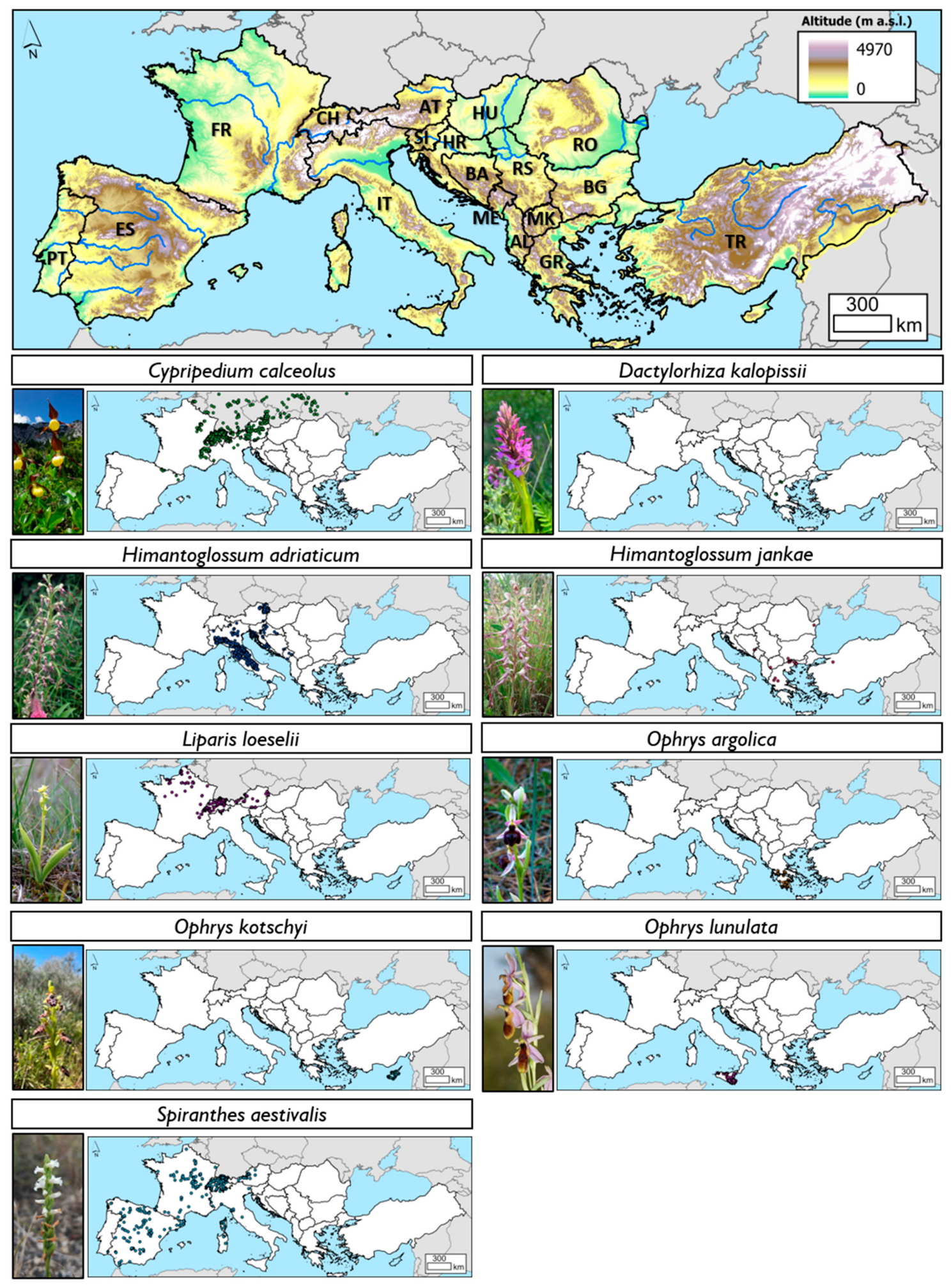
A standardized coordinate-cleaning procedure was subsequently implemented for all species using the R package CoordinateCleaner (v. 3.0.1) [59], which enabled the removal of duplicate records and those flagged as potentially erroneous, including points falling on centroids of administrative units, herbaria, or urban areas. The remaining coordinates were then subjected to a manual point-by-point verification using a Geographic Information System: ArcGIS Pro v. 3.2 [60]. The final dataset with the filtered presences (GBIF occurrence records or points) in the Euro-Mediterranean and surrounding territories is depicted in Figure 1.

Pseudoabsences were generated using the fuzzySim package (v. 4.50) [61], selecting a number ten times greater than the actual presence and ensuring a minimum separation distance of 10 km. Additionally, presence points located within 1 km of another presence were removed in order to reduce spatial autocorrelation.

Figure 1. Study area and filtered presence of the selected orchids. Country codes follow ISO 3166-1 alpha-2 [62]. Orchid’s photographs were obtained from iNaturalist (https://www.inaturalist.org/) under CC-BY licensing.

Figure 1. Study area and filtered presence of the selected orchids. Country codes follow ISO 3166-1 alpha-2 [62]. Orchid’s photographs were obtained from iNaturalist (https://www.inaturalist.org/) under CC-BY licensing.

2.4. Ecological Prediction: Variables

All the variables employed and described below, both “dynamic” and “static”, were projected to a common 1 km² grid under WGS84 (EPSG:4326).

2.4.1. Dynamic Variables

For the purposes of this study, the bioclimatic variables were treated as “dynamic” variables, meaning that their values are expected to shift in the future as a consequence of projected climatic changes under global warming scenarios. In addition to the classical BIO1–BIO19 bioclimatic parameters [63], we included nine bioclimatic indices from the Worldwide Bioclimatic Classification System (WBCS) [64]: continentality index (biorm1 or Ic), compensated thermicity index (biorm2 or Itc), positive temperature (biorm3 or Tp), positive precipitation (biorm4 or Pp), annual ombrothermic index (biorm5 or Io), and summer ombrothermic indices (biorm6, 7, 8, 9 or Ios1, Ios2, Ios3, Ios4, respectively).

For the reference period 1981–2010, monthly mean temperature and monthly total precipitation were obtained from the CHELSA database [65]. The terra R package (v. 1.9-25) [66] was employed to derive the final predictors used in the species distribution modelling.

The climate-change scenarios considered in this study were: SSP2-4.5 2051–2075 (intermediate, mid-term), SSP2-4.5 2076–2100 (intermediate, long-term), SSP5-8.5 2051–2075 (pessimistic, mid-term), and SSP5-8.5 2076–2100 (pessimistic, long-term). Values for all aforementioned variables under these scenarios were obtained from δ-MedBioclim [50]. This database, which applies the delta-change method to ERA5-Land and CHELSA, provides future projections of temperature, precipitation, and bioclimatic variables at the same spatial resolution as their template datasets, for a wide range of CMIP6 General Circulation Models (GCMs).

For the present study, we used an ensemble, based on the CHELSA δ-MedBioclim template, of the best-performing GCMs in the Euro-Mediterranean: GFDL-ESM4, CNRM-CM6-1, CNRM-ESM2-1, IPSL-CM6A-LR, MPI-ESM1-2-HR, and MRI-ESM2-0 for temperature-related variables [34], and CanESM5, CAS-ESM2-0, MPI-ESM1-2-HR, GISS-E2-2-G, HadGEM-GC31-LL, and UKESM1-1-LL for precipitation-related variables [35].

2.4.2. Static Variables

In contrast to the dynamic variables, the modelling of the potential distribution of the selected orchid species also incorporated a set of “static” variables, that is, variables that are not expected to change or, at least, not to a degree that would substantially affect predicted probabilities within the temporal horizons considered.

• Edaphic indicators: Bulk density (BDOD), cation exchange capacity (CEC), volumetric coarse fragments content (CFVO), organic carbon stock (OCS), pH in water (pH) and content of clay (CLC), nitrogen (NC), sand (SAC), silt (SIC), organic carbon (SOC) and volumetric water content (WV0033) values were retrieved from SoilGrids 2.0 [67].
• Topography: Elevation, aspect and slope were derived from the Digital Elevation Model offered by WorldClim [63].
• Solar Radiation: Direct Normal Radiation (DNI), gathered from the Global Solar Atlas 2.0 [68] and the Surface downward solar radiation (RSDS) powered by CHELSA [65], were also incorporated in the distribution modelling.

2.5. Ecological Prediction: Distribution Modelling

The algorithm used to model the potential distribution of the selected orchid species (Table 1) was Bayesian Additive Regression Trees (BARTs) [53]. This machine learning method is implemented in R specifically for Species Distribution Modelling (SDM) through the embarcadero package (v. 1.1) [54]. Its use has increased substantially in recent years, and current evidence suggests that it outperforms deterministic approaches (e.g., GLM, GAM), other ML methods, and even multi-model ensembles [69,70,71,72].

BART was applied at two stages of the modelling workflow. First, it was employed for variable selection through the variable.step() module. This function runs the model i times (where i is the number of predictors) and records the RMSE in each iteration, ultimately selecting the smallest subset of variables that minimizes prediction error. This procedure prevents issues associated with multicollinearity and provides an objective, data-driven framework for predictor selection. The varimp() function complements this process by quantifying the relative importance of each predictor.

Default parameters were used: 200 trees, 1000 posterior draws, and 100 Markov Chain Monte Carlo interactions. However, the retune() function was implemented to evaluate potential improvements under alternative parameterizations.

Finally, for the generation of binary suitability—as non-suitability maps were required for the vulnerability analysis—we applied the threshold maximizing the True Skill Statistic (TSS). Changes in potential area were assessed by comparing present conditions (reference period 1981–2010) with future projections (for each of the scenarios considered). The area maintained in the future (M) is defined, for the purposes of this study, as the proportion of currently suitable area that remains suitable under future conditions (FPA∩CPA)/CPA. The area lost (L) is defined as 100−M. Finally, the area gained corresponds to areas that are suitable in the future but not under present conditions, expressed as (FPA∪CPA)/CPA. These results are presented as maps produced using the ETRS89 LAEA projection (EPSG:3035) using ArcGIS Pro v3.2 [60].

2.6. Vulnerability Assessment

To assess the vulnerability of each orchid species under the different scenarios analyzed, we applied a vulnerability analysis using the vulnerability index (VI) proposed by Felicísimo et al. (2012) [73] and subsequently modified by del Río et al. (2021) [51] (Equation (1)). This index compares the future potential area (FPA) with the current occupied area (COA) and with the current potential area (CPA) to evaluate how intense the potential retraction (or extension) of suitable habitat could be.

$$VI=1-(FPA\cap COA)\times (FPA\cap CPA)$$

(1)

However, with the aim of ensuring that the results of the present study can serve as a complementary criterion for the future assignment of threat categories to the species analyzed, we adapted the categories proposed by the aforementioned authors to align with the terminology employed by the IUCN, as follows:

• VI < 0.00: Not at risk (“climate change winner”).
• 0.00 < VI < 0.40: Least Concern (LC).
• 0.40 < VI < 0.70: Near Threatened (NT).
• 0.70 < VI < 0.85: Vulnerable (VU).
• 0.85 < VI < 0.95: Endangered (EN).
• VI > 0.95: Critically endangered (CR).

Nevertheless, it should be noted that this vulnerability index considers only the intersection between the future potential area, the area currently occupied by the species, and the area it could potentially occupy, without accounting for newly gained suitable areas. As a result, it may lead to an overestimation of vulnerability, which should be taken into consideration when interpreting the results.

3. Results

3.1. BART Model Assessment

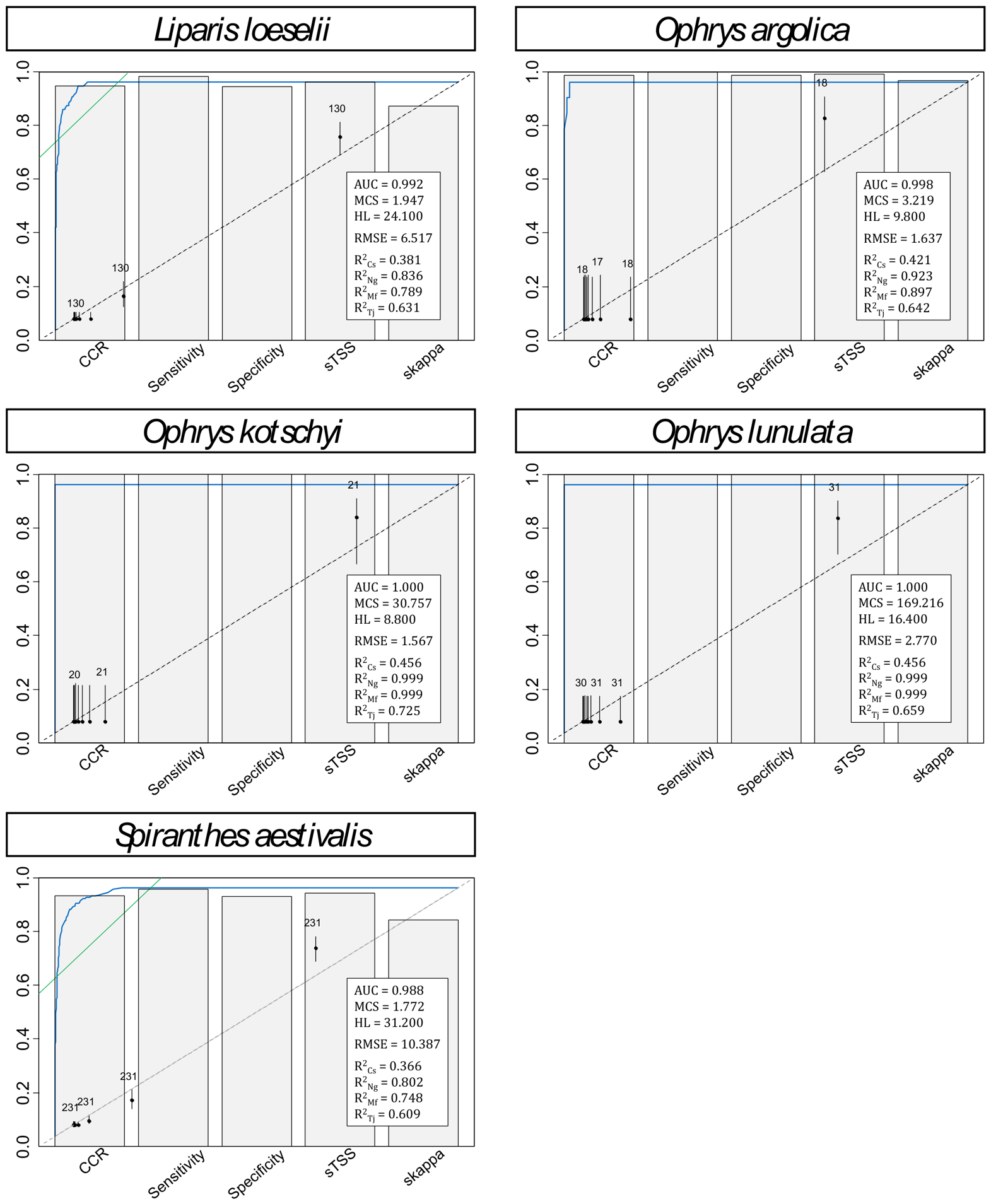
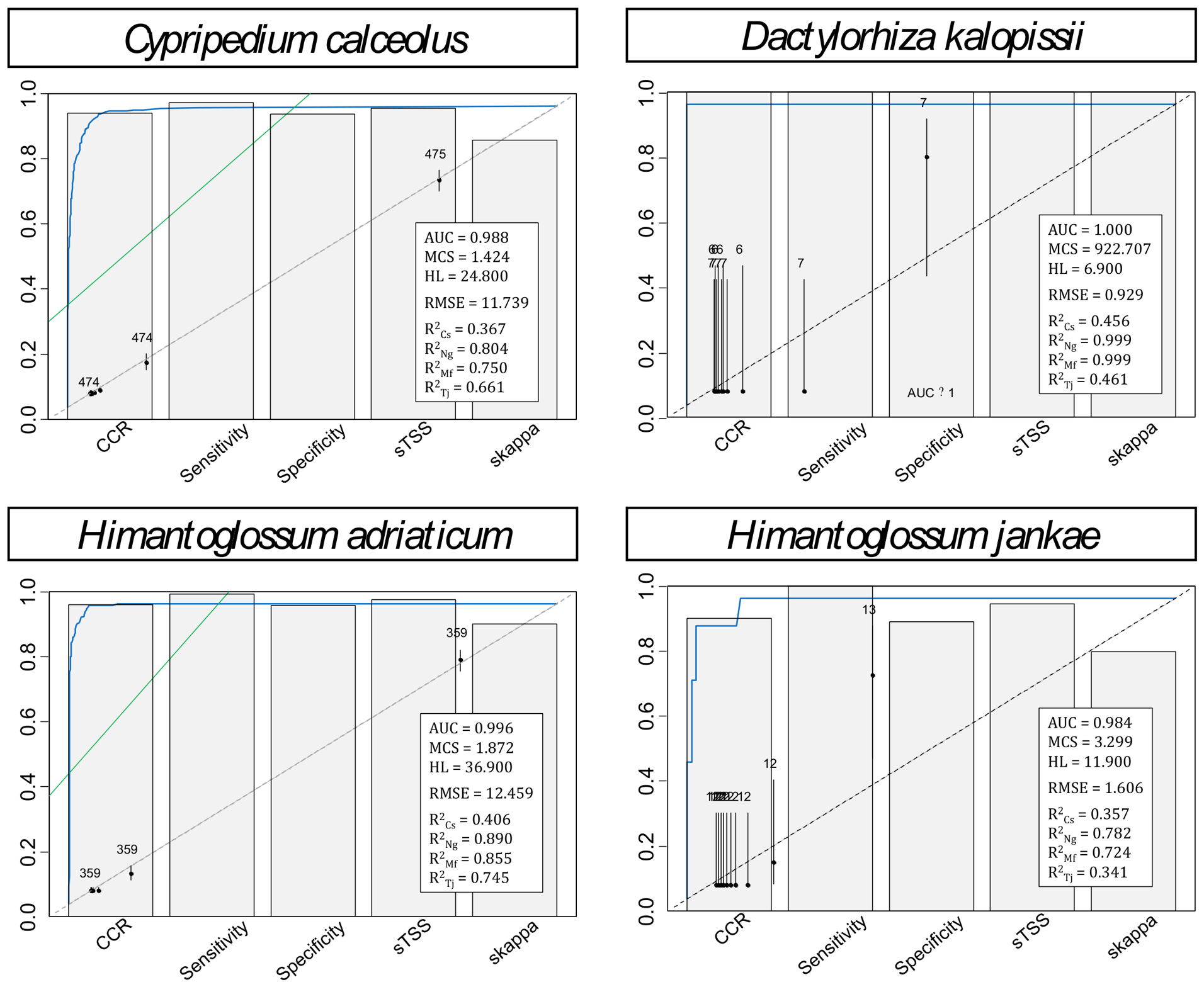
In Figure A1 (Appendix A), the principal discrimination, classification, calibration, and correlation metrics are presented for the models generated using the BART algorithm for each of the species under study. All models exhibit a pattern where discrimination (AUC > 0.98) and classification (TSS > 0.8) performance can be interpreted as satisfactory. However, except for C. calceolus (MCS = 1.42), H. adriaticum (MCS = 1.87), and S. aestivalis (MCS = 1.77), calibration is generally poor, and even for these species, a slight overestimation is detectable. These three species correspond to those with a relatively high number of presences within the study area (n > 200).

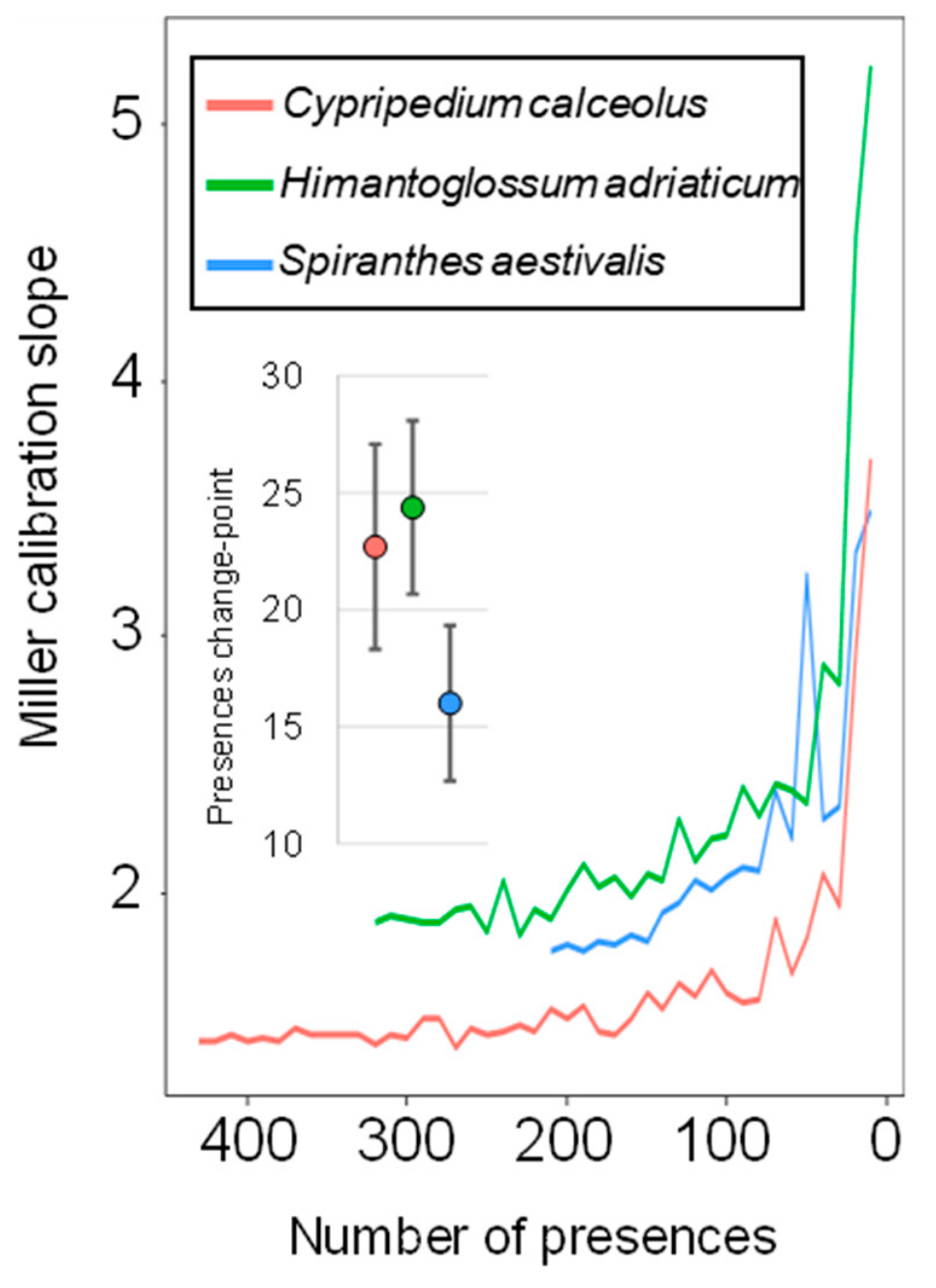
Figure 2 illustrates this issue: several BART models were sequentially fitted after a controlled removal of presences (and consequently of pseudo-absences) for our three orchids with n > 200. The results show that although calibration, measured using the Miller calibration slope (MCS), is acceptable (MCS < 2) at the full sample size, it increases markedly as presences are removed. The detected number of presences change-point beyond which MCS values escalate varies slightly among species: C. calceolus (22.69 [18.31–27.07]) and H. adriaticum (24.37 [20.66–28.08]) would require a larger sample size to maintain adequate calibration, whereas S. aestivalis (16.00 [12.68–19.32]) appears to require fewer presences.

Having detected this lack of calibration, future projections will only be established for C. calceolus, H. adriaticum, L. loeselii and S. aestivalis (MCS < 2.0), with particular caution for these latter two (1.7 < MCS < 2.0).

3.2. Environmental Predictors of Distribution

Table 2. Variable importance (%) for each analyzed species. The number in brackets indicates the rank (from 1st to 5th) occupied by each variable. Spatial dependence plots of the five most important predictors are depicted in Figure A2 (Appendix A). See Section 2.4 for predictor abbreviations. Cy.ca.: Cypripedium calceolus; Da.ka: Dactylorhiza kalopissii; Hi.ad: Himantoglossum adriacticum; Hi.ja: Himantoglossum jankae; Li.lo: Liparis loeselii; Op.ar.: Ophrys argolica; Op.ko.: Ophrys kotschyi; Op.lu.: Ophrys lunulata; Sp.ae.: Spiranthes aestivalis.

	Cy.ca.	Da.ka.	Hi.ad.	Hi.ja.	Li.lo.	Op.ar.	Op.ko.	Op.lu.	Sp.ae.
BIO1	-	-	-	-	9.53	-	-	-	-
BIO4	8.36	-	9.18 (3)	-	9.84 (4)	-	-	-	10.52 (2)
BIO8	-	-	-	-	-	-	-	20.29 (3)	-
BIO9	9.14 (2)	-	8.45 (5)	-	9.73	-	-	-	-
BIO11	-	-	8.38	-	-	-	17.46 (1)	-	9.08
BIO13	8.20	-	-	-	-	11.97	16.43 (5)	-	-
BIO15	-	-	8.82 (4)	-	-	-	14.88	-	-
BIO16	7.90	-	-	-	-	12.64 (3)	16.72 (4)	-	-
BIORM1	7.60	34.28 (1)	7.96	-	10.16 (3)	-	-	20.45 (2)	-
BIORM3	-	-	-	-	9.65	-	-	-	-
BIORM4	-	-	-	-	-	12.88 (1)	-	-	-
BIORM6	-	-	-	-	9.61	-	-	-	10.15 (4)
BIORM7	7.92	-	-	-	-	-	-	18.53 (5)	-
BDOD	-	-	8.17	-	-	-	-	-	-
CEC	-		-	-	-	12.34	-	-	-
CFVO	8.38 (5)	-	-	-	10.69 (2)	-	17.32 (2)	-	10.30 (3)
CLC	8.40 (4)	-	-	-	-	-	-	-	10.06 (5)
OCD	7.96	-	7.58	-	9.78 (5)	-	-	-	9.38
NC	-	-	-	26.17 (1)	-	-	-	-	-
pH	-	-	7.32	-	-	-	-	-	9.46
SAC	-	-	7.94	25.76 (2)	-	-	-	-	-
SIC	7.74	-	-	-	-	-	-	-	-
WV	-	-	-	-	-	12.39 (5)	-	-	-
DNI	-	-	9.32 (1)	24.70 (3)	-	12.59 (4)	-	19.19 (4)	9.93
RSDS	9.86 (1)	33.31 (2)	9.26 (2)	-	10.99 (1)	12.84 (2)	17.19 (3)	21.54 (1)	11.42 (1)
Altitude	8.56 (3)	32.42 (3)	-	-	-	-	-	-	9.71
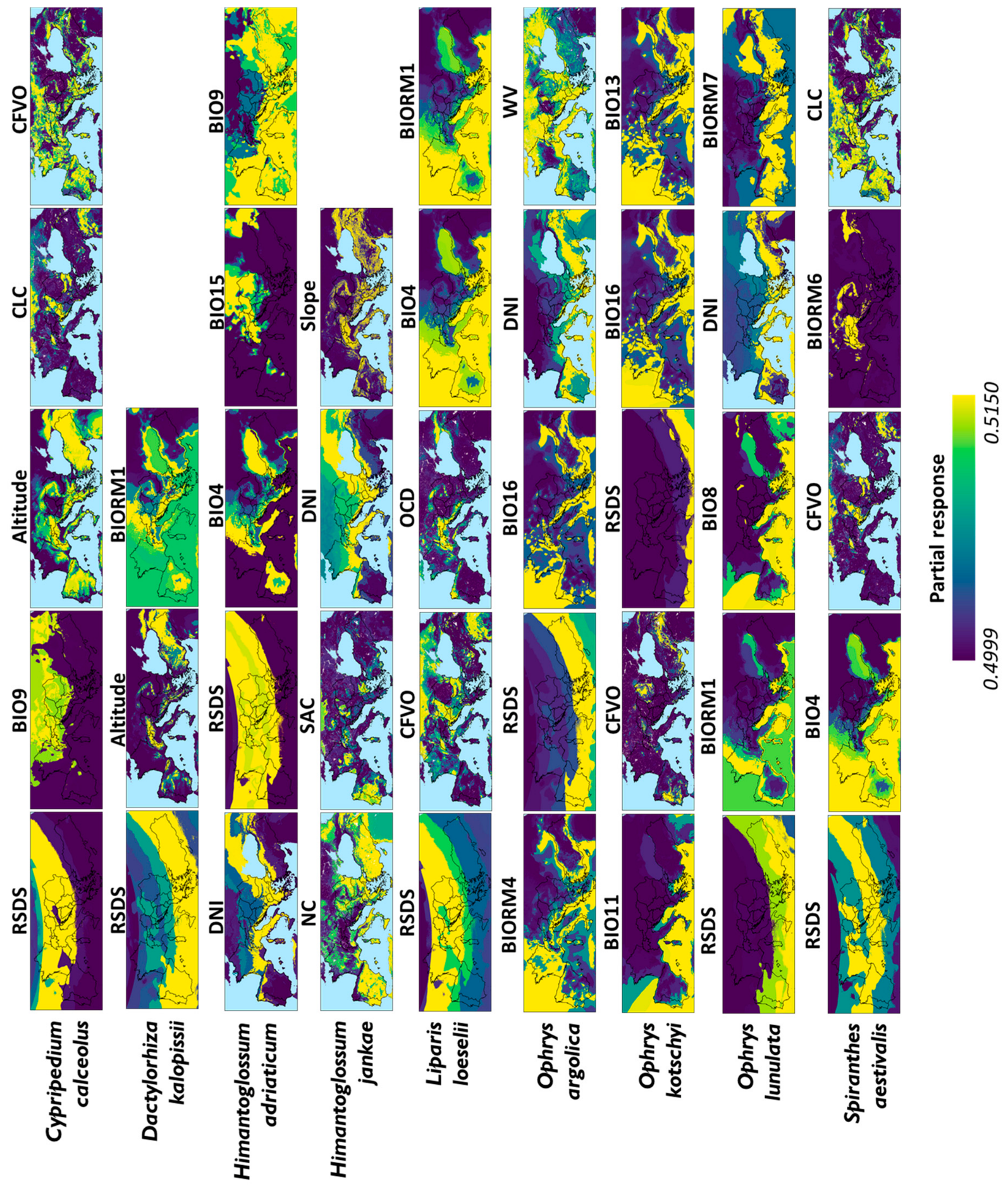
Slope	-	-	7.63	24.38 (4)	-	12.34	-	-	-

summarizes the variables identified by BART as relevant for each of the analyzed species, revealing both shared patterns and marked interspecific differences in the drivers of potential distribution. Their relative importance, quantified as the number of times each variable was used to split a tree branch and subsequently standardized as a percentage, is also disclosed.

Climatic variables, particularly those related to temperature and precipitation, show varying importance depending on the species. Among temperature-related predictors, BIO4 (temperature seasonality) emerges as a relevant factor for several taxa, including C. calceolus, H. adriaticum, L. loeselii, and S. aestivalis. Similarly, BIO9 (mean temperature of driest quarter) and BIO11 (mean temperature of coldest quarter) also contribute to explaining species distributions, although in a more species-specific manner (e.g., H. adriaticum). In contrast, BIO1 (annual mean temperature) shows limited importance, being relevant only for L. loeselii, which may reflect the greater influence of seasonal extremes rather than mean conditions.

Precipitation-related variables display a similarly uneven pattern. BIO13 (precipitation during the wettest month) and BIO16 (precipitation during the wettest quarter) are particularly important for O. argolica and O. kotschyi, as well as for C. calceolus, indicating the relevance of water availability during critical periods. Additionally, BIO15 (precipitation seasonality) contributes to explaining the distribution of H. adriaticum and O. kotschyi, reinforcing the role of intra-annual variability in precipitation regimes.

Finally, bioclimatic indices (BIORM variables) further refine this picture, with BIORM1 (continentality index) standing out as a dominant predictor for D. kalopissii and O. lunulata, as well as a selected variable for C. calceolus, H. adriaticum or L. loeselii. Furthermore, “mixed” bioclimatic indices (i.e., those integrating both temperature and precipitation components) such as BIORM6 (ombrothermic index of the warmest summer month) and BIORM7 (ombrothermic index of the warmest summer bimester), emerge as relevant predictors for several species. Specifically, BIORM6 is influential for L. loeselii and S. aestivalis, whereas BIORM7 plays a significant role in explaining the distributions of C. calceolus and O. lunulata.

Edaphic variables show a strong influence on specific species, underlining the importance of soil properties in orchid ecology. Organic carbon (OCD) and coarse fragments (CFVO) are relevant for several taxa, including C. calceolus, L. loeselii, and S. aestivalis, while pH and bulk density (BDOD) contribute to explaining the distribution of H. adriaticum and S. aestivalis. Notably, nitrogen content (NC) and sand content (SAC) emerge as the dominant predictors for H. jankae, clearly distinguishing it from the rest of the species and suggesting a strong dependence on specific soil nutrient conditions. Clay content (CLC) and other environmental descriptors such as volumetric water content (WV) and cation exchange capacity (CEC) show moderate importance in a limited number of species, particularly C. calceolus, O. argolica, and S. aestivalis.

The most influential predictors are those related to solar radiation. In particular, surface downwelling shortwave radiation (RSDS) is the top-ranked predictor for multiple taxa, including C. calceolus, L. loeselii, O. lunulata, and S. aestivalis, and remains among the most influential variables in nearly all cases (except for H. jankae). Direct normal irradiance (DNI) was retained for five taxa and emerged as the strongest predictor for H. adriaticum.

Finally, topographic variables do not seem to play a crucial role in the distribution of selected orchids. However, altitude contributes notably to the distribution of C. calceolus, D. kalopissii, and S. aestivalis, while slope, although less consistently important, plays a role in H. adriaticum and H. jankae.

3.3. Forecasting Habitat Potential Shifts

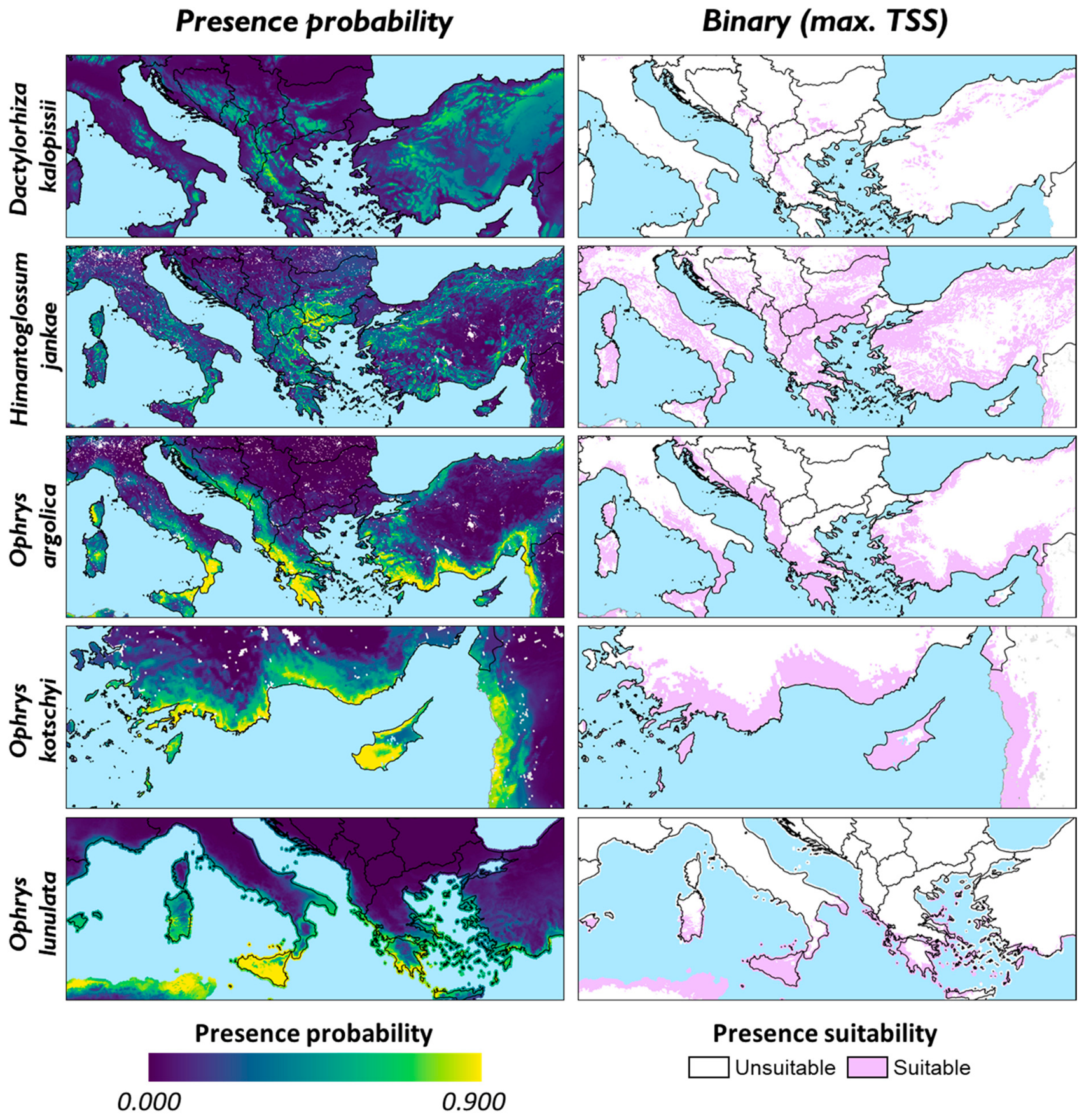
Due to the impossibility of obtaining adequately calibrated models for D. kalopissii, O. kotschyi, O. argolica, and O. lunulata, the uncertainty associated with future predictive models was considered excessively high, thereby substantially limiting their usefulness. For completeness, their current potential distribution is shown in Figure A3 (Appendix A). Similarly, no dynamic variable proved informative for predicting the distribution of H. jankae; consequently, its projected distribution models would be identical to those of the present period (Figure A3; Appendix A).

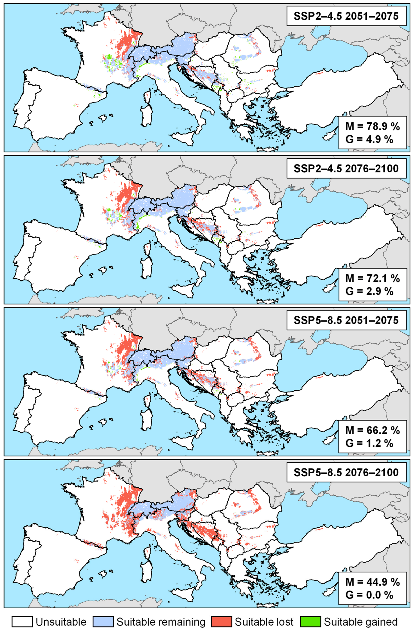
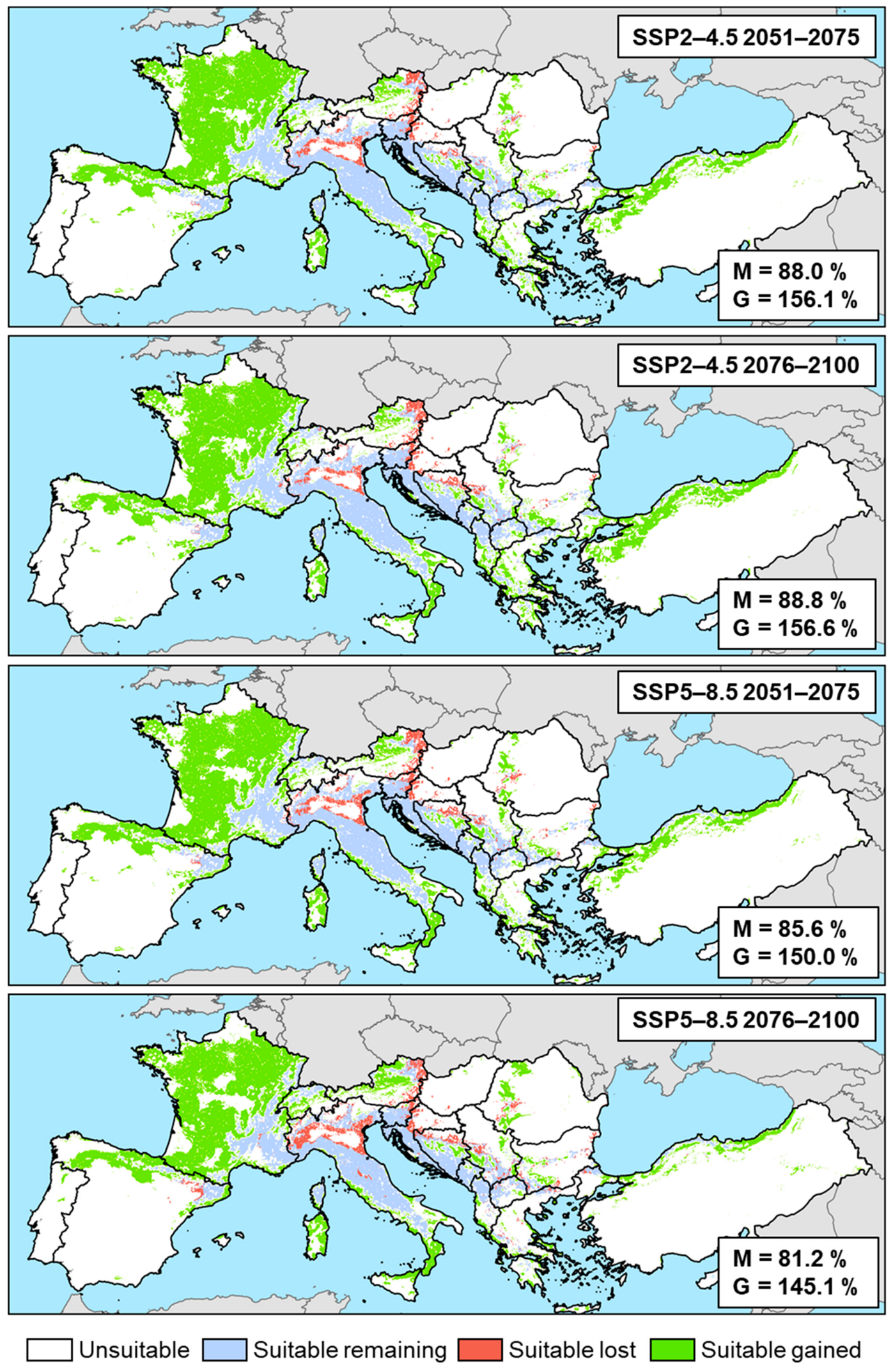
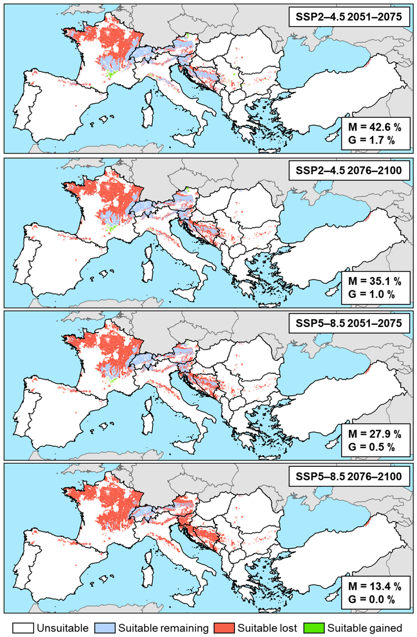
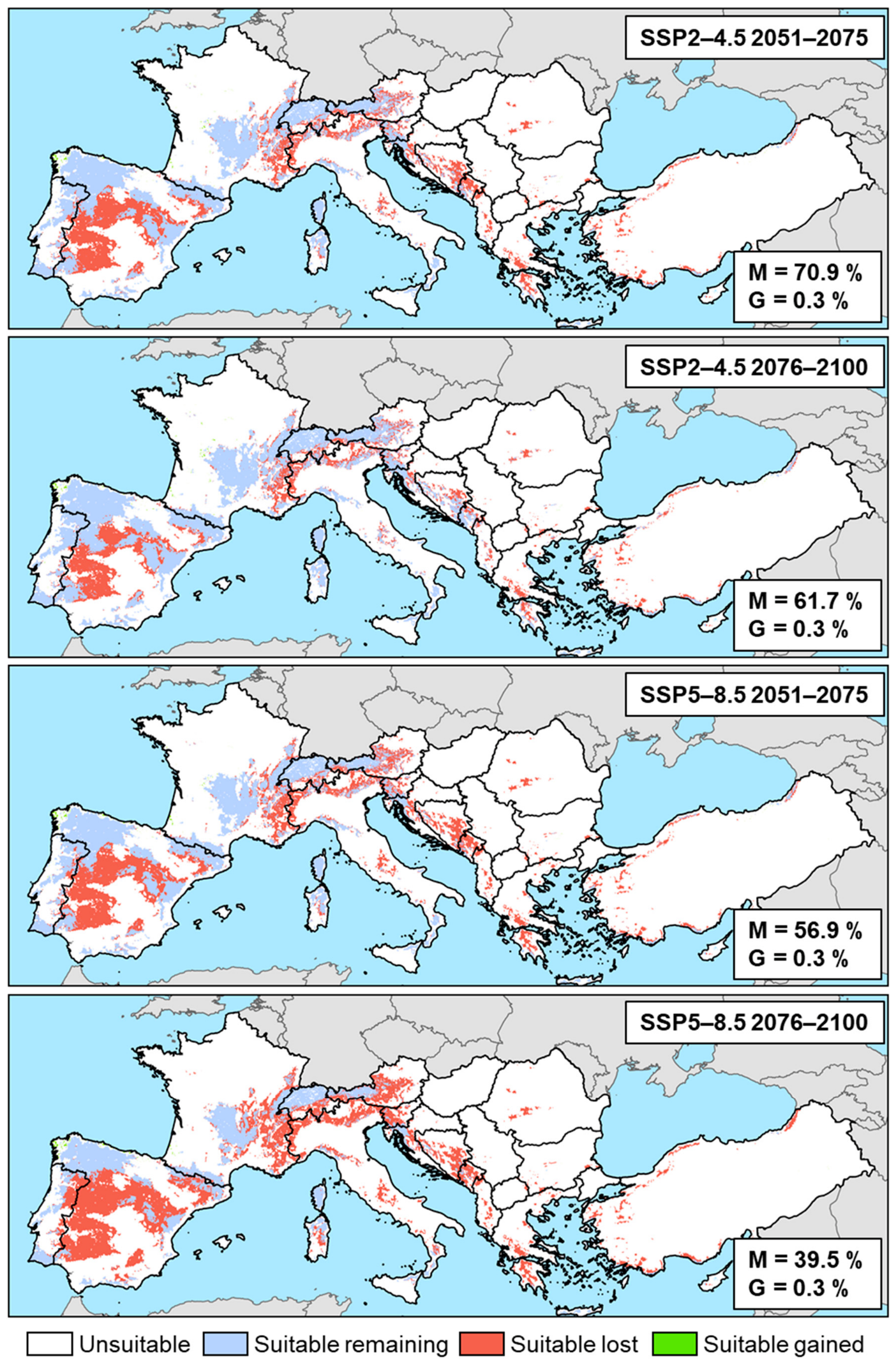
Accordingly, Figure 3, Figure 4, Figure 5 and Figure 6 present the projected potential distribution under the selected scenarios (SSP2-4.5 2051–2075, SSP2-4.5 2076–2100, SSP5-8.5 2051–2075, SSP5-8.5 2076–2100) for C. calceolus, H. adriaticum, L. loeselii, and S. aestivalis. The color code used in these figures indicates: in blue, areas currently suitable that remain suitable in the future (M = 1–1); in red, areas currently suitable that are projected to be lost (L = 1–0); and in green, areas that are not currently suitable but are projected to become suitable in the future (G = 0–1). The reader should note that the sum of blue and red areas corresponds to the suitable area during the reference period (1981–2010).

Cypripedium calceolus is projected to experience a marked potential contraction of its current distribution, ranging from approximately 21% under the most optimistic scenario to up to 55% under the most pessimistic one (Figure 3). The Alpine range appears to be the most resilient area, particularly in the central–eastern Swiss–Austrian sector. The most pronounced losses are expected in northeastern France (Jura and Vosges). In the Pyrenean range, which hosts the southernmost relict populations, losses could be of particular concern, especially under the SSP5-8.5 scenario. Under this scenario, substantial declines are also projected in the Dinarides and the Carpathians; these regions could potentially host populations of the species where, based on the presence data used (Figure 1), the species is currently absent.

The case of H. adriaticum is markedly different (Figure 4). This species is projected to retain more than 80% of its current potential distribution under all scenarios, while also exhibiting a potential gain exceeding 50%. Losses are expected to be concentrated primarily in the Po Valley, while gains are projected in France and in northern Spain and Portugal.

Finally, L. loeselii and S. aestivalis fall within the group of species that could be negatively affected by climate change. For L. loeselii (Figure 5), although potential habitat appears to persist within the Alpine range, it is projected to disappear from northern France under all scenarios. Estimated losses range from approximately 60% (SSP2-4.5, mid-term) to more than 85% (SSP5-8.5, long-term), with the loss of potentially suitable areas in the Dinarides and the Apennines as well. For S. aestivalis (Figure 6), although the projected loss of potential habitat is comparatively lower (between 30% and 60%), potential gains are equally negligible (approximately 0.3% under all scenarios). The central–southern Iberian Peninsula and subalpine regions appear to be particularly affected.

3.4. Climate Change Vulnerability

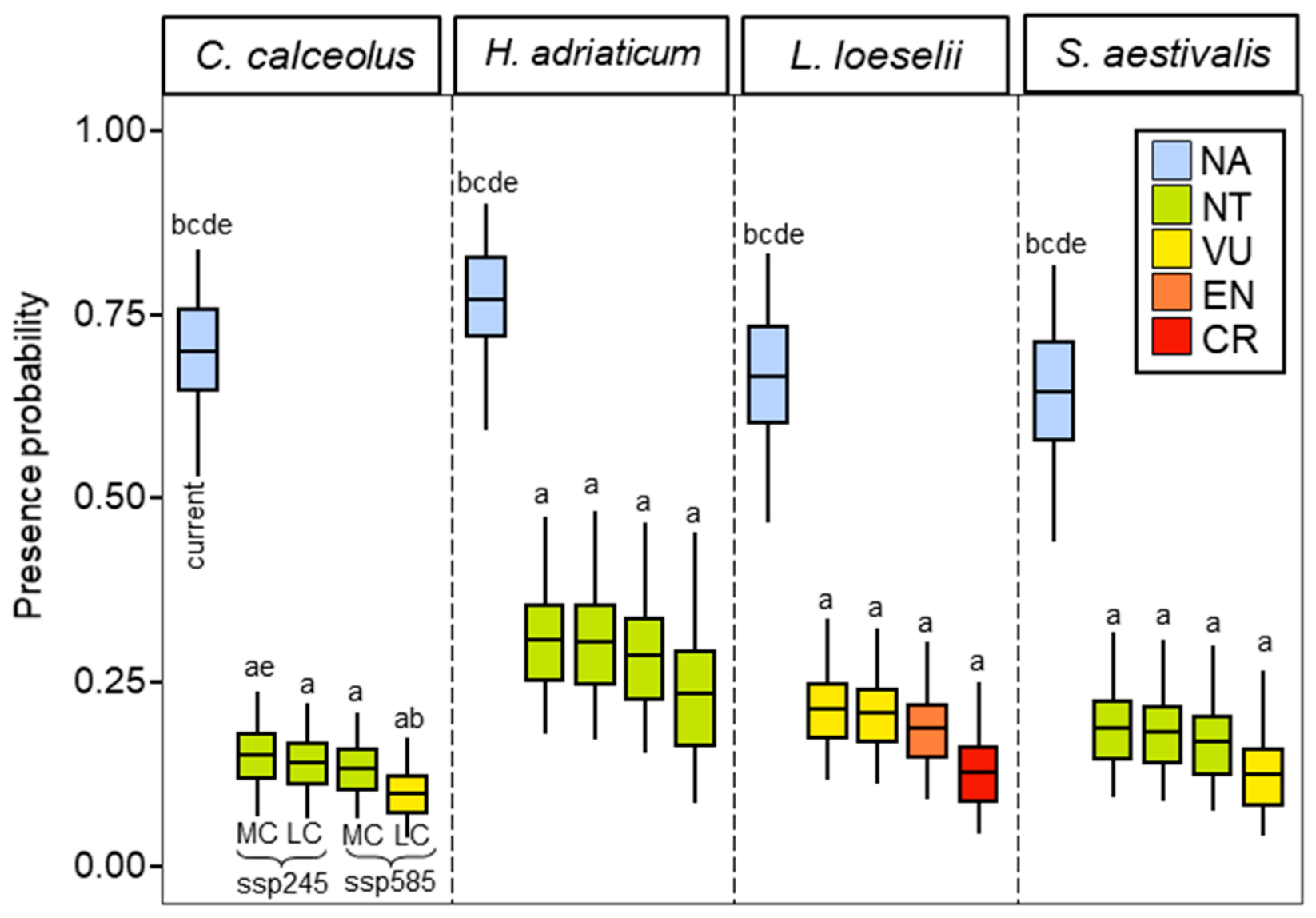
The vulnerability analysis for the four modeled species is presented in Figure 7. Under all scenarios considered, all species are projected to experience not only a spatial contraction (Figure 3, Figure 4, Figure 5 and Figure 6) but also a statistically significant decrease in predicted probability of presence.

In the case of H. adriaticum, an expansion of suitable areas is projected under future scenarios (Figure 4). However, this is coupled with a marked decline in habitat suitability, as reflected by a reduction in the median predicted probability of presence from approximately 75% under current conditions to between 25% and 40% in all future scenarios. Nevertheless, its threat status does not worsen beyond Near Threatened.

In contrast, C. calceolus is the only species for which statistically significant differences among scenarios are detected. Under the long-term pessimistic scenario (SSP5-8.5, 2076–2100), the species exhibits a significantly greater decline in predicted probability of presence compared to the intermediate mid-term scenario (SSP2-4.5, 2051–2075). This reduction is sufficient to shift its threat category from Near Threatened to Vulnerable. A similar tendency is observed for S. aestivalis, although differences among scenarios are not statistically significant; notably, the species is classified as Vulnerable only under the long-term pessimistic scenario.

Finally, among the analysed species, L. loeselii emerges as the most climatically vulnerable. It is classified as Vulnerable under all SSP2 scenarios, while under SSP5 scenarios, its status worsens to Endangered in the medium term and Critically Endangered in the long term.

4. Discussion

4.1. Sample Size and Other Limitations on Model Performance

In this specific case study, the assessment of the BART models suggests a clear loss of calibration capacity when the number of presences is low. This finding is consistent with earlier studies that reported a decline in model performance with decreasing sample size, concluding that no modeling approach exhibits consistent performance for n < 30 [74]. More recent research has further emphasized that the minimum required sample size is strongly dependent on species prevalence [75], while the most recent review indicates that only a minority of studies recommend working with n < 50 [76]. That same review highlights predictor selection and model complexity as critical factors, particularly due to their potential to induce over- or underestimation. In the present study, however, both aspects were considered adequately addressed within the applied BART framework.

Therefore, the differences in model performance among the study species may also be attributable to their ecological characteristics. Specifically, species with a more generalist ecology and broader environmental niche may be less prone to calibration issues such as spatial autocorrelation. Indeed, previous hypotheses suggest that minimum sample size requirements are not fixed but instead depend on species’ ecological traits as well as stochastic factors such as prevalence [75,76]. In conclusion, we concur with the view that species distribution models (SDMs) for species with very low prevalence are of limited utility and, specifically, we cannot recommend, in light of our results, generating models with n ≤ 20.

Moreover, the implemented dataset could also render non-negligible uncertainties. Indeed, over the past decades, GBIF has become the most widely used biodiversity database worldwide [77]. However, these strengths are not without limitations: sampling bias, erroneous human observations or misidentifications, dataset/metadata incompleteness, and limited spatial or temporal accuracy in certain regions are among the most frequently cited issues and should be carefully considered when interpreting the results obtained [78,79]. In this regard, model outputs should be interpreted as approximations of environmentally suitable conditions rather than exhaustive representations of species distributions, particularly in under-sampled areas. Nevertheless, the use of herbarium-based records [79], combined with manual verification procedures and the flexibility of the species distribution modelling approach applied here, may provide sufficiently robust safeguards to mitigate potential biases present in the initial dataset.

4.2. Environmental Drivers of Euro-Mediterranean Orchid Distribution

Our study reveals notable differences in the variables that appear to affect the studied orchid species to a greater or lesser extent, suggesting potential variation in the ecological niches occupied by each of them. This is consistent with the wide diversity of niches present in a biogeographically complex region such as the Euro-Mediterranean. Nevertheless, certain patterns, such as the importance of solar radiation and continentality, appear to be consistent across the vast majority of the cases analyzed.

Firstly, the ecological association of the studied species with heliophilous grassland and shrubland communities provides a clear explanation for the prominence of radiation-related variables [42,80]. In addition, both RSDS and DNI are strongly correlated with latitude, which has been identified as a key factor explaining orchid diversity patterns [39].

Temperature-related variables, like the continentality index, also play an important role, as they reflect climatic harshness and the magnitude of thermal contrasts between maximum and minimum temperatures: factors previously reported as relevant for orchid distribution [42,43,46]. For example, mean thermal amplitudes of approximately 5 °C have been described as characteristic of Australian orchid habitats [43]. On the other hand, precipitation variables also emerge as relevant predictors in several cases. In a modeling study of three Italian orchid species, BIO4 (temperature seasonality) was influential only for Limodorum abortivum (L.) Sw., whereas the remaining species were primarily driven by precipitation-related or edaphic variables [46]. Similarly, the Greek endemic Ophrys helenae Renz has been shown to be strongly associated with precipitation during the wettest quarter (BIO16) [38]. In the present study, BIO16 was also identified as relevant for C. calceolus, a temperate obligate species with a preference for higher elevations, as well as for O. argolica and O. kotschyi, which are Greek and Cypriot endemics, typically occurring under much drier climatic conditions.

In terms of edaphic variables, they have also been highlighted as key determinants of orchid distribution. A case study on Cypripedium species in North America identified soil taxonomy as the strongest predictor of habitat suitability [44], while the aforementioned study on Ophrys helenae emphasized soil carbon content as a key factor [38]. A plausible explanation lies in the relationship between soil texture, organic matter content, and the richness and composition of mycorrhizal communities [16,17,81]. These endosymbiotic associations are essential for the survival of terrestrial orchids and constitute one of the primary limiting factors for their distribution [45]. Accordingly, organic soil carbon has already been identified as an important predictor of orchid germination and distribution [82].

Particularly noteworthy is the case of H. jankae, the only species in this study for which soil nitrogen (NC) emerged as a key determinant. This finding is consistent with experimental evidence indicating that its germination is amino acid-dependent [83]. The direct relationship between SDMs and germination experiments has also been previously explored in orchids [82], further supporting the ecological relevance of this result.

However, the potential taxonomic uncertainty between Himantoglossum jankae and Himantoglossum caprinum (M. Bieb.) Spreng. warrants careful consideration when interpreting the results obtained for H. jankae. Misidentifications between both taxa have been suggested to be common, even more so before the description of H. jankae [84]. Therefore, some occurrences recorded in GBIF under H. caprinum may in fact correspond to H. jankae, contributing to an underestimation of the true number of presences for H. jankae, and thereby affecting model performance. Consequently, these results should be interpreted with caution, and future studies incorporating taxonomically validated occurrence data would be necessary to improve model reliability in this regard.

In contrast, a recent large-scale study modeling 107 European orchid species using MaxEnt reported that soil- and precipitation-related variables were of comparatively lower importance, classifying orchids into two main groups: temperature-dependent and land-cover-dependent species [85]. Of the nine species analyzed here, six were also included in that study. Specifically, D. kalopissii and O. lunulata were classified as temperature-dependent, in agreement with our results identifying the continentality index as their strongest predictor, with BIO8 (mean temperature of wettest quarter) also relevant for O. lunulata. C. calceolus, L. loeselii, and S. aestivalis were classified as land-cover-dependent, whereas O. argolica, identified in our models as primarily driven by biorm4 (positive precipitation), along with BIO13 (precipitation of wettest month) and BIO16 (precipitation of wettest quarter), was also categorized as land-cover-dependent but within a precipitation-driven subcluster.

Finally, the relatively coarse resolution of topographical variables (1 km) could obscure the influence of variables such as slope or aspect that are relevant to orchid settlement, but only at microhabitat scales [82]. This suggests, therefore, that an information loss process may occur as a consequence of spatial aggregation [86,87,88].

4.3. Projected Distribution Shifts and Conservation Implications

The predictive models generated in this work are far from perfect. Assumptions inherent to Species Distribution Modeling protocols (e.g., noise assumptions) or the potential emergence of future non-analog conditions (combinations of variables producing environments fundamentally different from those used to train the models) inevitably affect the results and their interpretation [89]. Nevertheless, their usefulness in biodiversity management and land-use planning is well established [90,91], including in the specific case of orchids [46,92].

Regarding future projections, the estimates for C. calceolus are consistent, although more conservative, than those reported in previous modeling studies [93], as well as the declines predicted for other species of the genus in North America [44].

In the case of H. adriaticum, projected losses are expected to be concentrated primarily in the Po Valley, where an increase in xeric temperate bioclimates is anticipated [94]. This increase in continentality is likely to be detrimental to a species tending toward oceanicity [95]. Additionally, the reduction in frost days associated with increasing temperatures, identified as the most strongly correlated variable with reproductive success [96], provides a plausible explanatory mechanism. At the same time, its heat requirements are aligned with Mediterranean conditions, as the species inhabits dry grasslands of the Festuco-Brometea class. Therefore, the expansion of sub-Mediterranean conditions into currently temperate regions may partially favor its distribution [95].

Nevertheless, when referring to the expansion of potential distribution areas in species that are highly dependent on interspecific interactions to complete their life cycle, the potential viability of their dispersal or pollination agents should also be considered. In other words, in the case of H. adriaticum, it is possible that areas identified as suitable for future expansion may not be accessible to its pollinators, thereby severely limiting its actual viability. This represents an important limitation that is not addressed in our study. For instance, in the mycoheterotrophic orchid Limodorum abortivum, it has been shown that although its potential habitat may expand under future conditions, fewer than half of its populations (20% under pessimistic scenarios) would overlap with the potential distribution of its main pollinator, preventing successful establishment [19]. A similar pattern was reported by Tsiftsis and Djordjevic [97], who even predict the extinction of Ophrys delphinensis O. Danesch & E. Danesch due to the absence of overlap with its sole pollinator, Anthophora plagiata (Illiger, 1806). Even in species with a relatively broad range of pollinators, such as H. adriaticum [96], the extent of suitable areas could be substantially reduced by the concerning decline in pollinator availability discussed in previous sections [20,21,22].

Regarding S. aestivalis, conservation assessments in Spain describe it as a supra-orotemperate species with high water requirements [98]. The projected expansion of Mediterranean and submediterranean conditions [94], together with reduced water availability [99], offers a plausible explanation for the predicted distributional changes. Moreover, the ombrothermic index of the warmest month (Ios1 or biorm5) was identified as a key variable influencing its distribution. Nevertheless, further research on its habitat requirements is needed, as the species is not only climatically vulnerable but also affected by additional pressures such as grazing and water pollution [98].

Finally, for L. loeselii, previous studies have identified soil eutrophication and drainage as the main drivers of its decline [100,101]. The present results suggest a compounded risk scenario, in which significant climatic vulnerability is added to these existing threats. Moreover, its limited capacity to colonize new environments, as reported in earlier studies [101], is consistent with the marginal gains observed in our projections, which remain below 1.5% and are null under the most pessimistic scenario.

For more than a decade, the literature has converged on the need for integrated management approaches to conserve such a diverse and threatened group [102]. More interventionist measures should be combined with strengthened legal protection and habitat-level actions aimed at enhancing the presence of species-specific pollinators [47]. Proper maintenance of ex situ collections, with genetic variability representative of natural populations, in botanical gardens and germplasm banks is also essential [47,103,104]. This ensures that "extinction in the wild does not equate to global extinction". Recent studies identifying 278 priority orchid species report that only approximately 25% are currently represented in botanical gardens [103].

Furthermore, the limited dispersal capacity of many orchid species necessitates artificial assistance to overcome ecological barriers [102]. Such translocations or assisted migrations, informed by SDM outputs, can be directed toward areas where environmental favorability is known to be high [92]. Increased monitoring and environmental education efforts are likewise essential, particularly for species occurring in highly human-disturbed ecosystems [104]. These areas require enhanced protection and controlled disturbance regimes, especially where future declines or losses of suitability are anticipated. Finally, ensuring strict compliance with the CITES agreement in the commercial trade of orchids, particularly those that are most vulnerable or exposed to multiple threat factors, is critical to safeguarding this exceptionally valuable component of our natural heritage for future generations [104].

5. Conclusions

This study provides a Bayesian Additive Regression Trees (BARTs) modeling-based assessment of the potential impacts of climate change (under medium- and long-term intermediate and pessimistic scenarios) on orchid species listed under Directive 92/43/EEC.

The results indicate that model performance is strongly constrained by sample size, with calibration becoming unreliable below approximately 16–25 presence records, a threshold that appears to depend on the ecological tolerance of species. Among the environmental drivers considered, solar radiation emerged as the most influential variable shaping orchid distributions, while continentality and key edaphic (particularly CFVO and OCD) properties also played a significant role. It underscores the importance of integrating both climatic/bioclimatic and soil-related factors.

Projections under future climate scenarios reveal a potential generalized contraction of suitable habitats for several species, particularly Liparis loeselii (57–87%), Cypripedium calceolus (20–55%), and Spiranthes aestivalis (29–60%), with more pronounced losses under long-term and high-emission scenarios. Under these hypotheses, Liparis loeselii could reach a Critically Endangered status. In contrast, Himantoglossum adriaticum may exhibit relative stability or even potential expansion. These contrasting responses suggest that climate change will not affect orchid species uniformly, but will instead amplify differences in vulnerability among taxa.

Overall, these findings highlight the value of bioclimatic modeling as a tool to anticipate species-specific responses to climate change and support forward-looking conservation strategies. In particular, the identification of areas of future climatic suitability may contribute to more effective conservation planning, including the prioritization of protection measures and the potential implementation of assisted migration where appropriate.

References

1. Christenhusz, M.; Byng, J.W. The Number of Known Plant Species in the World and Its Annual Increase. Phytotaxa 2016, 261, 201–217. [Google Scholar] [CrossRef]
2. Givnish, T.J.; Spalink, D.; Ames, M.; Lyon, S.P.; Hunter, S.J.; Zuluaga, A.; Doucette, A.; Caro, G.G.; McDaniel, J.; Clements, M.A.; et al. Orchid Historical Biogeography, Diversification, Antarctica and the Paradox of Orchid Dispersal. J. Biogeogr. 2016, 43, 1905–1916. [Google Scholar] [CrossRef]
3. Pérez-Escobar, O.A.; Bogarín, D.; Przelomska, N.A.S.; Ackerman, J.D.; Balbuena, J.A.; Bellot, S.; Bühlmann, R.P.; Cabrera, B.; Cano, J.A.; Charitonidou, M.; et al. The Origin and Speciation of Orchids. New Phytol. 2024, 242, 700–716. [Google Scholar] [CrossRef]
4. Euro+Med. Euro+Med PlantBase—The Information Resource for Euro-Mediterranean Plant Diversity. Available online: https://europlusmed.org/ (accessed on 21 November 2025).
5. Mediterranean Conservation Society Anatolian Orchids Project. Available online: https://akdenizkoruma.org.tr/en/projects/projects/b/anatolian-orchids-project?utm_source=chatgpt.com (accessed on 21 November 2025).
6. Turco, A.; Albano, A.; Medagli, P.; D’Emerico, S.; Wagensommer, R.P. Orchidaceae in Puglia (Italy): Consistency, Distribution, and Conservation. Plants 2023, 12, 2223. [Google Scholar] [CrossRef] [PubMed]
7. Bernardos, S.; García-Barriuso, M.; Ángeles Sánchez-Anta, M.; Amich, F. Composition, Geographical Affinities and Endemism of the Iberian Peninsula Orchid Flora. Nord. J. Bot. 2007, 25, 227–237. [Google Scholar] [CrossRef]
8. Penas, A.; Alonso-Redondo, R.; González-Pérez, A.; Álvarez-Santacoloma, A.; Ochoa-Ramos, N.Y.; Ferreiro-Lera, G.-B.; del Río, S. Detailed Biogeographical Mapping as a Useful Novel Tool for the Conservation of Endemic Taxa: A Case of Study for Iberian Orchids. Open Res. Eur. 2024, 4, 210. [Google Scholar] [CrossRef]
9. Guo, Y.-Y.; Luo, Y.-B.; Liu, Z.-J.; Wang, X.-Q. Evolution and Biogeography of the Slipper Orchids: Eocene Vicariance of the Conduplicate Genera in the Old and New World Tropics. PLoS ONE 2012, 7, e38788. [Google Scholar] [CrossRef]
10. Tsiftsis, S.; Antonopoulos, Z. ATLAS of the Greek Orchids; Mediterraneo Editions: Rethymno, Greece, 2017; Volume I. [Google Scholar]
11. Georghiou, K.; Delipetrou, P. Patterns and Traits of the Endemic Plants of Greece. Bot. J. Linn. Soc. 2010, 162, 130–153. [Google Scholar] [CrossRef]
12. Djordjević, V.; Aćić, S.; Kabaš, E.; Lazarević, P.; Tsiftsis, S.; Lakušić, D. The Orchids of Wetland Vegetation in the Central Balkans. Diversity 2023, 15, 26. [Google Scholar] [CrossRef]
13. Balding, M.; Williams, K.J.H. Plant Blindness and the Implications for Plant Conservation. Conserv. Biol. 2016, 30, 1192–1199. [Google Scholar] [CrossRef]
14. González-García, V.; Longo, Á.A.; Ruiz, L.C. Orchids of the Principality of Asturias (Northwestern Spain). Mediterr. Bot. 2025, 46, e100745. [Google Scholar] [CrossRef]
15. Hernández-Mejía, J.A.; de la Rosa-Manzano, E.; Delgado-Sánchez, P. Ecosystem Services Provided by Orchids: A Global Analysis. Bot. Sci. 2024, 102, 671–685. [Google Scholar] [CrossRef]
16. Chauhan, P.; LK Attri, A. Mycorrhizal Associations in Orchids: A Review. Asian J. Biol. Life Sci. 2024, 13, 278–286. [Google Scholar] [CrossRef]
17. Pellegrino, G.; Luca, A.; Bellusci, F. Relationships between Orchid and Fungal Biodiversity: Mycorrhizal Preferences in Mediterranean Orchids. Plant Biosyst. 2016, 150, 180–189. [Google Scholar] [CrossRef]
18. Timsina, B.; Münzbergová, Z.; Kindlmann, P.; Bhattarai, B.P.; Shrestha, B.; Raskoti, B.B.; Rokaya, M.B. Associations between Epiphytic Orchids and Their Hosts and Future Perspectives of These in the Context of Global Warming. Diversity 2024, 16, 252. [Google Scholar] [CrossRef]
19. Kolanowska, M. Loss of Fungal Symbionts and Changes in Pollinator Availability Caused by Climate Change Will Affect the Distribution and Survival Chances of Myco-Heterotrophic Orchid Species. Sci. Rep. 2023, 13, 6848. [Google Scholar] [CrossRef]
20. Janousek, W.M.; Douglas, M.R.; Cannings, S.; Clément, M.A.; Delphia, C.M.; Everett, J.G.; Hatfield, R.G.; Keinath, D.A.; Uhuad Koch, J.B.; McCabe, L.M.; et al. Recent and Future Declines of a Historically Widespread Pollinator Linked to Climate, Land Cover, and Pesticides. Proc. Natl. Acad. Sci. USA 2023, 120, e2211223120. [Google Scholar] [CrossRef]
21. Cornelisse, T.; Inouye, D.W.; Irwin, R.E.; Jepsen, S.; Mawdsley, J.R.; Ormes, M.; Daniels, J.; Debinski, D.M.; Griswold, T.; Klymko, J.; et al. Elevated Extinction Risk in over One-Fifth of Native North American Pollinators. Proc. Natl. Acad. Sci. USA 2025, 122, e2418742122. [Google Scholar] [CrossRef]
22. Ghisbain, G.; Thiery, W.; Massonnet, F.; Erazo, D.; Rasmont, P.; Michez, D.; Dellicour, S. Projected Decline in European Bumblebee Populations in the Twenty-First Century. Nature 2023, 628, 337–341. [Google Scholar] [CrossRef] [PubMed]
23. Haris, A.; Józan, Z.; Roller, L.; Šima, P.; Tóth, S. Changes in Population Densities and Species Richness of Pollinators in the Carpathian Basin during the Last 50 Years (Hymenoptera, Diptera, Lepidoptera). Diversity 2024, 16, 328. [Google Scholar] [CrossRef]
24. Bellgard, S.E.; Williams, S.E. Response of Mycorrhizal Diversity to Current Climatic Changes. Diversity 2011, 3, 8–90. [Google Scholar] [CrossRef]
25. Li, T.; Wu, S.; Yang, W.; Selosse, M.A.; Gao, J. How Mycorrhizal Associations Influence Orchid Distribution and Population Dynamics. Front. Plant Sci. 2021, 12, 647114. [Google Scholar] [CrossRef] [PubMed]
26. McCormick, M.K.; Whigham, D.F.; Canchani-Viruet, A. Mycorrhizal Fungi Affect Orchid Distribution and Population Dynamics. New Phytol. 2018, 219, 1207–1215. [Google Scholar] [CrossRef]
27. Fay, M.F.; Andriamahefarivo, L.; Bachman, S.P.; Brown, M.J.M.; Calevo, J.; Campbell, T.; Charitonidou, M.; Dixon, K.W.; Droissart, V.; Forest, F.; et al. How Threatened Are Orchids? A Review of the State of Play and Identification of Gaps and Priorities. Biodivers. Conserv. 2025, 34, 5075–5115. [Google Scholar] [CrossRef]
28. IUCN (International Union for Conservation of Nature). The IUCN Red List of Threatened Species. Version 2025-2. Available online: https://www.iucnredlist.org (accessed on 26 November 2025).
29. Tsiftsis, S. The Role of Natura 2000 Network in Protecting the Orchid Flora of East Macedonia (NE Greece). Eur. J. Environ. Sci. 2021, 11, 71–78. [Google Scholar] [CrossRef]
30. Tsiftsis, S.; Tsiripidis, I.; Trigas, P. Identifying Important Areas for Orchid Conservation in Crete. Eur. J. Environ. Sci. 2011, 1, 28–37. [Google Scholar] [CrossRef]
31. Lussu, M.; Ancillotto, L.; Labadessa, R.; Di Musciano, M.; Zannini, P.; Testolin, R.; Santi, F.; Dolci, D.; Conti, M.; Marignani, M.; et al. Prioritizing Conservation of Terrestrial Orchids: A Gap Analysis for Italy. Biol. Conserv. 2024, 289, 110385. [Google Scholar] [CrossRef]
32. Wraith, J.; Pickering, C. A Continental Scale Analysis of Threats to Orchids. Biol. Conserv. 2019, 234, 7–17. [Google Scholar] [CrossRef]
33. Cramer, W.; Guiot, J.; Marini, K. (Eds.) Climate and Environmental Change in the Mediterranean Basin—Current Situation and Risks for the Future; First Mediterranean Assessment Report; Mediterranean Experts on Climate and environmental Change (MedECC): Marseille, France, 2020. [Google Scholar]
34. Ferreiro-Lera, G.B.; Penas, Á.; del Río, S. Unveiling Deviations from IPCC Temperature Projections through Bayesian Downscaling and Assessment of CMIP6 General Circulation Models in a Climate-Vulnerable Region. Remote Sens. 2024, 16, 1831. [Google Scholar] [CrossRef]
35. Ferreiro-Lera, G.-B.; Penas, Á.; del Río, S. Obtaining Refined Euro-Mediterranean Rainfall Projections through Regional Assessment of CMIP6 General Circulation Models. Glob. Planet. Change 2025, 246, 104725. [Google Scholar] [CrossRef]
36. Cos, J.; Doblas-Reyes, F.; Jury, M.; Marcos, R.; Bretonnière, P.A.; Samsó, M. The Mediterranean Climate Change Hotspot in the CMIP5 and CMIP6 Projections. Earth Syst. Dyn. 2022, 13, 321–340. [Google Scholar] [CrossRef]
37. Schiestl, F.P.; Wartmann, B.A.; Bänziger, R.; Györög-Kobi, B.; Hess, K.; Luder, J.; Merz, E.; Peter, B.; Reutlinger, M.; Richter, T.; et al. The Late Orchid Catches the Bee: Frost Damage and Pollination Success in the Face of Global Warming in a European Terrestrial Orchid. Ecol. Evol. 2025, 15, e70729. [Google Scholar] [CrossRef]
38. Charitonidou, M.; Kougioumoutzis, K.; Halley, J.M. An Orchid in Retrograde: Climate-Driven Range Shift Patterns of Ophrys Helenae in Greece. Plants 2021, 10, 470. [Google Scholar] [CrossRef]
39. Tsiftsis, S.; Štípková, Z.; Kindlmann, P. Role of Way of Life, Latitude, Elevation and Climate on the Richness and Distribution of Orchid Species. Biodivers. Conserv. 2018, 28, 75–96. [Google Scholar] [CrossRef]
40. Tsiftsis, S.; Tsiripidis, I.; Karagiannakidou, V.; Alifragis, D. Niche Analysis and Conservation of the Orchids of East Macedonia (NE Greece). Acta Oecol. 2008, 33, 27–35. [Google Scholar] [CrossRef]
41. Tsiftsis, S.; Tsiripidis, I. Temporal and Spatial Patterns of Orchid Species Distribution in Greece: Implications for Conservation. Biodivers. Conserv. 2020, 29, 3461–3489. [Google Scholar] [CrossRef]
42. Štípková, Z.; Kindlmann, P. Factors Determining the Distribution of Orchids—A Review with Examples from the Czech Republic. Eur. J. Environ. Sci. 2021, 11, 21–30. [Google Scholar] [CrossRef]
43. Gaskett, A.C.; Gallagher, R.V. Orchid Diversity: Spatial and Climatic Patterns from Herbarium Records. Ecol. Evol. 2018, 8, 11235–11245. [Google Scholar] [CrossRef]
44. Smallwood, P.A.; Trapnell, D.W. Species Distribution Modeling Reveals Recent Shifts in Suitable Habitat for Six North American Cypripedium Spp. (Orchidaceae). Diversity 2022, 14, 694. [Google Scholar] [CrossRef]
45. Mccormick, M.K.; Jacquemyn, H. What Constrains the Distribution of Orchid Populations? New Phytol. 2014, 202, 392–400. [Google Scholar] [CrossRef]
46. Pica, A.; Vela, D.; Magrini, S. Forest Orchids under Future Climate Scenarios: Habitat Suitability Modelling to Inform Conservation Strategies. Plants 2024, 13, 1810. [Google Scholar] [CrossRef] [PubMed]
47. Phillips, R.D.; Reiter, N.; Peakall, R. Orchid Conservation: From Theory to Practice. Ann. Bot. 2020, 126, 345–362. [Google Scholar] [CrossRef] [PubMed]
48. Eyring, V.; Bony, S.; Meehl, G.A.; Senior, C.A.; Stevens, B.; Stouffer, R.J.; Taylor, K.E. Overview of the Coupled Model Intercomparison Project Phase 6 (CMIP6) Experimental Design and Organization. Geosci. Model Dev. 2016, 9, 1937–1958. [Google Scholar] [CrossRef]
49. O’Neill, B.C.; Tebaldi, C.; Van Vuuren, D.P.; Eyring, V.; Friedlingstein, P.; Hurtt, G.; Knutti, R.; Kriegler, E.; Lamarque, J.F.; Lowe, J.; et al. The Scenario Model Intercomparison Project (ScenarioMIP) for CMIP6. Geosci. Model Dev. 2016, 9, 3461–3482. [Google Scholar] [CrossRef]
50. Ferreiro-Lera, G.B.; Penas, Á.; del Río, S. δ-MedBioclim: A New Dataset Bridging Current and Projected Bioclimatic Variables for the Euro-Mediterranean Region. Data 2025, 10, 78. [Google Scholar] [CrossRef]
51. del Río, S.; Canas, R.; Cano, E.; Cano-Ortiz, A.; Musarella, C.; Pinto-Gomes, C.; Penas, A. Modelling the Impacts of Climate Change on Habitat Suitability and Vulnerability in Deciduous Forests in Spain. Ecol. Indic. 2021, 131, 108202. [Google Scholar] [CrossRef]
52. Arranz, I.; Batllori, E.; Linares, C.; Ripple, W.J.; Bonada, N. Integrative Research of Mediterranean Climate Regions: A Global Call to Action. Environ. Conserv. 2024, 51, 71–78. [Google Scholar] [CrossRef]
53. Chipman, H.A.; George, E.I.; McCulloch, R.E. BART: Bayesian Additive Regression Trees. Ann. Appl. Stat. 2010, 4, 266–298. [Google Scholar] [CrossRef]
54. Carlson, C.J. Embarcadero: Species Distribution Modelling with Bayesian Additive Regression Trees in r. Methods Ecol. Evol. 2020, 11, 850–858. [Google Scholar] [CrossRef]
55. Conservation International Critical Ecosystem Partnership Found. Explore the Biodiversity Hotspots. Available online: https://www.cepf.net/our-work/biodiversity-hotspots (accessed on 7 March 2022).
56. Council of Europe. Council Directive 92/43/EEC of 21 May 1992 on the Conservation of Natural Habitats and of Wild Fauna and Flora; European Union: Brussels, Belgium, 1992. [Google Scholar]
57. GBIF. GBIF Occurrence Download. Available online: https://www.gbif.org/es/ (accessed on 12 November 2025).
58. Anselmetto, N.; Morresi, D.; Barbarino, S.; Loglisci, N.; Betts, M.G.; Garbarino, M. Species Distribution Models Built with Local Species Data Perform Better for Current Time, but Suffer from Niche Truncation. Agric. For. Meteorol. 2025, 362, 110361. [Google Scholar] [CrossRef]
59. Zizka, A.; Silvestro, D.; Andermann, T.; Azevedo, J.; Duarte Ritter, C.; Edler, D.; Farooq, H.; Herdean, A.; Ariza, M.; Scharn, R.; et al. CoordinateCleaner: Standardized Cleaning of Occurrence Records from Biological Collection Databases. Methods Ecol. Evol. 2019, 10, 744–751. [Google Scholar] [CrossRef]
60. ESRI. ArcGIS Pro 3.2. Available online: https://www.esri.com/en-us/arcgis/products/arcgis-pro (accessed on 11 July 2024).
61. Barbosa, A.M. FuzzySim: Applying Fuzzy Logic to Binary Similarity Indices in Ecology. Methods Ecol. Evol. 2015, 6, 853–858. [Google Scholar] [CrossRef]
62. International Organization for Standardization Codes for the Representation of Names of Countries and Their Subdivisions — Part 1: Country Code (ISO 3166-1:2020). Available online: https://www.iso.org/home.html (accessed on 7 May 2026).
63. Fick, S.E.; Hijmans, R.J. WorldClim 2: New 1-Km Spatial Resolution Climate Surfaces for Global Land Areas. Int. J. Climatol. 2017, 37, 4302–4315. [Google Scholar] [CrossRef]
64. Rivas-Martínez, S.; Rivas-Sáenz, S.; Penas, Á. Worldwide Bioclimatic Classification System. Glob. Geobot. 2011, 1, 1–634. [Google Scholar]
65. Karger, D.N.; Conrad, O.; Böhner, J.; Kawohl, T.; Kreft, H.; Soria-Auza, R.W.; Zimmermann, N.E.; Linder, H.P.; Kessler, M. Climatologies at High Resolution for the Earth’s Land Surface Areas. Sci. Data 2017, 4, 170122. [Google Scholar] [CrossRef]
66. Hijmans, R.J. Spatial Data Analysis, R Package Terra Version 1.6-53; Comprehensive R Archive Network (CRAN): Vienna, Austria, 2023. [Google Scholar]
67. Poggio, L.; De Sousa, L.M.; Batjes, N.H.; Heuvelink, G.B.M.; Kempen, B.; Ribeiro, E.; Rossiter, D. SoilGrids 2.0: Producing Soil Information for the Globe with Quantified Spatial Uncertainty. SOIL 2021, 7, 217–240. [Google Scholar] [CrossRef]
68. ESMAP. Global Solar Atlas 2.0 Interactive Web Site, Solar Potential Data and Maps; World Bank: Washington, DC, USA, 2019. [Google Scholar]
69. Baquero, R.A.; Barbosa, A.M.; Ayllón, D.; Guerra, C.; Sánchez, E.; Araújo, M.B.; Nicola, G.G. Potential Distributions of Invasive Vertebrates in the Iberian Peninsula under Projected Changes in Climate Extreme Events. Divers. Distrib. 2021, 27, 2262–2276. [Google Scholar] [CrossRef]
70. Konowalik, K.; Nosol, A. Evaluation Metrics and Validation of Presence-Only Species Distribution Models Based on Distributional Maps with Varying Coverage. Sci. Rep. 2021, 11, 1482. [Google Scholar] [CrossRef]
71. Fuster-Alonso, A.; Mestre-Tomás, J.; Baez, J.C.; Pennino, M.G.; Barber, X.; Bellido, J.M.; Conesa, D.; López-Quílez, A.; Steenbeek, J.; Christensen, V.; et al. Machine Learning Applied to Global Scale Species Distribution Models. Sci. Rep. 2025, 15, 37534. [Google Scholar] [CrossRef] [PubMed]
72. Lazagabaster, I.A.; Thomas, C.D.; Spedding, J.V.; Ikram, S.; Solano-Regadera, I.; Snape, S.; Bro-Jørgensen, J. Evaluating Species Distribution Model Predictions through Time against Paleozoological Records. Ecol. Evol. 2024, 14, e70288. [Google Scholar] [CrossRef] [PubMed]
73. Felicísimo, M.; Muñoz, J.; Mateo, R.G.; Villalba, C.J. Vulnerabilidad de La Flora y Vegetación Españolas Ante El Cambio Climático. Ecosistemas 2012, 21, 1–6. [Google Scholar] [CrossRef]
74. Wisz, M.S.; Hijmans, R.J.; Li, J.; Peterson, A.T.; Graham, C.H.; Guisan, A.; Elith, J.; Dudík, M.; Ferrier, S.; Huettmann, F.; et al. Effects of Sample Size on the Performance of Species Distribution Models. Divers. Distrib. 2008, 14, 763–773. [Google Scholar] [CrossRef]
75. van Proosdij, A.S.J.; Sosef, M.S.M.; Wieringa, J.J.; Raes, N. Minimum Required Number of Specimen Records to Develop Accurate Species Distribution Models. Ecography 2016, 39, 542–552. [Google Scholar] [CrossRef]
76. Moudrý, V.; Bazzichetto, M.; Remelgado, R.; Devillers, R.; Lenoir, J.; Mateo, R.G.; Lembrechts, J.J.; Sillero, N.; Lecours, V.; Cord, A.F.; et al. Optimising Occurrence Data in Species Distribution Models: Sample Size, Positional Uncertainty, and Sampling Bias Matter. Ecography 2024, 2024, e07294. [Google Scholar] [CrossRef]
77. Steinke, D.; Gemeinholzer, B.; Martínez-Meyer, E.; Noesgaard, D.; Young, A.; Schigel, D. Globally Aggregated Biodiversity Data Impact Predictive and Descriptive Research. Proc. Natl. Acad. Sci. USA 2025, 122, e2519119122. [Google Scholar] [CrossRef]
78. Enríquez-de-Salamanca, Á. Botanical Databases in EIA: Opportunities and Challenges. Impact Assess. Proj. Apprais. 2025, 43, 302–312. [Google Scholar] [CrossRef]
79. Lipiński, S. Spatial Bias in Open Biodiversity Data: How GBIF Record Quality Shapes Conservation Analyses. Conservation 2026, 6, 40. [Google Scholar] [CrossRef]
80. Akbulut, M.K.; Süngü Şeker, Ş.; Everest, T.; Şenel, G. Suitable Habitat Modelling Using GIS for Orchids in the Black Sea Region (North of Turkey). Environ. Monit. Assess. 2021, 193, 853. [Google Scholar] [CrossRef]
81. Freestone, M.W.; Swarts, N.D.; Reiter, N.; Tomlinson, S.; Sussmilch, F.C.; Wright, M.M.; Holmes, G.D.; Phillips, R.D.; Linde, C.C. Continental-Scale Distribution and Diversity of Ceratobasidium Orchid Mycorrhizal Fungi in Australia. Ann. Bot. 2021, 128, 329–343. [Google Scholar] [CrossRef] [PubMed]
82. Hemrová, L.; Kotilínek, M.; Konečná, M.; Paulič, R.; Jersáková, J.; Těšitelová, T.; Knappová, J.; Münzbergová, Z. Identification of Drivers of Landscape Distribution of Forest Orchids Using Germination Experiment and Species Distribution Models. Oecologia 2019, 190, 411–423. [Google Scholar] [CrossRef] [PubMed]
83. Dulić, J.; Ljubojević, M.; Ognjanov, V.; Barać, G.; Dulić, T. In Vitro Germination and Seedling Development of Two European Orchid Species, Himantoglossum Jankae Somlyay, Kreutz & Óvári and Spiranthes spiralis (L.) Chevall. In Vitro Cell. Dev. Biol.-Plant 2019, 55, 380–391. [Google Scholar] [CrossRef]
84. Molnár, A.; Kreutz, K.C.A.J.; Óvári, M.; Sennikov, A.N.; Bateman, R.M.; Takács, A.; Somlyay, L.; Sramkó, G. Himantoglossum Jankae (Orchidaceae: Orchideae), a New Name for a Long-Misnamed Lizard Orchid. Phytotaxa 2012, 73, 8–12. [Google Scholar] [CrossRef][Green Version]
85. Jacquemyn, H.; De Coensel, B.; Evans, A.; Wang, D.; Merckx, V.S.F.T. The Relationship between Phylogeny, Range Size, Niche Breadth and Niche Overlap in European Orchids (Orchidaceae). J. Biogeogr. 2024, 51, 409–421. [Google Scholar] [CrossRef]
86. Meynard, C.N.; Piou, C.; Kaplan, D.M. A Theoretical Framework for Upscaling Species Distribution Models. Methods Ecol. Evol. 2023, 14, 2888–2899. [Google Scholar] [CrossRef]
87. Gábor, L.; Jetz, W.; Lu, M.; Rocchini, D.; Cord, A.; Malavasi, M.; Zarzo-Arias, A.; Barták, V.; Moudrý, V. Positional Errors in Species Distribution Modelling Are Not Overcome by the Coarser Grains of Analysis. Methods Ecol. Evol. 2022, 13, 2289–2302. [Google Scholar] [CrossRef]
88. Pradervand, J.N.; Dubuis, A.; Pellissier, L.; Guisan, A.; Randin, C. Very High Resolution Environmental Predictors in Species Distribution Models: Moving beyond Topography? Prog. Phys. Geogr. 2014, 38, 79–96. [Google Scholar] [CrossRef]
89. Soley-Guardia, M.; Alvarado-Serrano, D.F.; Anderson, R.P. Top Ten Hazards to Avoid When Modeling Species Distributions: A Didactic Guide of Assumptions, Problems, and Recommendations. Ecography 2024, 2024, e06852. [Google Scholar] [CrossRef]
90. Abdel Moniem, H.E.; Mallon, C.; Allen, B.; Littlefair, C.; Leston, L.; Azeria, E.; Petty, A.; Pendlebury, D. Thresholding Species Distribution Models: Simple Approaches for Land-Use Planning in Multifunctional Landscapes. Methods Ecol. Evol. 2025, 17, 1462–1479. [Google Scholar] [CrossRef]
91. Kothandaraman, S.; Dar, J.A.; Sundarapandian, S.; Khan, M.L.; Behera, M.D. Species Distribution Modeling as a Forest Management Tool: Prospects and Constraints. For. Incl. Sustain. Econ. Growth 2025, 2025, 215–223. [Google Scholar] [CrossRef]
92. Wang, H.-H.; Wonkka, C.L.; Treglia, M.L.; Grant, W.E.; Smeins, F.E.; Rogers, W.E. Species Distribution Modelling for Conservation of an Endangered Endemic Orchid. AoB Plants 2015, 7, plv039. [Google Scholar] [CrossRef]
93. Kolanowska, M.; Jakubska-Busse, A. Is the Lady’s-Slipper Orchid (Cypripedium calceolus) Likely to Shortly Become Extinct in Europe?—Insights Based on Ecological Niche Modelling. PLoS ONE 2020, 15, e0228420. [Google Scholar] [CrossRef]
94. Ferreiro-Lera, G.B.; Penas, Á.; del Río, S. Projected Reorganization of Euro-Mediterranean Bioclimates under Climate Change: Evidence from CMIP6 Multi-Model Ensemble. Earth Syst. Environ. 2026, 2026, 1–27. [Google Scholar] [CrossRef]
95. Bodis, J.; Biró, É.; Nagy, T.; Takács, A.; Molnár, A.; Lukács, B.A. Habitat Preferences of the Rare Lizard-Orchid Himantoglossum Adriaticum H. Baumann. Tuexenia 2018, 38, 329–345. [Google Scholar]
96. Bódis, J.; Biró, É.; Nagy, T.; Takács, A.; Sramkó, G.; Bateman, R.M.; Gilián, L.; Illyés, Z.; Tökölyi, J.; Lukács, B.A.; et al. Biological Flora of Central Europe Himantoglossum Adriaticum H. Baumann. Perspect. Plant Ecol. Evol. Syst. 2019, 40, 125461. [Google Scholar] [CrossRef]
97. Tsiftsis, S.; Djordjević, V. Modelling Sexually Deceptive Orchid Species Distributions under Future Climates: The Importance of Plant–Pollinator Interactions. Sci. Rep. 2020, 10, 10623. [Google Scholar] [CrossRef]
98. Acedo, C.; Alfaro, E.; Garmendia, J.; Guardiola, M.; Salazar, C.; Llamas, F. Spiranthes Aestivalis. In Atlas y Libro Rojo de la Flora Vascular Amenazada de España-Adenda 2017; Iriondo Alegría, J.M., Moreno Saiz, J.C., Martínez García, F., Salazar Medías, C., Eds.; Ministerio para la Transición Ecológica: Madrid, Spain, 2017; pp. 146–147. [Google Scholar]
99. Nielsen, M.; Cook, B.I.; Marvel, K.; Ting, M.; Smerdon, J.E. The Changing Influence of Precipitation on Soil Moisture Drought With Warming in the Mediterranean and Western North America. Earths Future 2024, 12, e2023EF003987. [Google Scholar] [CrossRef]
100. Andersen, D.K.; Ejrnæs, R.; Minter, M.; Riis, T.; Vinther, E.; Bruun, H.H.K. Environmental Drivers of the Decline of the Fen Orchid Liparis Loeselii. Nord. J. Bot. 2025, 2025, e04419. [Google Scholar] [CrossRef]
101. Grootjans, A.; Shahrudin, R.; van de Craats, A.; Kooijman, A.; Oostermeijer, G.; Petersen, J.; Amatirsat, D.; Bland, C.; Stuyfzand, P. Window of Opportunity of Liparis Loeselii Populations during Vegetation Succession on the Wadden Sea Islands. J. Coast. Conserv. 2016, 21, 631–641. [Google Scholar] [CrossRef]
102. Swarts, N.D.; Dixon, K.W. Terrestrial Orchid Conservation in the Age of Extinction. Ann. Bot. 2009, 104, 543–556. [Google Scholar] [CrossRef]
103. Vitt, P.; Taylor, A.; Rakosy, D.; Kreft, H.; Meyer, A.; Weigelt, P.; Knight, T.M. Global Conservation Prioritization for the Orchidaceae. Sci. Rep. 2023, 13, 6718. [Google Scholar] [CrossRef] [PubMed]
104. Wraith, J.; Norman, P.; Pickering, C. Orchid Conservation and Research: An Analysis of Gaps and Priorities for Globally Red Listed Species. Ambio 2020, 49, 1601–1611. [Google Scholar] [CrossRef] [PubMed]
Figure 2. Miller Calibration Slope (MCS) values as a function of the number of presences considered for Cypripedium calceolus, Himantoglossum adriaticum, and Spiranthes aestivalis. The detected change point (with its associated uncertainty), beyond which MCS values increase exponentially, is also shown.
Diversity 18 00287 g002
Figure 3. Maintenance (M), gain (G), and loss (100-M) of suitable areas for Cypripedium calceolus under SSP2-4.5 and SSP5-8.5 for mid-century (2051–2075) and late-century (2076–2100) scenarios.
Diversity 18 00287 g003
Figure 4. Maintenance (M), gain (G), and loss (100-M) of suitable areas for Himantoglossum adriaticum under SSP2-4.5 and SSP5-8.5 for mid-century (2051–2075) and late-century (2076–2100) scenarios.
Diversity 18 00287 g004
Figure 5. Maintenance (M), gain (G), and loss (100-M) of suitable areas for Liparis loeselii under SSP2-4.5 and SSP5-8.5 for mid-century (2051–2075) and late-century (2076–2100) scenarios.
Diversity 18 00287 g005
Figure 6. Maintenance (M), gain (G), and loss (100-M) of suitable areas for Spiranthes aestivalis under SSP2-4.5 and SSP5-8.5 for mid-century (2051–2075) and late-century (2076–2100) scenarios.
Diversity 18 00287 g006
Figure 7. Vulnerability assessment (NA: not at risk; NT: near threatened; VU: vulnerable; EN: endangered; CR: critically endangered) and presence probability fluctuations for the Directive 92/43/EEC for orchids under SSP2-4.5 and SSP5-8.5 for mid- (MC: 2051–2075) and late-century (LC: 2076–2100) scenarios. Different letters (abcde) indicate statistically significant differences according to the Mann–Whitney-Wilcoxon test.
Diversity 18 00287 g007