Environmental Drivers of Spatial Ecology in Juvenile Scalloped Hammerhead Sharks (Sphyrna lewini) in an Open-Coast Nursery Area in Jalisco, Mexico

Abstract

Coastal nurseries are critical for the early stages of many elasmobranchs, and understanding spatial ecology during these periods is essential for effective population management. Here, we investigated the environmental drivers shaping shark presence and spatial distribution in an open coastal nursery used by young-of-the-year Sphyrna lewini along the southern Pacific Coast of Mexico. Using acoustic telemetry data collected over three consecutive seasons, we combined Random Forest models with an interpretable machine learning framework, including permutation-based variable importance, accumulated local effects, and a Rashomon set approach. Shark presence was primarily driven by seasonal patterns and lunar illumination, whereas spatial distribution within the nursery area was structured by tide level, shark length, accumulated precipitation, and sea surface temperature. Tide level emerged as the most influential and stable predictor of spatial preference, while size-dependent responses revealed ontogenetic spatial segregation among zones. These results demonstrate that open-coast nurseries can operate through dynamic environmental processes rather than static habitat features, with river-influenced areas playing a key role for smaller individuals. By integrating telemetry data with interpretable machine learning methods, this study provides a mechanistic understanding of nursery habitat use and offers a transferable framework for assessing spatial ecology and conservation priorities in threatened coastal shark populations.

1. Introduction

Driven by the high market value of shark fins, shark fisheries have evolved into major industries [1,2], leading to the overexploitation of several species, including the scalloped hammerhead Sphyrna lewini, which is currently listed as Critically Endangered on the IUCN Red List based on global population assessments [2,3]. As upper-trophic predators, sharks play key functional roles in marine food webs, contributing to the regulation of prey populations and the maintenance of ecosystem structure and resilience [2,4,5]. Given this global decline, improving our understanding of habitat use, movement ecology, and early life stages in coastal ecosystems is essential for designing effective conservation and management strategies [6,7].

Coastal habitats such as estuaries, lagoons, or bays are widely recognized as essential nursery areas for many large coastal sharks, including Carcharhinus leucas [8], C. plumbeus [9], and S. lewini [10]. These habitats typically combine shallow depths, structural complexity, and high prey availability, thereby enhancing juvenile feeding, survival, and recruitment to adult populations [11,12,13]. The nursery concept has evolved from a purely spatial definition toward a process-based view that emphasizes differential juvenile density, growth, and survival compared to surrounding areas [6,7]. Crucially, coastal nurseries are environmentally dynamic systems: temperature, salinity, dissolved oxygen, and depth interact with tides, turbidity, river discharge, lunar cycles, and diel rhythms. These interactions generate strong spatiotemporal gradients that can moderate shark occurrence and behavior at fine scales [14,15,16,17,18]. Understanding how young-of-the-year (YOY) sharks respond to this variability is critical, as it reveals the functional mechanisms that define habitat suitability.

The scalloped hammerhead Sphyrna lewini is a widely distributed coastal–oceanic species that uses shallow areas as nursery grounds during its first one or two years of life before gradually moving offshore [10,19,20,21] Studies in semi-enclosed bays and estuarine systems have shown that YOY S. lewini often occupy shallow, turbid habitats in coastal lagoons or near river mouths and mangrove-lined margins, presumably to balance access to prey with reduced predation risk [10,19,22]. More recently, evidence from the western Atlantic has demonstrated that river-influenced estuarine systems can also function as persistent nurseries for YOY S. lewini [23]. While S. lewini nurseries are well-documented in protected embayments, open-coast nurseries—characterized by high wave energy and unbuffered river plumes—remain comparatively understudied.

Along the southern coast of Jalisco, México, previous research has identified a coastal nursery area for S. lewini associated with the mouths of Purificación and Marabasco rivers [21]. Using fishery-independent sampling and acoustic telemetry, that study documented the seasonal occurrence of neonates and YOY sharks, described their size structure and residency, and showed that these sharks preferred the area around the river mouth from the onset of the rainy season until the mouth closes during the dry season. Complementary trophic studies based on stomach contents and stable isotopes revealed that YOY S. lewini in this region fed predominantly on coastal bony fishes and crustaceans linked to river-influenced food webs [24], while pilot acoustic tracking suggested relatively small home ranges centered on shallow, turbid waters in front of the river [25]. Together, these studies indicated that the southern Jalisco coastline supports a functional nursery that may contribute to regional populations of a Critically Endangered species.

Despite this foundation, several key questions remain unanswered regarding the mechanisms driving these patterns. First, the relative importance of environmental drivers such as lunar illumination, freshwater input, or tide, versus biological factors such as body size and sex, in shaping YOY presence within the nursery has not been quantified. Second, the fine-scale spatial distribution of sharks within the Purificación nursery remains poorly understood. Finally, previous analyses have largely relied on conventional linear statistics, which often fail to capture the complex, non-linear interactions typical of dynamic open coastal systems.

To address these complexities, advanced modeling techniques are required. Acoustic telemetry, combined with home range estimators such as kernel utilization distributions (KUDs), has become an important tool for quantifying shark space use at relevant ecological scales [26,27,28]. Simultaneously, machine learning (ML) methods are increasingly being applied in marine ecology to decouple complex environmental gradients [29,30]. Unlike traditional regression, tree-based algorithms such as Random Forest can flexibly accommodate non-linear responses and threshold effects without violating parametric assumptions. When combined with model-agnostic tools (e.g., permutation importance, accumulated local effects or Rashomon sets), they provide an interpretable framework for assessing the robustness of ecological inferences in the face of model uncertainty.

In this study, we integrate multi-season acoustic telemetry, KUD-based space-use analysis, and a machine learning framework to investigate the fine-scale spatial ecology of YOY S. lewini in an open-coast nursery. Specifically, we aim to: (1) quantify the relative importance of environmental versus biological drivers in shaping shark presence; (2) define the fine-scale spatial partitioning within the nursery; and (3) visualize the non-linear functional responses to key dynamic drivers such as precipitation and lunar phase. This approach provides novel insights into how dynamic coastal processes shape shark nurseries outside semi-enclosed systems, offering direct implications for the conservation of this Critically Endangered species.

2. Materials and Methods

2.1. Study Site and Acoustic Array

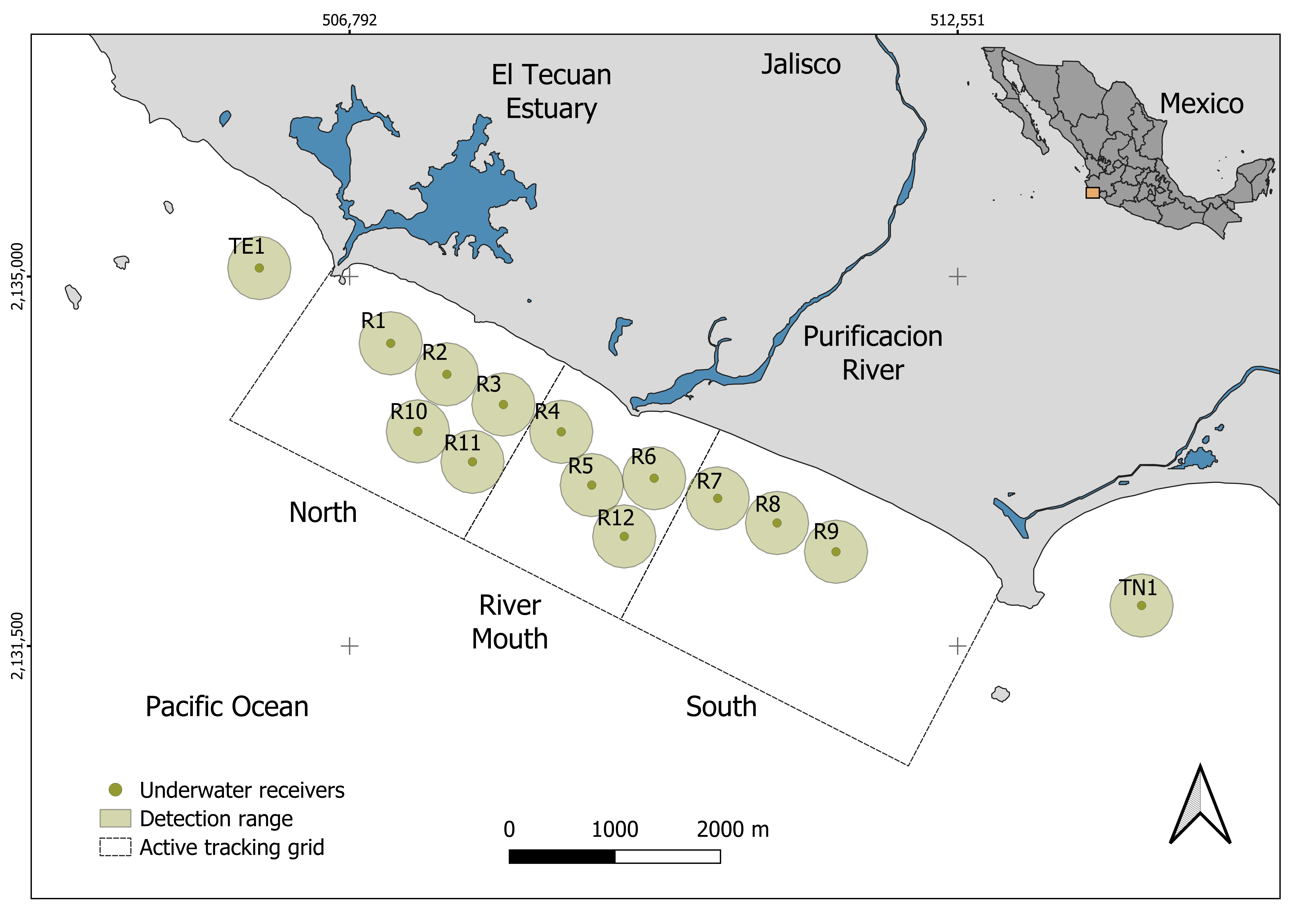
This study was conducted along the southern coast of Jalisco, Mexico, in a 7 km coast stretch known as the Rebalsito area (Figure 1). This high-energy beach is characterized by the mouth of the Purificación River in its central section. Physically, the benthic habitat is characterized by a predominantly soft sandy–muddy bottom. However, structural complexity increases at both ends of the study area and in the central section directly opposite the river mouth, where rocky outcrops are present [25].

The study area has a seasonal hydroclimatic pattern consisting of three periods: mixed (February to May), with cool (<25 °C) and saline waters due to coastal upwelling and lack of rainfall; stratified (July to November), characterized by tropical conditions, rainy and hurricane season, elevated temperatures (>28 °C), and lower salinity waters; and semi-mixed (December, January, and June), which is a transition with intermediate levels [21]. During the rainy season, significant freshwater input from the river creates distinct physicochemical conditions, influencing the local marine habitat. For analysis, the study area was divided into three zones: North (2.4 km to the north of the River Mouth zone), River Mouth (an 800 m radius around the river mouth), and South (the 3 km south of the River Mouth zone), extending approximately 2 km offshore.

An array of underwater acoustic receivers (VR2W, VEMCO-InnovaSea, Bedford, QC, Canada; 390-m detection radius [25]) was deployed in the Rebalsito area. Array coverage expanded across three annual sampling seasons (S1: 2014 to S3: 2016), increasing from six (~2.8 km²) to twelve receivers (~5.7 km²). Receivers were positioned at depths ranging from 10 m to 27 m, with two units placed outside the study area in S3 (Figure 1). Passive tracking was complemented by weekly active tracking using a systematic 800 m grid survey [21].

2.2. Shark Capture and Tagging

Young-of-the-year scalloped hammerheads were captured using a 30-hook bottom long-line [21]. Biological data were collected from each shark, including total length (TL, cm), weight (g), sex, and umbilical scar status (unhealed/well-healed), which was used to classify neonates (less than 15 days old) and non-neonates following Duncan and Holland [19]. All sharks used in this study were externally tagged with a T-bar anchor tag (FD-94, Floy Tag, Seattle, DC, USA) at the base of the first dorsal fin and with ultrasonic transmitters (VEMCO-InnovaSea, Bedford, QC, Canada) to monitor residency and space use. To prevent acoustic signal collisions, most individuals were fitted with V9 transmitters (VEMCO-InnovaSea, Bedford, QC, Canada) programmed with a random repeat interval range of 30–90 s, yielding an expected battery life range of 221–259 days. Additionally, two individuals received V9A transmitters operating at a 15–45 s random repeat interval range, with an estimated battery life of ~36 days. The entire capture, data collection, and tagging procedure was designed to minimize handling time and associated stress [21], with the weight of the acoustic transmitter never exceeding 2% of the shark’s body weight, following established animal welfare guidelines [31].

2.3. Environmental and Biological Variables

We modeled the spatial distribution of S. lewini using a suite of environmental and biological predictors, including total length (TL, cm), weight (W, g), sex, and the relative condition factor (Kn). Kn was calculated as the ratio of the observed weight to the expected weight (Kn = W_obs/W_pred) [32], using a local length–weight relationship for YOY S. lewini [33].

Environmental predictors were sourced as follows: sea surface temperature (SST, °C), and data were obtained as daily 4 km satellite resolution products from the NASA OceanColor Web portal [34]. Gaps in the satellite data due to cloud cover were filled using linear interpolation independently for each season. To minimize the bias of single-pixel interpolation across cloud gaps, daily SST values were not extracted from a single fixed point. Instead, values were spatially averaged across a bounding box (longitude: −105.067 to −104.818, latitude: 19.218 to 19.393) covering the entire acoustic array and adjacent coastal waters. Given the 4 km resolution, these variables reflect regional coastal oceanographic conditions rather than fine-scale gradients within the river plume itself.

Given the region’s mixed semidiurnal tidal regime, tidal data including Tide Level (mm, relative to mean sea level) and Tide Phase (flood, high tide, ebb, and low tide) were obtained for each minute of the study period via MAR V1.0 software [35]. The suncalc R package (version 0.5.1) was used to calculate sunrise and sunset times for each day, as well as lunar illumination. Based on these times, the Diel phase variable was categorized as dawn (sunrise ± 2 h), day (time between the end of dawn and the start of dusk), dusk (sunset ± 2 h), and night (period between the end of dusk and the start of dawn). Lunar illumination was included as a continuous variable following a cyclic index (0 to 1), where both extremes correspond to minimum luminosity. To distinguish between the rising and setting phases of the cycle, intervals were defined as: new moon (waxing phase, 0 to <0.125), first quarter (≥0.125 to <0.375), full moon (≥0.375 to <0.625), last quarter (≥0.625 to <0.875), and new moon (waning phase, ≥0.875 to ≤1). Accumulated precipitation data over 60 days (Precip, mm) were obtained from local National Commission of Water (CONAGUA) meteorological stations [36]. A 60-day accumulation window was selected to serve as a proxy for the hydrological memory of the watershed. This timeframe captures the sustained cumulative discharge needed to breach the river mouth sandbar, aligning with previously documented two-month lags between the cessation of heavy rainfall and shark emigration from this nursery [21].

2.4. Data Analysis

Data analysis was conducted using R statistical software version 4.4.2 [37], with spatial representation performed in QGIS software version 3.34.15 [38]. The raw detection dataset was filtered to remove duplicate signals recorded by multiple receivers within the same minute. Following this filtering, each remaining record represented a unique shark at a unique location within a given minute.

2.4.1. Home Range Analysis

To quantify space use, we estimated core-use areas (50% contour) and home range (95% contour) using Kernel Utilization Distributions (KUDs) with the adehabitatHR R package (version 0.4.22) [39]. Smoothing parameter (h) was selected using the standard reference bandwidth (h_ref) [40]. Individuals detected on only a single day or with fewer than five distinct locations were excluded from this analysis.

To quantify uncertainty in individual KUD area estimations, 95% confidence intervals (CIs) were obtained via non-parametric bootstrapping (999 replicates) [41]. Due to non-normal distributions and limited sample sizes, group-level variability is reported as ranges (minimum–maximum) or interquartile ranges. A series of KUD analyses was performed to evaluate spatial patterns at multiple biological and environmental levels, including (i) an overall KUD pooling all detections, (ii) seasonal KUDs, (iii) Diel-phase KUDs (dawn, day, dusk, and night), and (iv) KUDs stratified by total length and relative condition (Kn).

For group-level comparisons (season, Diel phase, and lunar phase), KUD areas were analyzed using Kruskal–Wallis tests, followed by Dunn’s post hoc tests for pairwise comparisons. To assess the influence of biological traits, the relationship between KUD area (50% and 95%) and continuous variables (total length and relative condition factor, Kn) were evaluated using Spearman’s rank correlation. Additionally, differences in home range size between body condition classes (Kn < 1.0 vs. Kn ≥ 1.0) were assessed using a Wilcoxon rank sum test.

2.4.2. Modeling

To investigate the factors influencing shark presence and spatial distribution, we developed two separate classification models using the Random Forest algorithm. To ensure a standardized measure of temporal availability and constant hourly effort, these models were trained exclusively using detection data from the fixed passive acoustic array (VR2W receivers), excluding sporadic detections from active boat-based tracking. All models were implemented using the Random Forest algorithm via the caret R package (version 6.0-94) [42] and the randomForest package (version 4.7-1.2) [43]. For each analysis (presence/absence and spatial distribution), the dataset was randomly split into a training set (70%) and testing set (30%). Prior to modeling, predictor collinearity was evaluated independently for each dataset using association metrics adapted for mixed data types (Pearsons r, Cramer’s V, and correlation ratio η). Variable pairs exceeding an association threshold of 0.7 were reviewed, and the predictor considered less ecologically distinct or with lower measurement resolution was excluded to reduce redundancy. In addition, predictors with near-zero variance were excluded to reduce noise and improve model stability.

Model tuning and selection was performed exclusively on the training data using repeated 10-fold cross-validation [44,45]. Given the unbalanced nature of detection data, model performance during cross-validation was primarily evaluated using the area under the precision–recall curve (AUPRC), which provides a more informative measure of discrimination under skewed class prevalence than traditional metrics [44,45]. To avoid overinterpretation of a single optimal solution, we adopted a Rashomon set framework, defined as the set of models achieving near-optimal predictive performance within a given hypothesis space [46]. Following this principle, all Random Forest configurations with cross-validated AUPRC values within 1% of the best-performing model were retained for inference [47]. This ensemble-based strategy allows ecological interpretation to be grounded in a family of comparably accurate models, thereby improving robustness and reducing sensitivity to parameterization [48].

Final model performance was evaluated on the independent test dataset using multiple complementary metrics, including AUPRC, area under the receiver operating characteristic curve (AUC-ROC), and the Brier score. These metrics jointly assess discrimination capacity, performance under class imbalance, and probabilistic calibration [49,50]. Models within the Rashomon set were interpreted collectively to characterize predictor importance and ecological response stability in similarly well-performing solutions. Training metrics are reported for completeness only and were not used for model selection or inference.

Permutation-based variable importance was quantified as the mean decrease in area under the precision–recall curve (AUPRC) following random shuffling of each predictor. Importance was primarily estimated on the training dataset to characterize the contribution of each variable to the learned decision structure of the models, thereby supporting ecological inference. To account for model uncertainty, importance values were aggregated in all models retained within the Rashomon set and summarized using the median and range. As a robustness check, permutation importance was also computed on the independent test dataset, where absolute importance values were expectedly reduced due to lower baseline predictive performance.

For the presence/absence analysis, data were structured at an hourly resolution to assess the factors influencing whether sharks were detected within the monitored area. Artificial absences were generated from hourly intervals without detections to approximate temporal availability. To account for the uneven number of receivers across the study site and avoid spatial effort bias, data aggregation and pseudo-absence generation were conducted at the zone level (North, River Mouth, and South). Specifically, an artificial absence was recorded for a given zone only if a shark was not detected by any receiver within that entire spatial unit during a one-hour period. These pseudo-absences represent non-detections rather than confirmed absences, reflecting a detectability process while effectively standardizing the spatial sampling effort. For the complementary spatial distribution model, detection-only data were used to predict the probability of shark occurrence among these same three predefined zones based on environmental and biological predictors.

Model interpretation relied on two complementary, model-agnostic approaches. Predictor importance was quantified using a permutation-based method (n_sim = 1000) implemented with the vip R package (version 0.4.1) [51], which estimates the mean decrease in predictive performance when individual predictors are randomly permuted [52,53].

To visualize the marginal effects of influential predictors, we used accumulated local effects (ALE) plots for continuous variables and partial dependence plots (PDPs) for categorical predictors. ALE values visualize the effect centered at zero, representing the percentage-point change in probability relative to the average model prediction. These plots included overlaid individual conditional expectation (ICE) curves to assess model consistency. For categorical predictors, PDPs estimated the absolute marginal predicted probability of occurrence; variability was visualized using standard deviation error bars derived from the Rashomon set models, rather than raw ICE curves, to ensure visual clarity. All interpretation plots were generated using the iml R package (version 0.11.4) [54].

3. Results

A total of 20 YOY scalloped hammerhead sharks were tagged with ultrasonic transmitters during the three sampling seasons in the Rebalsito area (

Table 1. Biological characteristics, tagging metadata, and monitoring effort for young-of-the-year (YOY) Sphyrna lewini tracked across three sampling seasons. Kn denotes the relative condition factor. Asterisks (*) indicate individuals excluded from space-use analyses due to sparse detection data.

Season	ID	TL (cm)	Weight (g)	Kn	Sex	Tagging Date	Days Monitored	Days Detected
S1	16,300	70.4	1400	0.90	H	27 October2014	12	7
	16,299	53.7	680	0.93	M	28 October 2014	11	8
	7762	56.2	750	0.90	H	28 October 2014	10	6
	16,304	57.9	910	1.00	M	6 November 2014	52	25
	16,301	63.1	110	0.94	M	24 November 2014	47	27
	16,302 *	72.1	1800	1.08	H	8 December 2014	2	2
	17,491	64.4	1400	1.12	H	8 December 2014	45	14
S2	37,907	76.5	2030	1.01	M	9 November 2015	71	5
	37,908 *	72.6	2160	1.27	H	11 November 2015	70	2
	37,912 *	61.0	1080	1.02	H	23 November 2015	68	1
	37,905	56.1	780	0.94	H	25 November 2015	67	4
	37,913	72.1	1370	0.82	H	2 December 2015	60	10
	37,904	59.1	1030	1.06	H	7 December 2015	55	6
	37,906	65.0	1290	1.00	H	7 December 2015	55	18
	1934	58.4	980	1.05	H	10 December 2015	52	11
	1931 *	57.0	870	1.00	M	10 December 2015	52	1
S3	37,909	55.6	710	0.88	M	24 November 2016	68	9
	42,022	67.3	1110	0.78	H	24 November2016	20	5
	37,910	71.7	1750	1.07	H	5 December 2016	57	9
	37,911	55.8	730	0.89	M	5 December 2016	57	2

): seven in S1, nine in S2, and four in S3. All individuals were captured and tagged between October and December of each season. Total length (TL) was in the range of 53.7–76.5 cm (mean ± SD: 63.3 ± 7.2 cm) and weighed in the range of 680–2160 g (mean ± SD: 1197 ± 447 g). The relative condition factor (Kn) varied considerably among individuals (range: 0.78–1.27; mean ± SD: 0.98 ± 0.11), with 55% of the sharks exhibiting high condition (Kn ≥ 1, n = 11) and 45% showing low condition (Kn < 1, n = 9). The sex ratio of the sharks included in the analysis was F:M = 1:0.60. The transmitter-to-body mass ratio never exceeded 0.82%. One shark from S1 and three from S2 were excluded from space-use analyses because they were detected on only a single day or had fewer than five distinct locations.

3.1. General Detection Patterns

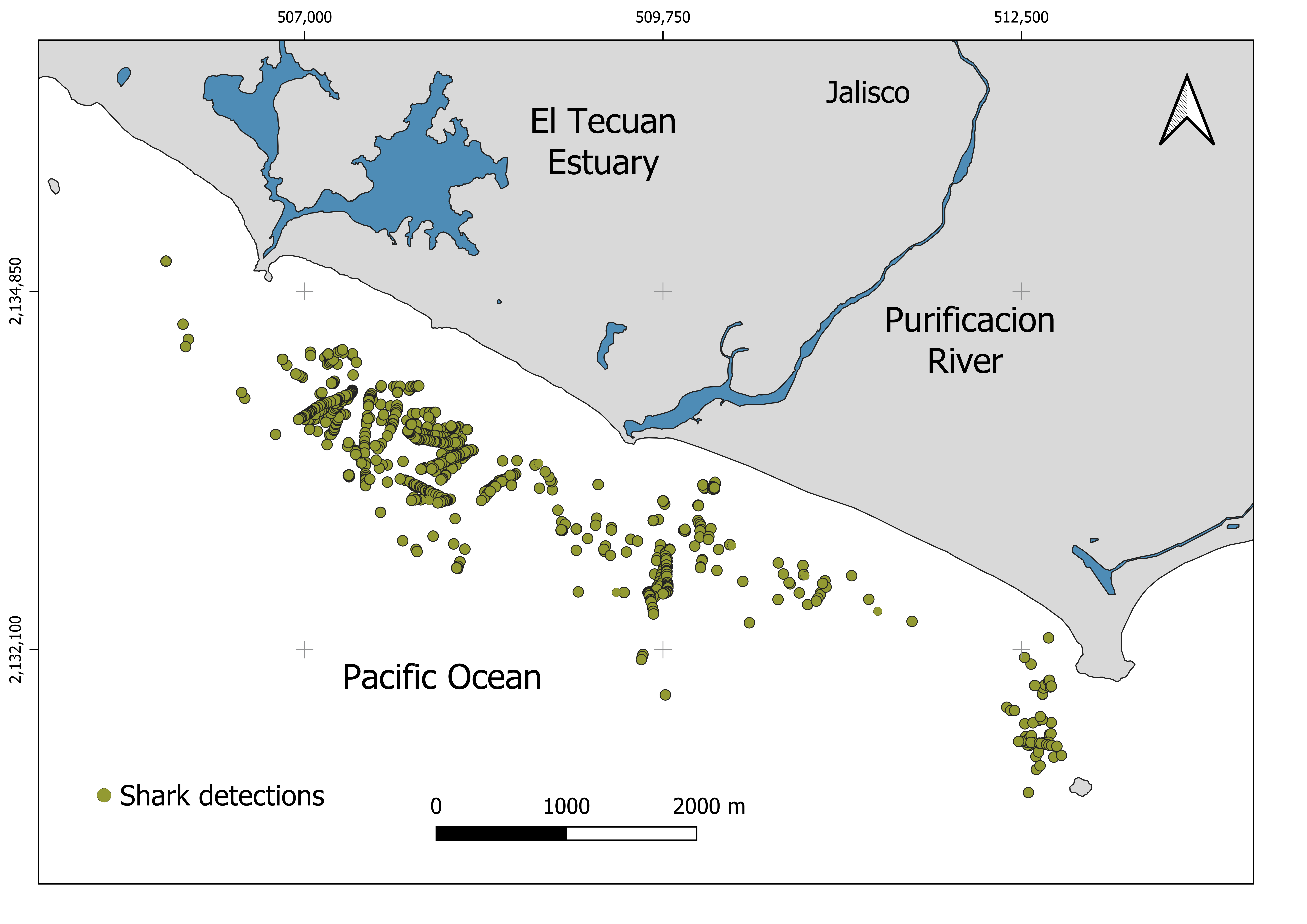
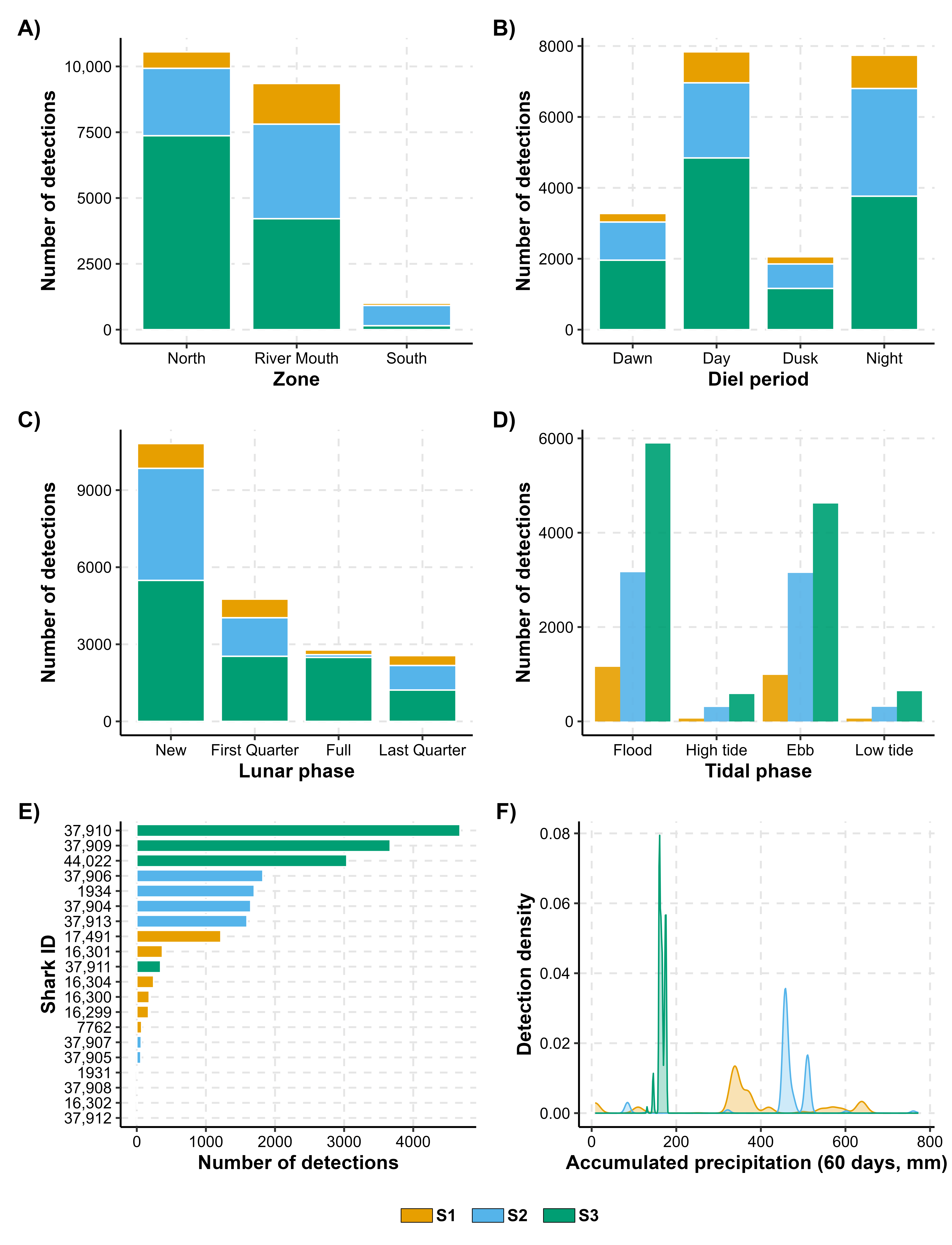
Across the three seasons, a total of 20,910 detections were recorded (Figure 2), with sharks tagged in S1, S2, and S3 contributing 10.8%, 33.1%, and 56.1% of the dataset, respectively. Detection frequency varied substantially among sharks, ranging from 3 to 4677 detections per individual (median: 294 detections).

The temporal span of detections was strictly seasonal. In S1, tagged sharks were detected between 27 October 2014 and 21 January 2015; in S2, between 9 November 2015 and 6 January 2016; and in S3, from 24 November 2016 to 14 December 2016. Crucially, no further detections were recorded after these dates, even though the acoustic array remained fully operational for several subsequent months.

Spatially, detections were most frequent in the North zone of the study area (10,555 detections, 50.5%), where 19 sharks were recorded (Figure 3). The River Mouth accounted for 9351 detections (44.7%, 17 sharks), while the South zone had 1004 detections (4.8%, 11 sharks). Considering the Diel phase, the detections recorded were: dawn (2321 detections, 11.1%), day (6183; 29.6%), dusk (4947; 23.7%), and night (7450; 35.6%).

Environmental conditions also exhibited substantial variability throughout the study period, and several of these factors were associated with clear differences in detection frequency. Lunar illumination showed the strongest differences, with detections peaking during the darkest conditions (new moon: 10,812 detections), followed by first quarter (4759), full moon (2780), and last quarter (2560) (Figure 3C). A similar pattern emerged for tidal stage where most detections occurred during dynamic tidal phases—flood (10,209) and ebb (8747)—whereas high and low tide yielded markedly fewer detections (944 and 1011, respectively), a trend consistent among seasons. Longer-term hydroclimatic conditions also varied widely among seasons. Accumulated precipitation ranged from 8.2 to 671.1 mm in S1, 84.4 to 772.5 mm in S2, and 86.8 to 174.9 mm in S3, with detection density increasing when accumulated precipitation exceeded ~100 mm (Figure 3F).

3.2. Home Range

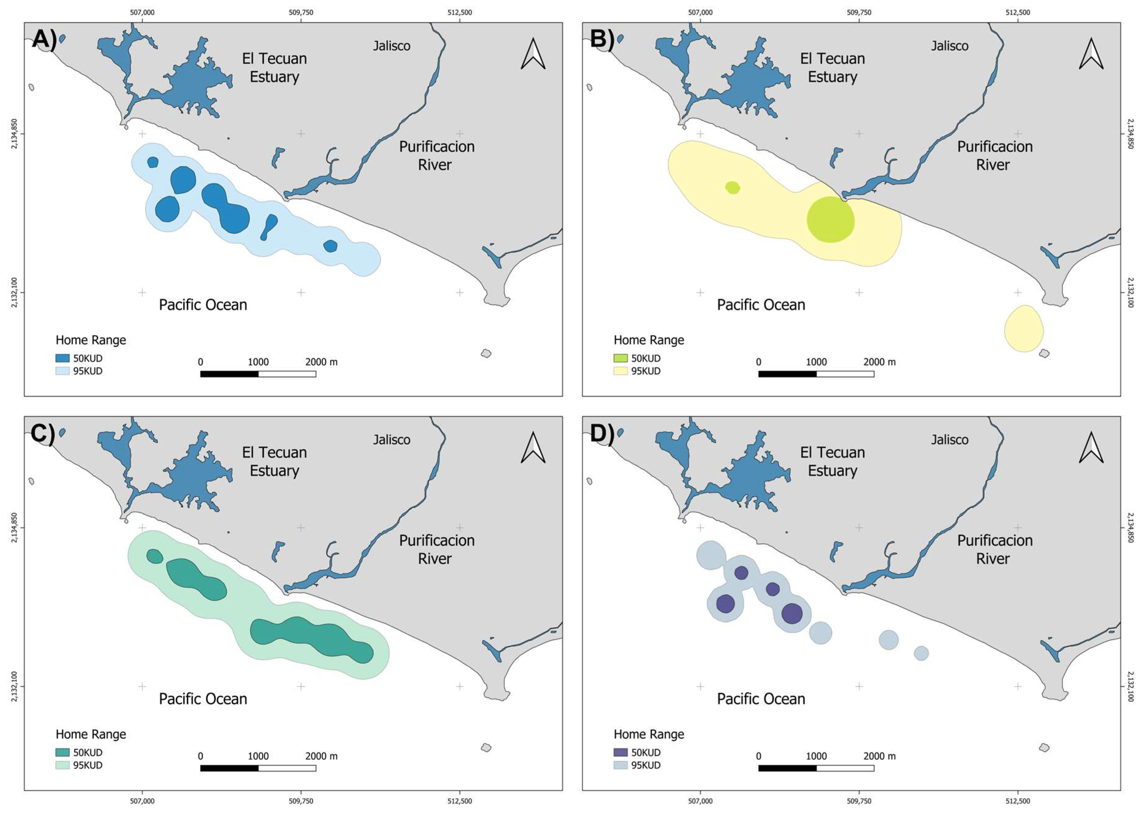
Pooling all detections during the study period, sharks exhibited a core use area of 0.86 km² (50%KUD, 95% CI: 0.83–0.87) and a broader home range of 3.52 km² (95%KUD, 95% CI: 3.46–3.57; Table S1). Space use was primarily concentrated in front of the river mouth and in the northern sector of the study area (Figure 4A).

Marked seasonal variation in space use was evident (Figure 4B–D). The largest core area occurred during S2 (1.28 km²; 95% CI: 1.26–1.33), nearly double that observed in S1 (0.59 km²; 95% CI: 0.53–0.69) and exceeding by fivefold the highly restricted area used in S3 (0.26 km²; 95% CI: 0.25–0.28), when detections were largely confined to the northern zone. These patterns indicate pronounced temporal shifts in spatial behavior despite shared nursery habitat.

Space use also varied among Diel cycles. Based on individual home range estimations, sharks utilized the largest median core areas and home range during crepuscular periods (dawn: 4.65 km²; dusk: 4.64 km²) and night (4.17 km²), whereas spatial use was notably more restricted during the day (3.06 km²; Table S2). However, due to high individual variability, these differences were not statistically significant (Kruskal–Wallis: χ² = 1.193, df = 3, p = 0.755). This pattern suggests an expansion of movements during low-light periods compared to daytime hours

Lunar illumination further influenced space use. Median core areas (50% KUD) were smallest during new moon (0.43 km²) and last quarter (0.48 km²) phases, remaining relatively low during the first quarter (0.50 km²) but showing a notable increase during full moon conditions (1.09 km², Table S2). A similar trend was observed for home ranges (95%KUD), with the most restricted movements occurring during first quarter (2.51 km²), last quarter (2.64 km²), and new moon (2.93 km²) phases, while full moon periods prompted a substantial expansion in habitat use (5.30 km²). However, despite these trends, the differences were not statistically significant (Kruskal–Wallis: χ² = 2.027, df = 3, p = 0.567), likely due to high individual heterogeneity. It is worth noting that while the median home range was lowest in the first quarter, this phase also exhibited the widest range of variability [1.16–26.21 km²] driven by extreme individual movements.

Although larger sharks (≥70 cm TL) displayed visually larger core-use areas (50% KUD: 1.09 km²) and home ranges (95% KUD: 4.82 km²) compared to smaller individuals (<70 cm TL, 0.97 km² and 4.46 km², respectively; Table S2), these differences were not statistically significant (Wilcoxon rank sum test: W = 16, p = 0.36). Furthermore, total length showed no monotonic association with either the 50% KUD (Spearman: ρ = −0.005, p = 0.986) or the 95% KUD (Spearman: ρ = −0.027, p = 0.929). However, this result should be interpreted cautiously because three of the larger sharks (>70 cm TL; IDs 16,302, 37,907, and 37,908) were detected only 7, 33, and 12 times, respectively, during more than one day and largely within the same area. This limited spatial spread in detections likely led to an underestimation of their KUDs, particularly if these individuals used portions of their home range beyond the receiver array.

Similarly, the relative condition factor (Kn) did not show a statistically significant influence on the spatial extent of habitat use. Although initial aggregated estimates suggested larger areas for individuals with high body condition (Kn ≥ 1.0), the analysis of individual home ranges revealed that these differences were driven by high individual variability rather than a consistent biological pattern (Wilcoxon rank sum test: W = 38, p = 0.54). The median home range size was remarkably similar between groups: 4.63 km² (range: 0.93–24.60 km², Table S2) for individuals with lower condition (Kn < 1.0) and 4.53 km² (range: 0.19–5.59 km²) for those with higher condition (Kn ≥ 1.0). The wider range observed in the lower-condition group is largely driven by a single individual (ID 16,300) with an exceptionally large home range (24.6 km²).

3.3. Shark Presence

The final dataset evaluated by the presence/absence model comprised 1500 presence records and 10,709 pseudo-absence records, yielding a presence-to-pseudo-absence ratio of approximately 1:7.1 (12.3% presences). Within this dataset, no predictors exhibited zero variance, and no pairwise correlations exceeded the collinearity threshold (>0.7), indicating that all retained predictors contributed non-redundant information to the model. The final set of predictors included season, lunar illumination, accumulated precipitation (60 days), sea surface temperature (SST), Diel phase, tide phase, and tide level. Biological variables (TL, Kn) were excluded from this model because they are conditional on shark detection. Consequently, their influence was only evaluated in the spatial distribution model to explain movements between zones.

Cross-validation identified the model configured with mtry = 2 as the top-performing configuration (AUPRC = 0.5263). One additional model (mtry = 3) achieved performance within 1% of this value (AUPRC = 0.5260) and was therefore included in the Rashomon set for comparative interpretation (

Table 2. Summary of predictive performance on the independent test dataset for the Random Forest models retained in the Rashomon set. Values indicate the range (minimum–maximum) of performance metrics observed across the selected models for both presence/absence (mtry 2, 3) and spatial distribution (mtry 6 to 10) analyses. Model selection was based on the cross-validated area under the precision–recall curve (AUPRC). Threshold-dependent metrics (sensitivity and specificity) were calculated using a fixed probability threshold of 0.5.

Model Type	Rashomon Models (mtry)	AUPRC	AUC-ROC	Sensitivity	Specificity	Brier Score
Presence/Absence	2, 3	0.474–0.479	0.870–0.873	0.30–0.37	0.96–0.97	0.086–0.088
Spatial Distribution	6–10	0.978–0.984	0.987–0.991	>0.96 *	>0.99 *	0.043–0.061

* Sensitivity and specificity for the spatial distribution model vary by zone; reported values correspond to the highest-performing zones (North and River Mouth). See Table S6 for detailed class-wise metrics.

and Table S3).

When evaluated on the independent test dataset, the two retained models exhibited consistent discriminatory ability (AUC-ROC = 0.870–0.873), and moderate precision under class imbalance (AUPRC = 0.474–0.479). The Brier scores were low (0.0855–0.0879), indicating good calibration and predicted probabilities.

Specificity remained high (>0.95), whereas sensitivity was more moderate (0.304–0.371; Table 2 and Table S3), reflecting a conservative classification behavior that prioritizes reducing false positives in a system characterized by relatively infrequent detections.

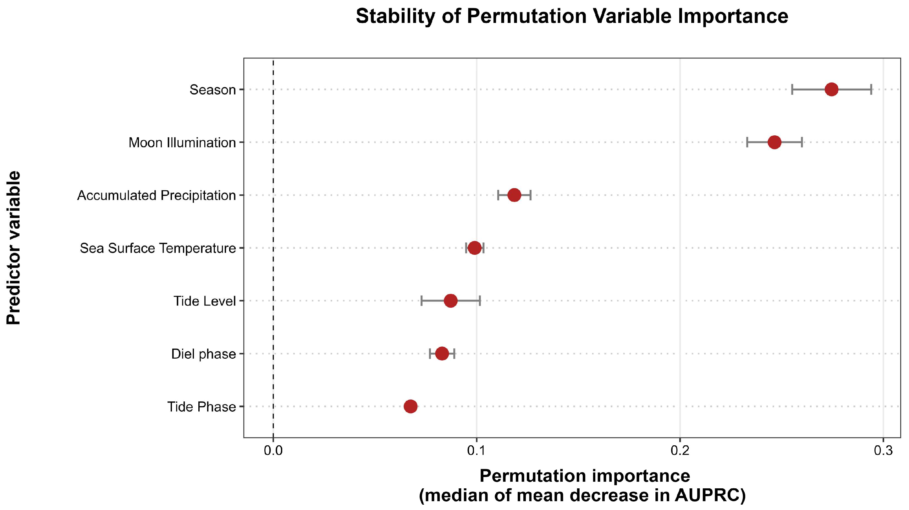
Permutation-based importance analysis identified a clear hierarchy of predictors in the Rashomon set (Figure 5, Table S4). Season emerged as the dominant driver of shark presence, showing the largest median permutation importance (median decrease AUPRC (MDPR) = 0.276, range: 0.258 −0.294), followed closely by moon illumination (median MDPR = 0.247, range: 0.234–0.260).

A second group of predictors exhibited consistently positive but substantially lower contributions to model performance. Within this group, accumulated precipitation was the most influential variable (median MDPR = 0.118), followed by sea surface temperature (median MDPR = 0.100), tide level (MDPR = 0.089), Diel phase (median MDPR = 0.084), and tide phase (MDPR = 0.069, Figure 5). The permutation importance values of these predictors (lower than season and lunar illumination) indicate a secondary role in shaping shark presence at the temporal scale analyzed.

Despite the variability in detection numbers among individuals and seasons, the Rashomon set analysis revealed high stability in variable importance ranking (Figure 5). The narrow range of permutation importance values for environmental predictors across the set of near-optimal models confirms that the identified drivers are robust to data subsampling and parameter perturbations, reducing the likelihood that results are driven by a few hyper-abundant individuals in S3.

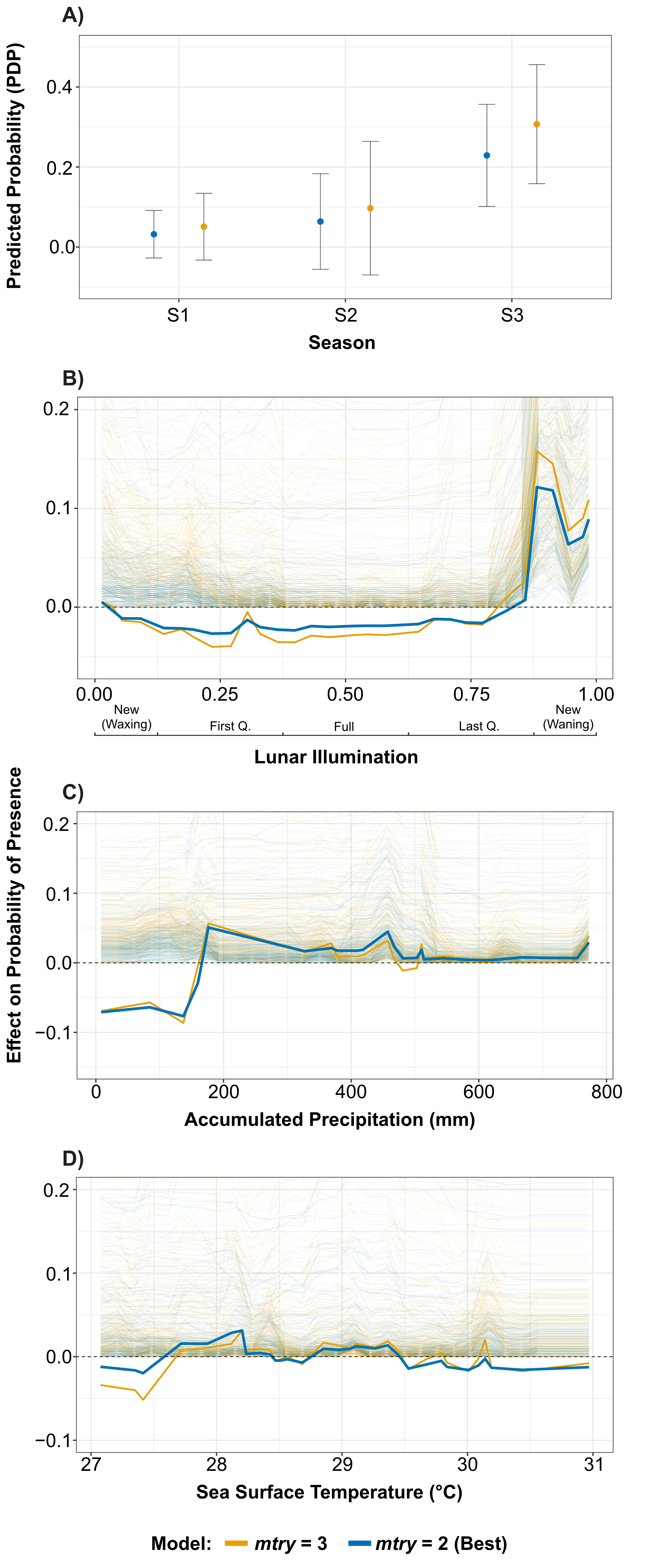
Season was the strongest predictor of shark presence, showing consistent effects in all Random Forest models (Figure 6A). Interpreted via PDP, which represent the absolute predicted probability of occurrence, season S3 exhibited the highest occupancy, with a mean probability of 0.27 (±0.14 SD). In contrast, S1 showed the lowest probability (0.04 ± 0.07 SD), indicating a clear seasonal gradient in habitat use.

Lunar Illumination showed a strong and non-linear influence on shark presence (Figure 6B). ALE curves remained close to zero or slightly negative during most of the lunar cycle, but increased sharply as the index approached 0.875–1.0, corresponding to the new moon waning phase category. During this specific window, positive effects reached approximately 0.12–0.15 percentage points above the model average. This pattern indicates a higher predicted probability of presence during the darkest nights occurring at the end of the lunar cycle, whereas the new moon waxing phase window (start of the cycle) was associated with neutral or negative effects. In contrast, values around the range of 0.375–0.625 (full-moon) were associated with near-zero or lower effects relative to the model baseline. This pattern was consistent in all models in the Rashomon set, supporting a robust lunar cycle signal.

Accumulated precipitation over 60 days showed a non-linear, threshold-like effect on shark presence (Figure 6C). At low precipitation levels (<100 mm), ALE values were predominantly negative (down to −0.09), indicating reduced presence probability. In contrast, precipitation near or slightly exceeding 200 mm resulted in positive effects in the range of 0.05–0.06, while higher values (up to 600 mm) clustered around zero. This pattern suggests that prolonged rainfall enhances habitat suitability only beyond a minimum accumulation threshold.

Sea surface temperature (SST) exhibited comparatively weak and irregular effects on shark presence (Figure 6D). ALE curves showed modest positive deviations (≤0.03) around 28 °C and 30 °C. Probabilities reached negative values (−0.05) for temperatures below 27.5 °C. High dispersion in the ICE curves indicates substantial inter-individual and context-dependent variability suggesting that SST alone explains little variation in presence probability and likely acts as a secondary or interacting driver rather than a primary determinant.

3.4. Spatial Distribution

For the dataset used to model spatial distribution, no predictors were identified with zero variance. Correlation analysis revealed strong collinearity between total length (TL) and weight (r = 0.901, p < 0.001); therefore, weight was excluded from subsequent analyses. Although seasonal and hydroclimatic variables (precipitation, SST) showed moderate-to-high association (η > 0.7), all were initially retained to allow the Random Forest algorithm to resolve variable importance based on hierarchical predictive power.

The spatial distribution model showed excellent predictive performance under a multiclass framework. The best-performing configuration (mtry = 10) achieved a cross-validated macro-AUPRC of 0.988 and AUC-ROC of 0.995, together with a low Brier score (0.043), indicating both strong discrimination and good probability calibration (Table 2). Classification accuracy was also high, with macro-average F1-scores and balanced accuracy on the independent test dataset exceeding 0.96 (Table S5).

Model stability was high across the tuning space. Configurations with mtry values between 6 and 10 fell within 1% of the best cross-validated macro-AUPRC and were therefore retained in the Rashomon set. Performance variability across these models was minimal (test macro-AUPRC = 0.982–0.988; Brier score = 0.043–0.061), indicating that spatial predictions were robust to model parameterization.

Class-wise performance metrics revealed high predictive accuracy for all spatial zones, with consistent patterns observed among the models retained in the Rashomon set (Table S6). For the best-performing configurations (e.g., mtry = 10), sensitivity was particularly high for the North and River Mouth zones (recall > 0.96, in the independent test set), indicating robust classification performance and stable spatial assignment within these areas. Although sensitivity for the South zone was comparatively lower (0.83–0.93), its consistently high specificity (>0.99) across optimal configurations reflects a robust discrimination power). This pattern indicates greater spatiotemporal variability, characteristic of transient rather than resident behavior within the South zone. Conversely, the higher and more stable performance observed for the North and River Mouth zones aligns with their roles as core habitat areas with more persistent occupancy patterns.

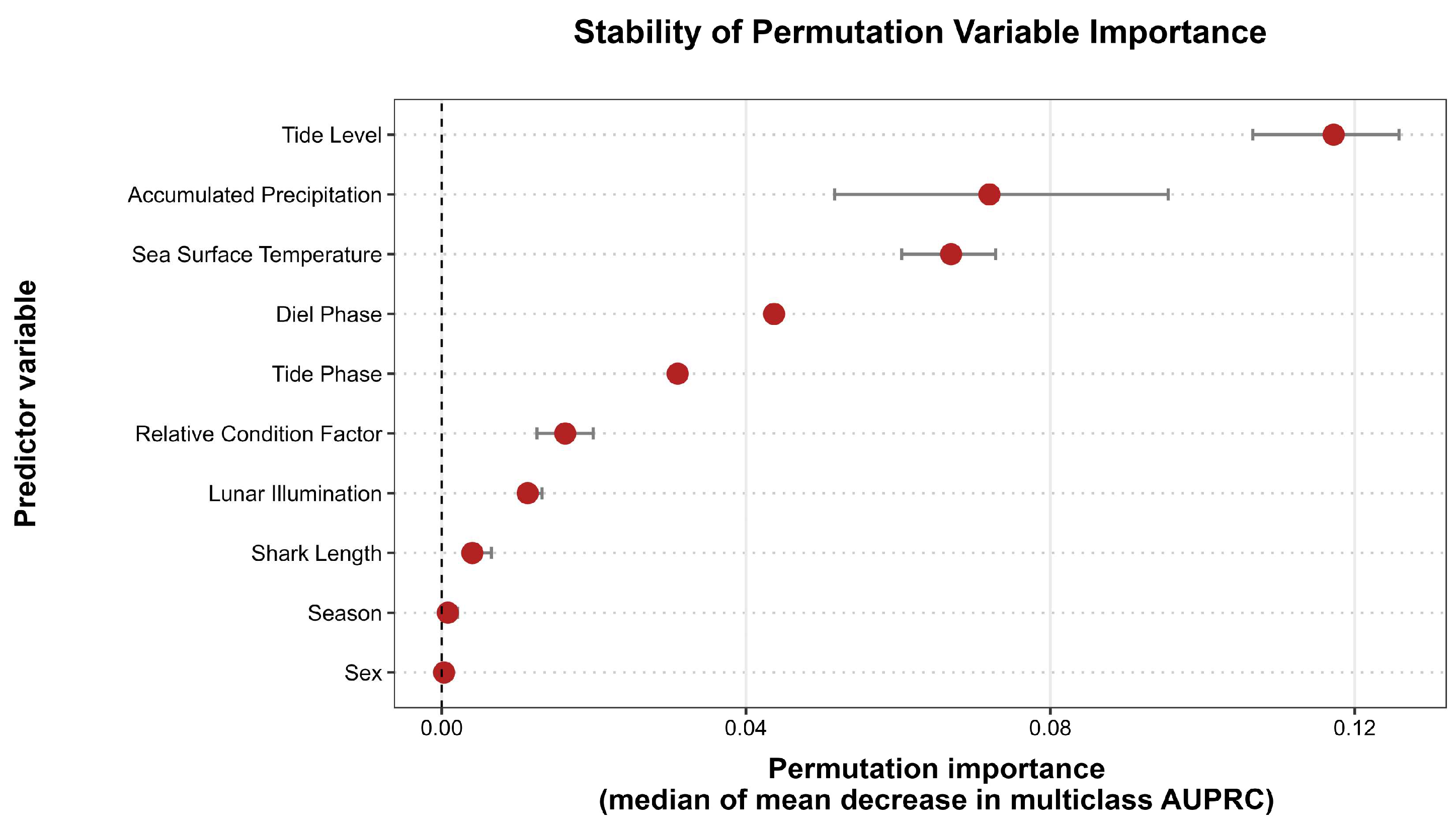
Permutation-based importance analysis for the spatial distribution model identified a hierarchy among predictor variables (Figure 7, Table S7). Tide level was the most influential predictor (median MDPR = 0.117), exhibiting a narrow importance range across the Rashomon set (0.107–0.126), which indicates a consistently strong and robust effect on spatial zone selection.

Regarding tidal dynamics, although tide phase held substantially lower importance (median MDPR = 0.031), the correlation between tide level and tide phase was low (η = 0.35, p < 0.001). This statistical independence confirms that phase provides complementary hydrodynamic information; therefore, both were retained to fully characterize the tidal forcing.

Accumulated precipitation (60 days) ranked second in importance (median MDPR = 0.072) but displayed the widest importance range (0.052–0.095). This contrast suggests that while tidal influence is stable, rainfall acts as a context-dependent driver whose influence varies across near-optimal model configurations. Sea surface temperature completed the trio of top predictors, exhibiting moderate importance (median MDPR = 0.067) with limited cross-model variability, supporting a secondary but consistent role in spatial distribution.

Following these primary drivers, the Diel phase showed intermediate influence (median MDPR = 0.043). The hierarchy was completed by a final cluster of lower-ranking but relevant variables: the relative condition factor (Kn), the most relevant biological predictor (median MDPR = 0.016), and lunar illumination (median MDPR = 0.011). In contrast, shark length, season, and sex consistently yielded near-zero importance values, confirming their negligible contribution to explaining fine-scale spatial distribution patterns in the final model.

Notably, importance values in the independent test dataset closely mirrored those in the training set (Table S7), confirming the high generalization capability of the model regarding these primary drivers.

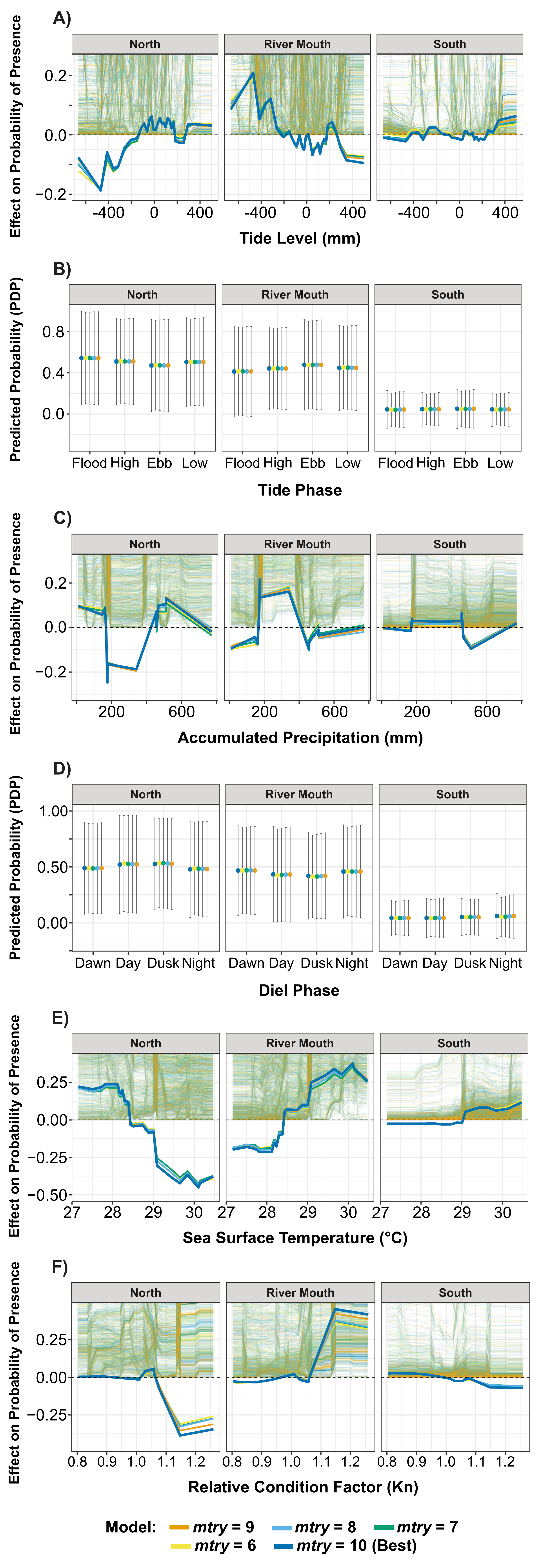
Model-averaged accumulated local effect (ALE) plots and partial dependence plots (PDPs) revealed distinct and ecologically interpretable spatial responses to the most influential predictors (Figure 8).

Tide level exerted the strongest and most consistent influence on spatial distribution (Figure 8A). Under very low tide conditions (approximately −600 to −450 mm), the probability of occupancy decreased markedly in the North zone (effects of ~−0.15 to −0.20), while simultaneously increasing in the River Mouth (up to ~+0.18 to +0.22). As tide level rose toward intermediate values (~−250 to 0 mm), North effects approached zero and became slightly positive, whereas River Mouth effects declined to near-zero and turned negative at higher tide levels (down to ~−0.05 to −0.10). The South zone remained weakly structured by tide levels overall but showed a small increase in preference under higher tide levels (>~250–300 mm).

Consistent with this pattern, the tide phase (PDP, Figure 8B) corroborated a hydrodynamic partitioning. The River Mouth showed higher occupancy probabilities during ebb (0.48 ± 0.43 SD) and low tide (0.45 ± 0.41 SD), matching the preference for receding water levels. In contrast, the North zone exhibited peak probabilities during flood (0.54 ± 0.45 SD), suggesting a spatial displacement driven by tidal flow direction. Meanwhile, the South zone maintained consistently low occupancy probabilities (~0.04–0.05) regardless of the tidal phase.

Accumulated precipitation over 60 days showed a strong and highly non-linear influence on spatial distribution, with contrasting responses among zones (Figure 8C). North zone occupancy increased at both low (<200 mm) and high (>350 mm) precipitation levels, but declined at intermediate values. Conversely, the River Mouth exhibited a strong positive response exclusively to moderate precipitation (~200–350 mm), dropping abruptly beyond 400 mm. The South zone displayed a comparatively weak response, mainly characterized by a negative peak deviation at precipitations > 400 mm (~−0.10).

The Diel phase (PDP, Figure 8D) reveals a distinct temporal segregation between zones. The North zone exhibited peak occupancy probabilities during illuminated hours and the evening transition, specifically at day (0.53 ± 0.43 SD) and dusk (0.53 ± 0.40 SD). In contrast, the River Mouth was favored during low-light intervals, showing the highest probabilities at dawn (0.47 ± 0.39 SD) and night (0.46 ± 0.41 SD). Mirroring the trend observed for tidal phase, the South zone displayed negligible variation, maintaining consistently low occupancy probabilities (<0.06) across the entire diel cycle.

Sea surface temperature (SST) showed a pronounced thermal threshold (Figure 8E). In the North zone, cooler conditions (≈ 27.0–28.2 °C) were favored (+0.20 to +0.25), but effects declined sharply as SST approached ~29 °C. The River Mouth exhibited an opposite response: low SST values were associated with negative effects, whereas occupancy increased rapidly between ~28.5 and 29.5 °C, reaching peak positive effects (+0.30 to +0.37). The South zone showed a gradual increase toward positive values above ~29 °C (+0.10 to +0.12).

Finally, the relative condition factor (Kn) displayed a distinct pattern of spatial segregation (Figure 8F). Individuals with superior body condition (Kn > 1.0) were strongly associated with the River Mouth, showing increasing positive effects as condition improved. Conversely, sharks with lower condition indices (Kn < 1.0) were more frequently associated with the North and South zones, where ALE effects were positive for thinner individuals and decreased as body condition improved.

4. Discussion

Understanding the factors that shape the spatial ecology of young-of-the-year sharks is fundamental for identifying the processes that sustain coastal nurseries and for informing conservation strategies. In this study, we show that the fine-scale spatial distribution of YOY Sphyrna lewini along the southern coast of Jalisco is governed by a hierarchy of environmental and biological drivers operating at distinct scales. While broad temporal windows (season and lunar illumination) regulate the overall presence in the nursery, fine-scale spatial partitioning is driven by hydrodynamic conditions (tide, precipitation) and biological traits (size, body condition).

4.1. Environmental Drivers of Presence and Distribution

The spatial ecology of S. lewini during its early life stages is a manifestation of complex trade-offs between foraging optimization and mortality risk mitigation [55,56]. Computational modeling of YOY S. lewini presence consistently identified season and lunar illumination as the strongest environmental predictors of nursery occupancy. In this context, season functions as a proxy for unmeasured oceanographic variability (e.g., current shifts or river mouth dynamics) and resource pulses [18,56].

A key finding of this study is the specific response to lunar illumination. Unlike studies in other Pacific regions reporting aggregations of subadult and adult S. lewini during periods of high lunar illumination, potentially associated with resting refuges or predator avoidance [55,57], YOY S. lewini in Jalisco exhibited a robust preference for the darkest phases of the lunar cycle, specifically the waning new moon (late last quarter phase to new moon). This preference suggests a risk-minimization strategy in an open-coast environment lacking structural refuges, where darkness reduces visual detection by predators [58,59]. Furthermore, this phase correlates with higher vertical migrations of mesopelagic prey [59,60], potentially maximizing foraging efficiency under the cover of darkness [58,59].

Regarding spatial distribution, tide level and precipitation served as the primary modulators of zone-specific occurrence. Unlike other systems, the study area lacks intertidal or sheltered zones that become accessible during high tides, as the entire coastline is directly exposed to open-ocean conditions. Nevertheless, tide level appears to act as a modulator of space use, with sharks concentrating toward the river mouth during low tide. This pattern suggests that the Purificación River plume functions as a dynamic environmental cage, in which turbidity generated by moderate accumulated precipitation (200–350 mm) provides optimal habitat conditions for neonates. Similar patterns have been reported in estuarine systems in Australia [61] and Hawai’i [62], where turbidity is a primary driver of juvenile hammerhead abundance. The ecological importance of turbid plumes in providing refuge and enhancing prey availability is widely acknowledged in coastal nurseries [61,63,64]. Turbidity may be especially advantageous given the enhanced electrosensory and olfactory capabilities of S. lewini [64,65,66], allowing them to forage effectively where visual predators cannot. However, the system showed a tipping point: extreme rainfall (>400–600 mm) triggered a displacement to peripheral zones (North/South), confirming that while freshwater input defines habitat suitability, excessive discharge exceeds the physiological or physical tolerance of the YOY S. lewini. Specifically, extreme river outflow can induce severe osmotic stress due to sudden, drastic drops in coastal salinity, while simultaneously increasing the energetic costs associated with swimming against strong, turbulent currents [11,13,67].

Sea surface temperature also appears to play a role in regulating nursery occupancy. The decline in shark presence coincided with the onset of temperatures below ~27 °C, typically recorded from December onward, suggesting a potential thermal constraint on habitat use. Similar temperature-driven departures from nursery areas have been documented in Carcharhinus plumbeus, which abandons nursery bays along the eastern United States coast when water temperatures fall below 15.9 °C [18]. Likewise, young-of-the-year Carcharhinus leucas disappear from estuarine systems at temperatures below 27.9 °C, while older juveniles can persist under cooler conditions [68]. Crucially, in our study area, this thermal decline coincides with the seasonal closure of the river mouth [21]. This physical closure not only alters hydrodynamics but prevents the export of terrestrial nutrients and reduces estuarine prey availability, acting as a synergistic constraint. Thus, while temperature acts as a physiological cue, the cessation of nutrient input and the physical collapse of the turbidity cage likely function as the ultimate drivers triggering abandonment of the nursery area [18,68].

4.2. Biological Drivers

Our results reveal an ontogenetic spatial segregation driven not only by total length but also by body condition (Kn). The River Mouth functioned as the core habitat for the smallest individuals (<60–65 cm TL) and those with higher relative condition factors (Kn > 1.0). In contrast, larger individuals and those with lower Kn were associated with the North zone. While body condition influences where they are (spatial zone selection), it does not seemingly dictate how much space they use (home range size), as seen in our KUD analysis. This pattern should not be interpreted as unfit individuals being pushed to the periphery. Rather, given the negative allometry of YOY S. lewini growth (b < 3.0) [33], where individuals grow in length faster than in mass, lower Kn values are characteristic of older YOY entering a transitional phase. This spatial shift likely reflects an ontogenetic change in dietary requirements. Stable isotope and stomach content analyses for this species indicate a transition from easy-to-capture, low-energy prey favored by neonates in the river mouth, to higher-energy teleost and rays found in deeper coastal waters [24,69,70]

Consequently, the North zone appears to function as a foraging ground for these transitional juveniles. It is noteworthy that these larger individuals preferentially used a predominantly soft-bottom area in the North rather than adjacent rocky reefs. This avoidance of complex rocky habitats, despite their potential richness, may reflect a strategy to minimize competition with reef-associated predators or simply an exploratory shift to locate energetically more profitable prey.

4.3. Space Use and Home Range

Young-of-the-year S. lewini exhibit a constrained median home range (95% KUD) of 3.52 km². This spatial footprint is representative of the early life-history requirements of a species balancing rapid neonatal growth with predation risk in an open coastal environment [16,71,72].

The home range estimated here is significantly smaller than that reported for YOY pigeye shark (Carcharhinus amboinensis, 63–82 cm TL) in Cleveland Bay, Australia (median = 14.17 km²; range: 0.01–180.53 km²) [73]), a difference likely attributable to the extensive shallow mudflats in Cleveland Bay that facilitate broader movements. Conversely, the home range in Jalisco is larger than estimates for YOY S. lewini (47.8–65 cm TL) in restrictive, semi-enclosed systems like Kāne‘ohe Bay, Hawaii (~1.3 km², range: 0.46–3.52 km² [20,74]) or Negaprion brevirostris in insular lagoons like Los Roques, Venezuela (0.42 ± 0.12 km², 64.5–71.1 cm TL [75]).

This intermediate spatial scale highlights the unique nature of the Purificación River mouth. Unlike mangrove-fringed nurseries that offer structural refugia [76], this open-coast system relies on environmental refugia, specifically the low-visibility conditions provided by the river plume, to minimize predation risk and enhance foraging on estuarine prey [21,64]. Because these boundaries are defined by dynamic turbidity fronts rather than physical walls, sharks exhibit a dynamic residency, constantly adjusting their position to remain within optimal turbidity patches as they shift with tides and river flow [73,77].

While activity was continuous, the contraction of home range observed during the day, contrasted with expansions during crepuscular (dawn, dusk) and nocturnal periods, mirrors the pulsing behavior documented in Kāne‘ohe Bay, where sharks forage widely at night and return to a core area by day [74]. This expansion aligns with meta-analyses indicating that increased horizontal movement during crepuscular periods is a widespread strategy in elasmobranchs to optimize foraging opportunities [78].

Although no linear relation was found between body size and KUD, the detection patterns of the largest YOY size class (70–75 cm TL) suggests an impending ontogenetic shift. These individuals showed sporadic detections over wide temporal window, a pattern likely representing a transitional stage of bathymetric segregation. Rather than a full migration to the continental shelf, these sharks appear to be exploring deeper, soft-bottom waters in search of higher-energy prey (e.g., teleosts and rays), shifting away from the crustacean-dominated diet typical of neonates in the river mouth [24].

Finally, it is important to note a methodological limitation inherent to our spatial analysis. Because our KUD estimations were based on discrete receiver locations rather than triangulated positions or continuous short-term active tracks, these spatial metrics are more accurately described as “receiver-use distributions”. Consequently, our space-use estimates carry an inherent positional uncertainty bounded by the maximum acoustic detection range of our array (~390 m) and are influenced by the heterogeneous spacing of the receivers. While this may bias the absolute geographical boundaries of the estimated home ranges, particularly near the array edges, the relative comparisons between temporal periods, environmental states, and individual biological traits remain robust and ecologically highly informative.

4.4. Model Performance

The machine learning framework applied in this study, based on Random Forest combined with Model Class Reliance (MCR), proved highly effective in capturing the complex relationships between environmental drivers and YOY S. lewini distribution. A crucial aspect of our modeling approach was the inclusion of Season as a predictor. While often treated solely as a temporal marker, here season functioned as a blocking factor that accounted for inter-annual variability in both unmeasured environmental features (e.g., prey pulses, large-scale currents) and changes in monitoring effort (i.e., the expansion from 6 to 12 receivers). By allowing the model to attribute variance to “Season”, we ensured that the specific effects of drivers like accumulated precipitation and SST—visualized through ALE plots—represented genuine ecological responses rather than artifacts of variable detection probability or array configuration.

Unlike traditional regression approaches, this ensemble-based method leveraged the Rashomon set to confirm the robustness of predictor importance [52,79]. The tight MCR ranges calculated for season, lunar illumination, and accumulated precipitation demonstrates that these variables are non-substitutable structural components of the species’ habitat niche [48,52,54]. This quantitative validation of predictor stability provides strong credence to the identified hierarchy, particularly in highly dynamic coastal systems, where model ambiguity can be high [78].

Beyond prediction, the integration of accumulated local effects (ALE) plots enabled a mechanistic interpretation of species distribution. For example, the non-linear response to accumulated precipitation—characterized by threshold-like increases above ~200 mm—is highly ecologically significant and would have been difficult to capture using linear or smooth parametric terms alone.

A common challenge in acoustic telemetry models is that non-detections may reflect imperfect detectability–, due to animal behavior, habitat structure, or array configuration, rather than true absence [80,81]. In this study, we addressed this limitation by implementing data aggregation strategies to standardize spatial sampling effort across zones, and by training our presence–absence models exclusively on fixed passive acoustic data to ensure constant temporal effort. Additionally, we employed evaluation metrics specifically designed for class imbalance, such as precision–recall curves (AUPRCs) and Brier scores [49,82]. This standardized framework was further supported by our choice of an hourly temporal resolution, which is biologically justified by the mobility of S. lewini relative to the array size (~5.7 km²). Given the swimming speeds, individuals can traverse or exit the detection range within minutes; consequently, non-detections at an hourly scale represent ecologically meaningful absences from the monitored area rather than fine-scale acoustic lapses.

While the synchronized cessation of detections at the end of the season strongly suggests an outward migration from the nursery, it is important to acknowledge that this pattern reflects an overall attrition rate driven by multiple factors. The permanent absence of individuals from the acoustic array can also result from tag shedding, battery depletion (which ranged from ~36 days for V9A tags to 221–259 days for V9 transmitters), or mortality. A previous pilot study in this area evaluated tagging protocols for YOY S. lewini and reported a transmitter retention rate of 75% [25]. Furthermore, this coastal nursery is subject to intense artisanal gillnet fisheries; previous tracking data from this site confirmed that a significant proportion of tagged individuals are captured by local fishermen within their first months at liberty [21]. Therefore, fishery-induced mortality likely accounts for a portion of the unrecorded individuals prior to the seasonal emigration. The model’s stable performance across these metrics suggests that the detected environmental signals are not artifacts of detection bias alone, but rather represent habitat use conditional on detectability [81].

From an applied perspective, the ML framework used here offers clear advantages for the management of shark nurseries exposed to open-coast dynamics. By ranking predictors and visualizing non-linear effects, these models facilitate the translation of complex outputs into interpretable patterns, a key requirement for conservation decision-making. While tree-based algorithms have outperformed alternative methods in similar studies [29,83], model choice should ultimately be guided by ecological interpretability. Future work integrating ML with mechanistic models could further improve our understanding of how YOY sharks respond to interacting stressors under ongoing climatic pressures.

4.5. Ecological and Conservation Implications

The results of this study characterize the nursery area located at the mouth of the Purificación River as a highly dynamic environmental system, in which YOY Sphyrna lewini adjust their spatial distribution in response to both daily and seasonal variability. Unlike semi-enclosed or insular nursery areas, where physical barriers provide structural protection against predators [76,77], exposed open-coast nurseries require pups to rely on transient refuges. In this context, river plumes that increase turbidity appear to play a central role in reducing predation risk and facilitating habitat use [23]. By exploiting these temporally variable refuges, YOY individuals are able to optimize space use as physicochemical conditions fluctuate with tidal cycles and freshwater discharge.

From a conservation perspective, identifying functionally effective nursery areas [21] and understanding fine-scale patterns of habitat use by YOY sharks are particularly critical given the reproductive philopatry reported for S. lewini in the eastern tropical Pacific [84,85]. Genetic evidence indicates limited gene flow among nursery areas in Mexico and Central America, suggesting that these sites function as demographically independent management units [85]. Consequently, the loss of a single nursery area may result in disproportionate impacts on local population recruitment and long-term viability, as natural recolonization from other regions is likely minimal [7,84,86].

Currently, S. lewini is classified as Critically Endangered, largely due to global population declines driven by overfishing and the international demand for shark fins [3,86]. Despite their ecological importance, many coastal shark nurseries—including those used by S. lewini—remain unprotected and are frequently exposed to illegal fishing pressure and coastal development. Our results reinforce the characterization of the southern Jalisco coast as a functional nursery area [21,25].

Although the telemetry data presented here covers three specific seasons, the nursery status of this area is supported by a broader five-year dataset that includes fishery-dependent records of neonates and YOY [21]. This multi-year persistence, detected through complementary methods (acoustic monitoring and artisanal fishery surveys), confirms that the high site fidelity observed is a stable trait of the local population and not a transient phenomenon. Consequently, there is an urgent need for spatially explicit small-scale fisheries management measures that are effective during periods of peak YOY abundance (June–August). In addition, maintaining natural freshwater flow regimes and water quality is essential, as anthropogenic alterations to river discharge and coastal hydrodynamics could compromise the functionality and suitability of these essential habitats for early-life survival [9,21,77].

References

1. Clarke, S.C.; McAllister, M.K.; Milner-Gulland, E.J.; Kirkwood, G.P.; Michielsens, C.G.J.; Agnew, D.J.; Pikitch, E.K.; Nakano, H.; Shivji, M.S. Global Estimates of Shark Catches Using Trade Records from Commercial Markets. Ecol. Lett. 2006, 9, 1115–1126. [Google Scholar] [CrossRef] [Scilit]
2. Dulvy, N.K.; Fowler, S.L.; Musick, J.A.; Cavanagh, R.D.; Kyne, P.M.; Harrison, L.R.; Carlson, J.K.; Davidson, L.N.K.; Fordham, S.V.; Francis, M.P.; et al. Extinction Risk and Conservation of the World’s Sharks and Rays. eLife 2014, 3, e00590. [Google Scholar] [CrossRef] [Scilit] [PubMed]
3. Rigby, C.L.; Dulvy, N.K.; Barreto, R.; Carlson, J.; Fernando, D.; Fordham, S.; Francis, M.P.; Herman, K.; Jabado, R.W.; Liu, K.M.; et al. Sphyrna Lewini. The IUCN Red List of Threatened Species 2019. Available online: https://www.iucnredlist.org/species/39385/2918526 (accessed on 22 November 2025).
4. Ferretti, F.; Worm, B.; Britten, G.L.; Heithaus, M.R.; Lotze, H.K. Patterns and Ecosystem Consequences of Shark Declines in the Ocean. Ecol. Lett. 2010, 13, 1055–1071. [Google Scholar] [CrossRef] [Scilit] [PubMed]
5. Heithaus, M.R.; Wirsing, A.J.; Dill, L.M. The Ecological Importance of Intact Top-Predator Populations: A Synthesis of 15 Years of Research in a Seagrass Ecosystem. Mar. Freshw. Res. 2012, 63, 1039–1050. [Google Scholar] [CrossRef] [Scilit]
6. Heupel, M.R.; Carlson, J.K.; Simpfendorfer, C.A. Shark Nursery Areas: Concepts, Definition, Characterization and Assumptions. Mar. Ecol. Prog. Ser. 2007, 337, 287–297. [Google Scholar] [CrossRef] [Scilit]
7. Heupel, M.R.; Kanno, S.; Martins, A.P.B.; Simpfendorfer, C.A. Advances in Understanding the Roles and Benefits of Nursery Areas for Elasmobranch Populations. Mar. Freshw. Res. 2019, 70, 897–907. [Google Scholar] [CrossRef] [Scilit]
8. Froeschke, J.; Stunz, G.W.; Wildhaber, M.L. Environmental Influences on the Occurrence of Coastal Sharks in Estuarine Waters. Mar. Ecol. Prog. Ser. 2010, 407, 279–292. [Google Scholar] [CrossRef] [Scilit]
9. Barbato, M.; Zampieri, C.; D’Acunto, S.; Pennino, M.G.; Barausse, A.; Mazzoldi, C. Too Young to Die: Mapping Nursery Areas for Early Juveniles of the Endangered Sandbar Shark (Carcharhinus Plumbeus) to Inform Conservation in the Mediterranean Sea. J. Appl. Ecol. 2023, 60, 2223–2234. [Google Scholar] [CrossRef] [Scilit]
10. Marie, A.D.; Miller, C.; Cawich, C.; Piovano, S.; Rico, C. Fisheries-Independent Surveys Identify Critical Habitats for Young Scalloped Hammerhead Sharks (Sphyrna Lewini) in the Rewa Delta, Fiji. Sci. Rep. 2017, 7, 17273. [Google Scholar] [CrossRef] [Scilit]
11. Heupel, M.R.; Simpfendorfer, C.A. Movement and Distribution of Young Bull Sharks Carcharhinus Leucas in a Variable Estuarine Environment. Aquat. Biol. 2008, 1, 277–289. [Google Scholar] [CrossRef] [Scilit]
12. Munroe, S.E.M.; Simpfendorfer, C.A.; Heupel, M.R. Variation in Blacktip Shark Movement Patterns in a Tropical Coastal Bay. Environ. Biol. Fishes 2016, 99, 377–389. [Google Scholar] [CrossRef] [Scilit]
13. Knip, D.M.; Heupel, M.R.; Simpfendorfer, C.A.; Tobin, A.J.; Moloney, J. Wet-Season Effects on the Distribution of Juvenile Pigeye Sharks, Carcharhinus Amboinensis, in Tropical Nearshore Waters. Mar. Freshw. Res. 2011, 62, 658–667. [Google Scholar] [CrossRef] [Scilit]
14. Heithaus, M.R.; Delius, B.K.; Wirsing, A.J.; Dunphy-Daly, M.M. Physical Factors Influencing the Distribution of a Top Predator in a Subtropical Oligotrophic Estuary. Limnol. Oceanogr. 2009, 54, 472–482. [Google Scholar] [CrossRef] [Scilit]
15. Ward-Paige, C.A.; Britten, G.L.; Bethea, D.M.; Carlson, J.K. Characterizing and Predicting Essential Habitat Features for Juvenile Coastal Sharks. Mar. Ecol. 2015, 36, 419–431. [Google Scholar]
16. Yates, P.M.; Heupel, M.R.; Tobin, A.J.; Simpfendorfer, C.A. Spatio-Temporal Occurrence Patterns of Young Sharks in Tropical Coastal Waters. Est. Coast. 2015, 38, 2019–2030. [Google Scholar] [CrossRef] [Scilit]
17. Lea, J.S.E.; Humphries, N.E.; Bortoluzzi, J.; Daly, R.; von Brandis, R.G.; Patel, E.; Patel, E.; Clarke, C.R.; Sims, D.W. At the Turn of the Tide: Space Use and Habitat Partitioning in Two Sympatric Shark Species Is Driven by Tidal Phase. Front. Mar. Sci. 2020, 7, 624. [Google Scholar] [CrossRef] [Scilit]
18. Grubbs, R.D.; Musick, J.A.; Conrath, C.L.; Romine, J. Long-Term Movements, Migration, and Temporal Delineation of a Summer Nursery for Juvenile Sandbar Sharks in the Chesapeake Bay Region. Am. Fish. Soc. Symp. 2007, 50, 87–107. [Google Scholar]
19. Duncan, K.M.; Holland, K.N. Habitat Use, Growth Rates and Dispersal Patterns of Juvenile Scalloped Hammerhead Sharks Sphyrna Lewini in a Nursery Habitat. Mar. Ecol. Prog. Ser. 2006, 312, 211–221. [Google Scholar] [CrossRef] [Scilit]
20. Lowe, C.G. Bioenergetics of Free-Ranging Juvenile Scalloped Hammerhead Sharks (Sphyrna Lewini) in Kane’ohe Bay, O’ahu, HI. J. Exp. Mar. Biol. Ecol. 2002, 278, 141–156. [Google Scholar]
21. Corgos, A.; Rosende-Pereiro, A. Nursery Habitat Use Patterns of the Scalloped Hammerhead Shark, Sphyrna Lewini, in Coastal Areas of the Central Mexican Pacific. J. Fish Biol. 2022, 100, 117–133. [Google Scholar] [CrossRef] [Scilit]
22. Chiriboga-Paredes, Y.; Palomino, Á.; Goodman, L.; Córdova, F.; Páez, V.; Yépez, M.; Jorgensen, S.; Armijos, D.; Pazmiño, D.; Hearn, A. Discovery of a Putative Scalloped Hammerhead Shark Sphyrna Lewini (Carcharhiniformes: Sphyrnidae) Nursery Site at the Galapagos Islands, Eastern Tropical Pacific. Environ. Biol. Fishes 2022, 105, 181–192. [Google Scholar] [CrossRef] [Scilit]
23. Wargat, B.; Morgan, C.; McCallister, M.; Frazier, B.S.; Gelsleichter, J. Identification of Estuarine Nursery Habitat for Young-of-Year Scalloped Hammerhead Sharks (Sphyrna Lewini) in the Tolomato River, Florida, USA. Reg. Stud. Mar. Sci. 2024, 70, 103396. [Google Scholar] [CrossRef] [Scilit]
24. Rosende-Pereiro, A.; Flores-Ortega, J.R.; González-Sansón, G.; Corgos, A. Stomach Content and Stable Isotopes Reveal an Ontogenetic Dietary Shift of Young-of-the-Year Scalloped Hammerhead Sharks (Sphyrna Lewini) Inhabiting Coastal Nursery Areas. Environ. Biol. Fishes 2020, 103, 49–65. [Google Scholar] [CrossRef] [Scilit]
25. Rosende-Pereiro, A.; Corgos, A. Pilot Acoustic Tracking Study on Young of the Year Scalloped Hammerhead Sharks, Sphyrna Lewini, within a Coastal Nursery Area in Jalisco, Mexico. Lat. Am. J. Aquat. Res. 2018, 4, 645–659. [Google Scholar] [CrossRef] [Scilit]
26. Heupel, M.R.; Simpfendorfer, C.A. Using Acoustic Monitoring to Evaluate MPAs for Shark Nursery Areas: The Importance of Long-Term Data. Mar. Technol. Soc. J. 2005, 39, 10–18. [Google Scholar] [CrossRef] [Scilit]
27. Simpfendorfer, C.A.; Wiley, T.R.; Yeiser, B.G. Improving Conservation Planning for an Endangered Sawfish Using Data from Acoustic Telemetry. Biol. Conserv. 2010, 143, 1460–1469. [Google Scholar] [CrossRef] [Scilit]
28. Jacoby, D.M.P.; Piper, A.T. What Acoustic Telemetry Can and Cannot Tell Us about Fish Biology. J. Fish Biol. 2023, 106, 1260–1284. [Google Scholar] [CrossRef] [Scilit] [PubMed]
29. Goodwin, M.; Halvorsen, K.T.; Jiao, L.; Knausgård, K.M.; Martin, A.H.; Moyano, M.; Oomen, R.A.; Rasmussen, J.H.; Sørdalen, T.K.; Thorbjørnsen, S.H. Unlocking the Potential of Deep Learning for Marine Ecology: Overview, Applications, and Outlook. ICES J. Mar. Sci. 2022, 79, 319–336. [Google Scholar] [CrossRef] [Scilit]
30. Rubbens, P.; Brodie, S.; Cordier, T.; Barcellos, D.D.; Devos, P.; Fernandes-Salvador, J.A.; Fincham, J.I.; Gomes, A.; Handegard, N.O.; Howell, K.; et al. Machine Learning in Marine Ecology: An Overview of Techniques and Applications. ICES J. Mar. Sci. 2023, 80, 1829–1853. [Google Scholar] [CrossRef]
31. Jenkins, J.A.; Bart, H.L., Jr.; Bowker, J.D.; Bowser, P.R.; MacMillan, J.R.; Nickum, J.G.; Rose, J.D.; Sorensen, P.W.; Whitledge, G.W.; Rachlin, J.W.; et al. Guidelines for the Use of Fishes in Research; American Fisheries Society: North Bethesda, MD, USA, 2014; pp. 3–43. [Google Scholar]
32. Le Cren, E.D. The Length-Weight Relationship and Seasonal Cycle in Gonad Weight and Condition in The Perch (Perca Fluviatilis). J. Anim. Ecol. 1951, 20, 201–219. [Google Scholar] [CrossRef] [Scilit]
33. Rosende-Pereiro, A. Habitat Use and Ecology of Young of the Year Hammerhead Shark, Sphyrna Lewini, on the Coast of Jalisco and Colima. Ph.D. Thesis, Universidad de Guadalajara, Jalisco, Mexico, 2019. [Google Scholar]
34. NASA Ocean Biology Processing Group. Level-3 and 4 Browser. Available online: https://oceandata.sci.gsfc.nasa.gov/l3/ (accessed on 23 June 2025).
35. CICESE. MAR Predicción de Mareas, Version 1.0; Software for Tide Prediction; Centro de Investigación Científica y de Educación Superior de Ensenada (CICESE): Ensenada, Baja California, Mexico, 2015. [Google Scholar]
36. Comisión Nacional del Agua (CONAGUA). Información Estadística Climatológica. Available online: https://smn.conagua.gob.mx/es/climatologia/informacion-climatologica/informacion-estadistica-climatologica (accessed on 3 March 2025).
37. R Core Team. R: A Language and Environment for Statistical Computing; R Foundation for Statistical Computing: Vienna, Austria, 2025; Available online: https://www.R-project.org (accessed on 26 June 2025).
38. QGIS.org. QGIS Geographic Information System. QGIS Association. 2025. Available online: http://www.qgis.org (accessed on 26 June 2025).
39. Calenge, C. The Package “Adehabitat” for the R Software: A Tool for the Analysis of Space and Habitat Use by Animals. Ecol. Modell. 2006, 197, 516–519. [Google Scholar]
40. Worton, B.J. Kernel Methods for Estimating the Utilization Distribution in Home-Range Studies. Ecology 1989, 70, 164–168. [Google Scholar]
41. Kern, J.W.; McDonald, T.L.; Amstrup, S.C.; Durner, G.M.; Erickson, W.P. Using the Bootstrap and Fast Fourier Transform to Estimate Confidence Intervals of 2D Kernel Densities. Environ. Ecol. Stat. 2003, 10, 405–417. [Google Scholar] [CrossRef] [Scilit]
42. Kuhn, M. Building Predictive Models in R Using the Caret Package. J. Stat. Softw. 2008, 28, 1–26. [Google Scholar] [CrossRef] [Scilit]
43. Liaw, A.; Wiener, M. Classification and Regression by RandomForest. R News 2002, 2, 18–22. [Google Scholar]
44. Browne, M.W. Cross-Validation Methods. J. Math. Psychol. 2000, 44, 108–132. [Google Scholar] [CrossRef] [Scilit] [PubMed]
45. Kuhn, M.; Johnson, K. Applied Predictive Modeling, 1st ed.; Springer: New York, NY, USA, 2013. [Google Scholar]
46. Xin, R.; Zhong, C.; Chen, Z.; Takagi, T.; Seltzer, M.; Rudin, C. Exploring the Whole Rashomon Set of Sparse Decision Trees. arXiv 2022, arXiv:2209.08040. [Google Scholar] [CrossRef] [Scilit]
47. Richardson, E.; Trevizani, R.; Greenbaum, J.A.; Carter, H.; Nielsen, M.; Peters, B. The Receiver Operating Characteristic Curve Accurately Assesses Imbalanced Datasets. Patterns 2024, 5, 100994. [Google Scholar] [CrossRef] [Scilit] [PubMed]
48. Semenova, L.; Rudin, C.; Parr, R. On the Existence of Simpler Machine Learning Models. In FAccT’22: Proceedings of the 2022 ACM Conference of Fairness, Accountability, and Transparency, Seoul, Republic of Korea, 21 June 2022; pp. 1827–1858. [Google Scholar]
49. Sofaer, H.R.; Hoeting, J.A.; Jarnevich, C.S. The Area under the Precision-Recall Curve as a Performance Metric for Rare Binary Events. Methods Ecol. Evol. 2019, 10, 565–577. [Google Scholar] [CrossRef] [Scilit]
50. Saito, T.; Rehmsmeier, M. The Precision-Recall Plot Is More Informative than the ROC Plot When Evaluating Binary Classifiers on Imbalanced Datasets. PLoS ONE 2015, 10, e0118432. [Google Scholar]
51. Greenwell, B.M.; Boehmke, B.C. Variable Importance Plots-An Introduction to the Vip Package. R J. 2020, 12, 343–366. [Google Scholar]
52. Fisher, A.; Rudin, C.; Dominici, F. All Models Are Wrong, but Many Are Useful: Learning a Variable’s Importance by Studying an Entire Class of Prediction Models Simultaneously. J. Mach. Learn. Res. 2019, 20, 1–81. [Google Scholar]
53. Breiman, L. Statistical Modeling: The Two Cultures (with Comments and a Rejoinder by the Author). Stat. Sci. 2001, 16, 199–231. [Google Scholar] [CrossRef] [Scilit]
54. Molnar, C.; Casalicchio, G.; Bischl, B. Iml: An R Package for Interpretable Machine Learning. J. Open Source Softw. 2018, 3, 786. [Google Scholar] [CrossRef] [Scilit]
55. López, N.A.; Mcauley, R.B.; Van Elden, S.; Meeuwig, J.J. Spatial and Temporal Characterization of a Recurrent Scalloped Hammerhead Shark Sphyrna Lewini Aggregation Using Drones. ICES J. Mar. Sci. 2023, 80, 2356–2367. [Google Scholar] [CrossRef] [Scilit]
56. Páez-Rosas, D.; Suarez-Moncada, J.; Arnés-Urgellés, C.; Espinoza, E.; Robles, Y.; Salinas-De-León, P. Assessment of Nursery Areas for the Scalloped Hammerhead Shark (Sphyrna Lewini) across the Eastern Tropical Pacific Using a Stable Isotopes Approach. Front. Mar. Sci. 2024, 10, 1288770. [Google Scholar] [CrossRef] [Scilit]
57. Francis, M.P. Temporal and Spatial Patterns of Habitat Use by Juveniles of a Small Coastal Shark (Mustelus Lenticulatus) in an Estuarine Nursery. PLoS ONE 2013, 8, e57021. [Google Scholar] [CrossRef] [Scilit] [PubMed]
58. López, N.A.; McAuley, R.B.; Meeuwig, J.J. Identification of the Southernmost Aggregation of Scalloped Hammerhead Sharks (Sphyrna Lewini) in Australia. Austral Ecol. 2022, 47, 717–722. [Google Scholar] [CrossRef] [Scilit]
59. Simonis, A.E.; Roch, M.A.; Bailey, B.; Barlow, J.; Clemesha, R.E.S.; Iacobellis, S.; Hildebrand, J.A.; Baumann-Pickering, S. Lunar Cycles Affect Common Dolphin Delphinus Delphis Foraging in the Southern California Bight. Mar. Ecol. Prog. Ser. 2017, 577, 221–235. [Google Scholar] [CrossRef] [Scilit]
60. Vedor, M.; Mucientes, G.; Hernández-Chan, S.; Rosa, R.; Humphries, N.; Sims, D.W.; Queiroz, N. Oceanic Diel Vertical Movement Patterns of Blue Sharks Vary with Water Temperature and Productivity to Change Vulnerability to Fishing. Front. Mar. Sci. 2021, 8, 688076. [Google Scholar] [CrossRef] [Scilit]
61. Yates, P.M.; Heupel, M.R.; Tobin, A.J.; Simpfendorfer, C.A. Ecological Drivers of Shark Distributions along a Tropical Coastline. PLoS ONE 2015, 10, e0121346. [Google Scholar] [CrossRef] [Scilit] [PubMed]
62. Clarke, T.A. The Ecology of the Scalloped Hammerhead Shark, Sphyrna Lewini, in Hawaii. Pac. Sci. 1971, 25, 133–144. [Google Scholar]
63. Guerreiro, M.A.; Martinho, F.; Baptista, J.; Costa, F.; Pardal, M.Â.; Primo, A.L. Function of Estuaries and Coastal Areas as Nursery Grounds for Marine Fish Early Life Stages. Mar. Environ. Res. 2021, 170, 105408. [Google Scholar] [CrossRef] [Scilit]
64. Sheaves, M.; Baker, R.; Nagelkerken, I.; Connolly, R.M. True Value of Estuarine and Coastal Nurseries for Fish: Incorporating Complexity and Dynamics. Estuaries and Coasts 2015, 38, 401–414. [Google Scholar] [CrossRef] [Scilit]
65. Kajiura, S.M.; Forni, J.B.; Summers, A.P. Olfactory Morphology of Carcharhinid and Sphyrnid Sharks: Does the Cephalofoil Confer a Sensory Advantage? J. Morphol. 2005, 264, 253–263. [Google Scholar] [CrossRef] [Scilit]
66. Kajiura, S.M.; Holland, K.N. Electroreception in Juvenile Scalloped Hammerhead and Sandbar Sharks. J. Exp. Biol. 2002, 205, 3609–3621. [Google Scholar] [CrossRef] [Scilit]
67. Schlaff, A.M.; Heupel, M.R.; Simpfendorfer, C.A. Influence of environmental factors on shark and ray movement, behaviour and habitat use: A review. Rev. Fish. Biol. Fish. 2014, 24, 1089–1103. [Google Scholar] [CrossRef] [Scilit]
68. Curtis, T.H.; Adams, D.H.; Burgess, G.H. Seasonal Distribution and Habitat Associations of Bull Sharks in the Indian River Lagoon, Florida: A 30-Year Synthesis. Trans. Am. Fish. Soc. 2011, 140, 1213–1226. [Google Scholar] [CrossRef] [Scilit]
69. Bush, A. Diet and Diel Feeding Periodicity of Juvenile Scalloped Hammerhead Sharks, Sphyrna Lewini, in Kāne’ohe Bay, Ō’ahu, Hawai’i. Environ. Biol. Fishes. 2003, 67, 1–11. [Google Scholar]
70. Hussey, N.E.; Dudley, S.F.J.; Mccarthy, I.D.; Cliff, G.; Fisk, A.T. Stable Isotope Profiles of Large Marine Predators: Viable Indicators of Trophic Position, Diet and Movement in Sharks? Can. J. Fish. Aquat. Sci. 2011, 68, 2029–2045. [Google Scholar] [CrossRef] [Scilit]
71. McMillan, M.N.; Semmens, J.M.; Huveneers, C.; Sims, D.W.; Stehfest, K.M.; Gillanders, B.M. Grow or Go? Energetic Constraints on Shark Pup Dispersal from Pupping Areas. Conserv. Physiol. 2021, 9, coab017. [Google Scholar] [CrossRef] [Scilit]
72. Speed, C.; Field, I.; Meekan, M.; Bradshaw, C. Complexities of Coastal Shark Movements and Their Implications for Management. Mar. Ecol. Prog. Ser. 2010, 408, 275–293. [Google Scholar] [CrossRef] [Scilit]
73. Knip, D.M.; Heupel, M.R.; Simpfendorfer, C.A.; Tobin, A.J.; Moloney, J. Ontogenetic Shifts in Movement and Habitat Use of Juvenile Pigeye Sharks Carcharhinus Amboinensis in a Tropical Nearshore Region. Mar. Ecol. Prog. Ser. 2011, 425, 233–246. [Google Scholar] [CrossRef] [Scilit]
74. Holland, K.N.; Wetherbee, B.M.; Peterson, J.D.; Lowe, C.G. Movements and Distribution of Hammerhead Shark Pups on Their Natal Grounds. Copeia 1993, 2, 495–502. [Google Scholar] [CrossRef] [Scilit]
75. Tavares, R.; Kresge, C.D.; Wetherbee, B.M. Movements and Habitat Use of a Nursery Area by a Widely Distributed Species of Shark in the Southern Caribbean. Mar. Biol. 2024, 171, 132. [Google Scholar] [CrossRef] [Scilit]
76. Stump, K.L.; Crooks, C.J.; Fitchett, M.D.; Gruber, S.H.; Guttridge, T.L. Hunted Hunters: An Experimental Test of the Effects of Predation Risk on Juvenile Lemon Shark Habitat Use. Mar. Ecol. Prog. Ser. 2017, 574, 85–95. [Google Scholar] [CrossRef] [Scilit]
77. Crear, D.P.; Peterson, C.D.; Higgs, J.M.; Hendon, J.M.; Hoffmayer, E.R. Ontogenetic Habitat Partitioning among Four Shark Species within a Nursery Ground. Mar. Freshw. Res. 2023, 74, 1388–1403. [Google Scholar] [CrossRef] [Scilit]
78. Hammerschlag, N.; Skubel, R.A.; Calich, H.; Nelson, E.R.; Shiffman, D.S.; Wester, J.; Macdonald, C.C.; Cain, S.; Jennings, L.; Enchelmaier, A.; et al. Nocturnal and Crepuscular Behavior in Elasmobranchs: A Review of Movement, Habitat Use, Foraging, and Reproduction in the Dark. Bull. Mar. Sci. 2017, 93, 355–374.79. [Google Scholar]
79. Nguyen, S.; Hoffman, K.; McCormick, T. Unique Rashomon Sets for Robust Active Learning. arXiv 2025, arXiv:2503.06770. [Google Scholar] [CrossRef] [Scilit]
80. Hazen, E.L.; Abrahms, B.; Brodie, S.; Carroll, G.; Welch, H.; Bograd, S.J. Where Did They Not Go? Considerations for Generating Pseudo-Absences for Telemetry-Based Habitat Models. Mov. Ecol. 2021, 9, 5. [Google Scholar] [CrossRef] [Scilit]
81. Kessel, S.T.; Cooke, S.J.; Heupel, M.R.; Hussey, N.E.; Simpfendorfer, C.A.; Vagle, S.; Fisk, A.T. A Review of Detection Range Testing in Aquatic Passive Acoustic Telemetry Studies. Rev. Fish Biol. Fish 2014, 24, 199–218. [Google Scholar] [CrossRef] [Scilit]
82. Robinson, O.J.; Ruiz-Gutierrez, V.; Reynolds, M.D.; Golet, G.H.; Strimas-Mackey, M.; Fink, D. Integrating Citizen Science Data with Expert Surveys Increases Accuracy and Spatial Extent of Species Distribution Models. Divers. Distrib. 2020, 26, 976–986. [Google Scholar] [CrossRef] [Scilit]
83. Wade, M.W.; Fisher, M.; Matich, P. Comparison of Two Machine Learning Frameworks for Predicting Aggregatory Behaviour of Sharks. J. Appli. Ecol. 2022, 59, 2767–2778. [Google Scholar] [CrossRef] [Scilit]
84. Elizondo-Sancho, M.; Rodríguez-Arriatti, Y.; Albertazzi, F.J.; Bonilla-Salazar, A.; Arauz-Naranjo, D.; Arauz, R.; Areano, E.; Avalos-Castillo, C.G.; Brenes, Ó.; Chávez, E.J.; et al. Population Structure and Genetic Connectivity of the Scalloped Hammerhead Shark (Sphyrna Lewini) across Nursery Grounds from the Eastern Tropical Pacific: Implications for Management and Conservation. PLoS ONE 2022, 17, e0264879. [Google Scholar] [CrossRef] [Scilit] [PubMed]
85. Rangel-Morales, J.M.; Rosales-López, L.P.; Díaz-Jaimes, P.; Amezcua-Martínez, F.; Ketchum, J.T.; Hoyos-Padilla, M.; Corgos, A. Regional Philopatry of Scalloped Hammerhead Sharks (Sphyrna Lewini) to Nursery Areas in the Mexican Pacific. Hydrobiologia 2022, 849, 3083–3099. [Google Scholar] [CrossRef] [Scilit]
86. Rodriguez-Arana Favela, J.P.; Hernández, S.; González-Armas, R.; Galván-Magaña, F.; Tripp-Valdez, A.; Hoyos-Padilla, M.; Ketchum, J.T. A Priority Nursery Area for the Conservation of the Scalloped Hammerhead Shark Sphyrna Lewini in Mexico. J. Fish Biol. 2022, 101, 1623–1627. [Google Scholar] [CrossRef] [Scilit]
Figure 1. Map of the study area located on the southern coast of Jalisco, Mexico, showing the full array of underwater acoustic receivers deployed during season 3 (S3). Subset arrays were active in prior seasons: R1, R2, R4, R6–R8 during S1; and R1–R9 during S2.
Diversity 18 00232 g001
Figure 2. Spatial representation of all acoustic detections of juvenile Sphyrna lewini recorded during the three monitoring seasons. Each point represents a shark detection.
Diversity 18 00232 g002
Figure 3. General detection patterns of juvenile Sphyrna lewini according to environmental and temporal variables. (A) Detections by zone, (B) by Diel phase, (C) by lunar phase, (D) by tidal phase, (E) by shark ID, and (F) by accumulated precipitation (60 days, mm). Colors represent the three sampling seasons: orange = S1, blue = S2, and green = S3.
Diversity 18 00232 g003
Figure 4. Kernel Utilization Distributions (KUDs) representing the spatial extent of habitat use by YOY Sphyrna lewini in the Rebalsito area. (A) Overall KUD based on all individuals combined. (BD) Seasonal KUDs for Season 1 (S1), Season 2 (S2), and Season 3 (S3), respectively. In all panels, the 50% KUD (core area) is shown in the darker tone, while the 95% KUD (home range extent) appears in the lighter tone.
Diversity 18 00232 g004
Figure 5. Permutation-based importance of predictor variables for the Random Forest presence–absence model of YOY S. lewini. Importance values are expressed as the mean decrease in area under the precision–recall curve (AUPRC) following permutation of each predictor and were summarized in all models included in the Rashomon set. Points represent the median decrease in AUPRC for all models; and bars indicate the range (minimum–maximum). Higher values indicate a stronger contribution of the predictor to model performance.
Diversity 18 00232 g005
Figure 6. Environmental drivers of shark presence probability across the Rashomon set. Panel A shows a partial dependence plot (PDP); panels BD show accumulated local effects (ALE, bold lines) plots with individual conditional expectation (ICE, shaded regions) curves. The dashed horizontal line denotes the model average (effect = 0). (A) Season; (B) lunar illumination. To facilitate interpretation, the continuous cyclic index (0–1) used in the models is explicitly mapped to standard lunar phases on the x-axis (new waxing, First Q., full, new waning); (C) accumulated precipitation (60 days); (D) sea surface temperature (SST).
Diversity 18 00232 g006
Figure 7. Permutation-based variable importance for the Random Forest spatial distribution model of YOY S. lewini. Importance is expressed as the decrease in the multiclass area under the precision–recall curve (AUPRC) upon predictor permutation, aggregated across all Rashomon set models. Points and error bars represent the median and range (min–max) of the AUPRC decrease, respectively, with higher values denoting greater predictive contribution.
Diversity 18 00232 g007
Figure 8. Model-averaged effects of predictors on spatial preference derived from the Rashomon set models. Plots show the relationship for: (A) tide level (mm); (B) tide phase; (C) accumulated precipitation (60 days, mm); and (D) Diel phase. Panels A,C display accumulated local effects (ALE, bold lines) with individual conditional expectation (ICE, shaded regions) curves to visualize variability. Panels B,D display partial dependence plots (PDPs) for categorical variables. The dashed horizontal line denotes the model average prediction (effect = 0). Facets correspond to spatial zones: North, River Mouth, and South. Model-averaged effects of predictors on spatial preference derived from the Rashomon set models. Plots show the relationship for: (E) sea surface temperature (SST, °C) and (F) relative condition factor (Kn). Both panels display accumulated local effects (ALE, bold lines) with individual conditional expectation (ICE, shaded regions) curves. The dashed horizontal line denotes the model average prediction (effect = 0). Facets correspond to spatial zones: North, River Mouth, and South.
Diversity 18 00232 g008