Marine Highways and Barriers: A Case Study of Limacina helicina Phylogeography Across the Siberian Arctic Shelf Seas

Abstract

The planktonic pteropod Limacina helicina is increasingly studied as a bioindicator of climate-driven changes in polar marine ecosystems. Although broadly distributed across the Arctic Basin and the North Pacific, its population structure and dispersal pathways remain poorly understood, especially in the Siberian Arctic. We analyzed mitochondrial COI sequences from populations sampled in the Barents, Kara, Laptev, East Siberian, and White Seas, as well as adjacent Pacific regions. Three major haplogroups (H1, H2, H3) were identified with distinct spatial patterns. H1 is widespread, occurring across the Pacific and most Arctic seas except the White Sea. H2 is confined to the western Arctic shelves (Barents–Kara–Laptev), and H3 is unique to the White Sea. We found a pronounced genetic discontinuity corresponding to hydrographic barriers, particularly the strong freshwater inflow from the Lena River, which restricts eastward dispersal of H2 from the Laptev to the East Siberian Sea. These patterns suggest postglacial expansions from geographically separated populations that survived the Last Glacial Maximum in isolated marine regions. The White Sea population is highly isolated and genetically distinct. Our results highlight how both glacial history and modern oceanography shape Arctic plankton diversity and define biogeographic boundaries in a rapidly changing climate.

1. Introduction

1.1. Biology and Ecology of L. helicina

The planktonic sea snail Limacina helicina, the most common shelled pteropod in Arctic waters, plays a pivotal role in Arctic marine ecosystems. This species significantly contributes to marine food webs, appearing in large swarms or forming aggregates [1] and serving as a vital food source for a variety of organisms, including zooplankton, commercially important fish species, and seabirds [2,3]. It primarily feeds on phytoplankton [4], although small zooplankton also form a substantial component of its diet [5]. Limacina helicina is adapted to cold, stratified waters and is often associated with upper mixed layers and pycnoclines [6]. Their aragonite shells are particularly sensitive to undersaturation, making them highly vulnerable to ocean acidification—a property that has led to their recognition as potential bioindicators of environmental change [7,8,9,10,11]. Pteropods play a significant role in biogeochemical cycling, particularly in polar regions, by exporting aragonitic CaCO₂ through their shells and contributing to vertical carbonate transport [12,13,14]. Overall, the growing ecological and environmental concerns surrounding Pteropoda have spurred extensive research into their species boundaries, distribution patterns, and evolutionary history [8,15,16,17,18,19].

The investigation of the population structure and distribution of L. helicina is essential for understanding how this species is responding to rapid environmental changes in the Arctic. Previous studies identified two major haplogroups: one widely distributed across the species’ range and another restricted to the Kara Sea and Svalbard region [16,20,21]. However, the genetic structure of populations in many Arctic regions, particularly the shelf seas surrounding the Siberian and Canadian Arctic, remains poorly understood. These areas represent critical gaps in understanding how hydrographic and environmental features shape population structure.

Throughout the late Pleistocene, the Arctic region underwent repeated large-scale glaciations that dramatically reshaped its geography and marine environments [22,23]. Extensive ice sheets periodically advanced over the Arctic Ocean and adjacent shelf seas, eliminating marine habitats and displacing or fragmenting resident biota, followed by episodes of marine transgression and recolonization during interglacial periods [24,25]. These glacial–interglacial cycles profoundly influenced the distribution and genetic structure of many Arctic marine organisms by imposing alternating periods of isolation and connectivity across basins. It is therefore likely that such climatic and geological processes have left lasting signatures on the phylogeography of L. helicina [20], helping to explain present-day patterns of genetic diversity and population differentiation across the Arctic. Determining the genetic connectivity between populations across these regions is essential for elucidating the role of Arctic oceanography in driving dispersal patterns and a response of isolated populations to ongoing environmental changes. In the case of L. helicina, strong Arctic currents and environmental gradients are likely to influence its population structure. These dynamics have been studied in other Arctic zooplankton species, such as copepods and chaetognaths, using genetic markers to trace demographic history and pathways of connectivity. Such studies highlight how oceanographic and climatic factors drive genetic patterns in marine species [26,27,28,29,30,31].

In this study, we adopt a hypothesis-driven framework to disentangle the processes shaping the genetic structure of L. helicina across the Siberian Arctic shelf seas. We hypothesize that the present-day distribution of mitochondrial haplotypes reflects past demographic events, including expansions from populations that survived Quaternary glaciations in regional marine refugia or recolonized these areas after ice retreat, and that contemporary hydrographic features—such as major Arctic currents and pronounced freshwater discharge from large rivers—act as semi-permeable barriers that influence gene flow and contribute to shaping the biogeography of this species. By applying genetic barcoding on a broad geographic scale, we aim to document existing haplotypes of L. helicina, map their distribution across key Arctic and subarctic regions, and analyze how oceanographic factors shape connectivity and potential isolation among populations. This integrated approach allows us to evaluate how historical legacies and modern hydrography together define the biogeographic boundaries of Arctic plankton in the context of rapid climate change.

Overall, we test three key hypotheses about the existing haplotype structure of L. helicina including whether it is (1) incomplete, (2) contemporarily shaped by contemporary hydrographic barriers and circulation pathways, and (3) a consequence of Quaternary glaciations.

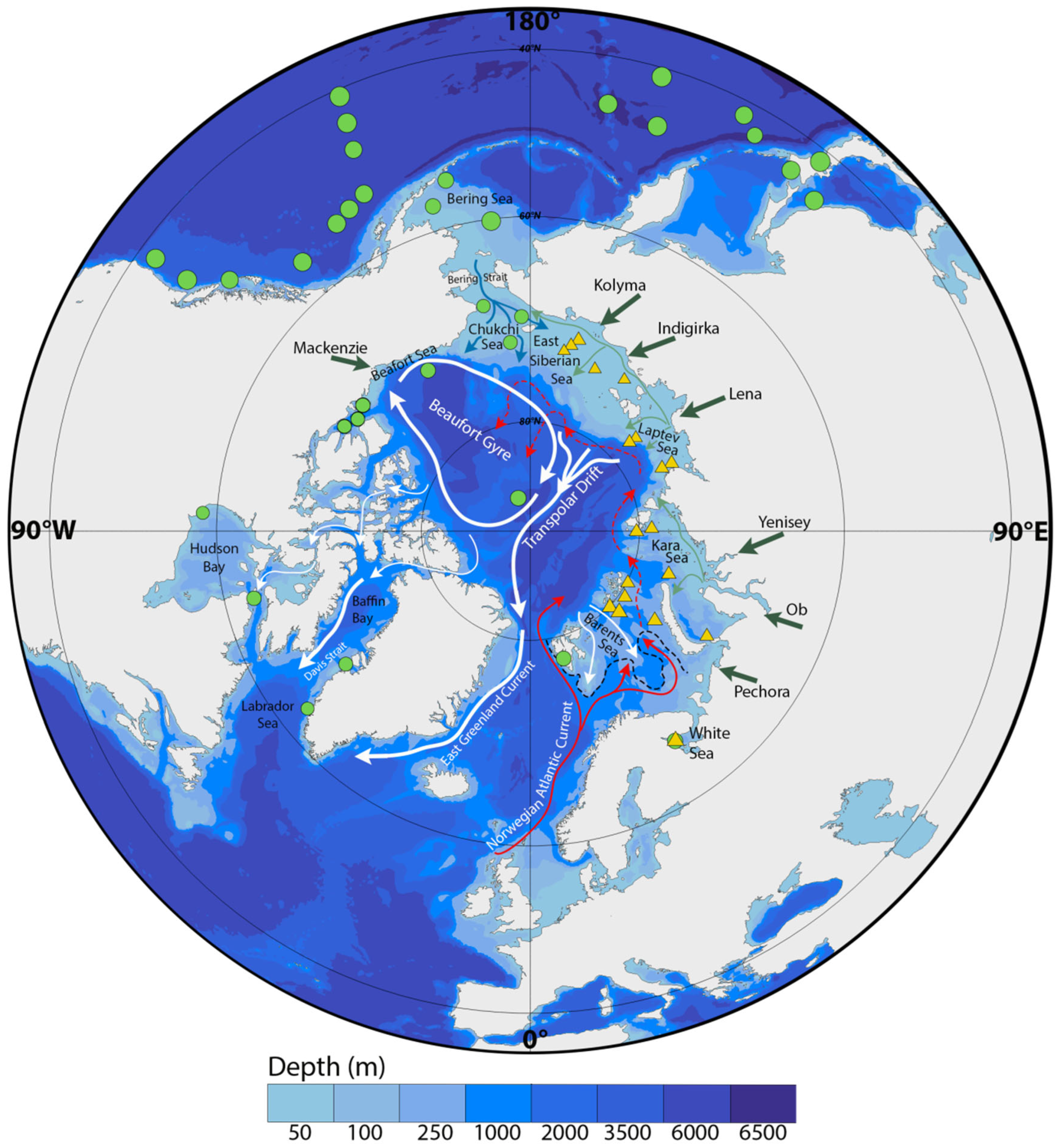
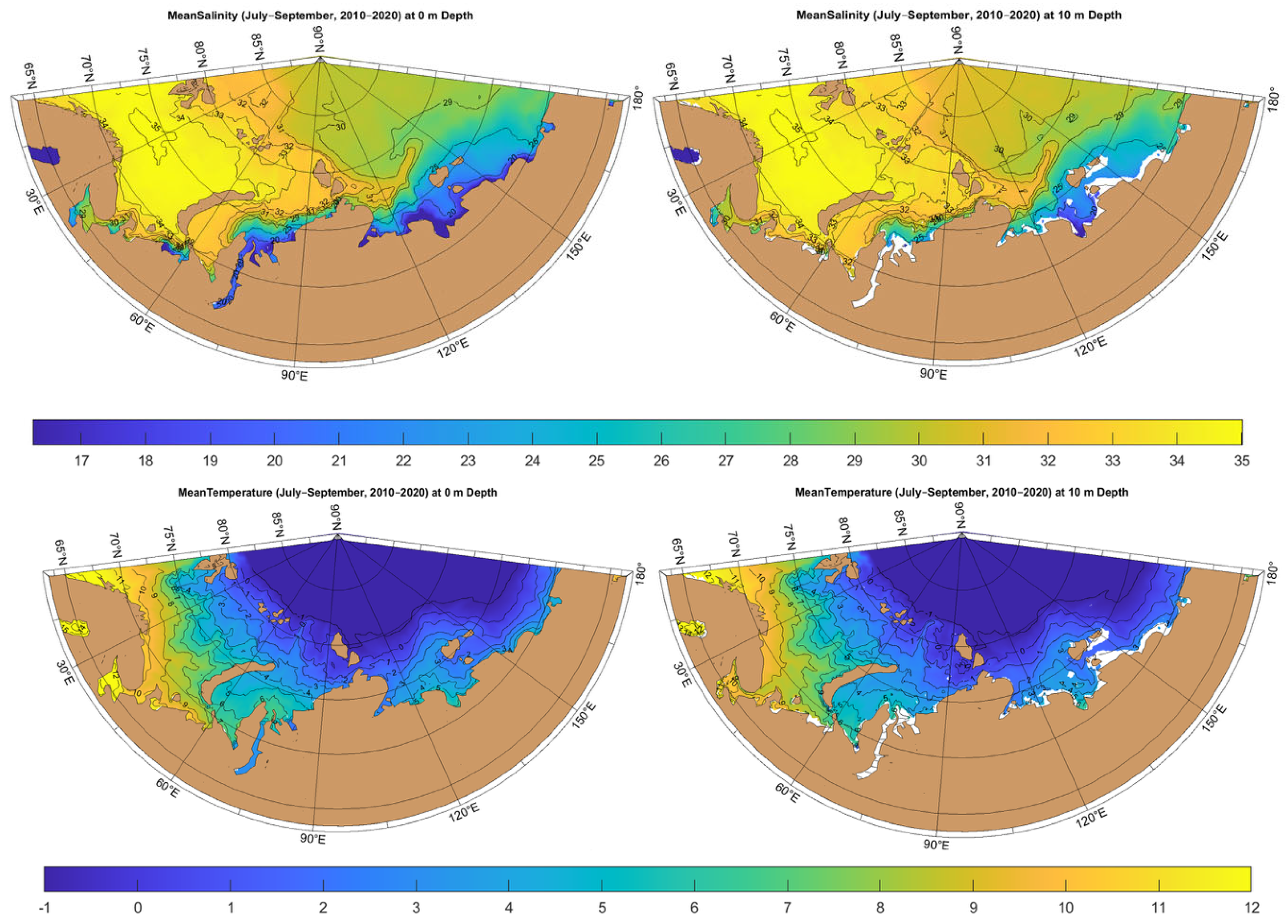
1.2. Regional Setting and Oceanographic Context of the Siberian Arctic Seas

The Eurasian Arctic shelf is a hydrographically complex region shaped by the convergence of Atlantic and Pacific water masses (Figure 1), large-scale freshwater input from major Siberian rivers, and seasonal sea ice dynamics. Surface and subsurface circulation is dominated by major current systems—including the Transpolar Drift, the Beaufort Gyre, and inflows via the Barents and Bering Straits—which structure the upper 200 m of the water column, the primary habitat of L. helicina [32,33,34,35,36,37]. These currents interact with freshwater plumes from the Ob, Yenisei, and Lena rivers [38,39], resulting in pronounced vertical stratification and horizontal salinity gradients that act as dispersal barriers and ecological filters. Climatological datasets (Figure 2) demonstrate sharp transitions between warm, saline Atlantic waters and cold, fresh Arctic regimes, influenced by river discharge and sea ice melt [40]. Together with bathymetric constraints, these hydrographic gradients establish semi-permeable ecological boundaries that regulate the dispersal and gene flow of pelagic organisms, contributing to the observed phylogeographic structuring of L. helicina and other Arctic zooplankton [41].

The Barents Sea, located at the Arctic–Atlantic transition zone, is characterized by the highest summer temperatures among the Arctic shelf seas, with surface waters warming up to 8–10 °C in the southern and southwestern regions (Figure 2), particularly near the Gorlo Strait connecting to the White Sea. This warming results from strong Atlantic water inflow (Figure 1), maintaining high thermal stability across much of the Barents Sea. South of the Polar Front, Atlantic-derived waters maintain salinities between 34.5 and 35.2 PSU and temperatures of 3–7 °C (Figure 2), whereas Arctic waters north of the front exhibit lower salinities (typically < 34.4 PSU) and temperatures approaching the freezing point, commonly between −1.5 and 1.5 °C [42]. The western fjords of Svalbard present an additional dynamic system, where the interplay of Atlantic and Arctic waters creates distinct hydrographic conditions that support a unique pelagic community structure [43]. This thermal and salinity front likely shapes biogeographic patterns of marine organisms and defines the southern range limit for cold-water species such as L. helicina, which are mostly confined to the colder, less saline waters north of the front [43,44].

The Kara Sea is significantly influenced by freshwater discharge from two of the largest Arctic rivers, the Ob and Yenisei (Figure 1), which together produce a low-salinity surface lens that dominates the hydrography during the ice-free season. In estuarine and coastal zones, surface salinity commonly drops to 10–20 PSU, with the freshened layer extending to depths of 20–30 m [45,46,47]. Beneath this lens, subsurface waters retain salinities of 33–34 PSU due to the intrusion of modified Atlantic waters (Figure 2). Surface temperatures vary spatially, exceeding 6–8 °C near river mouths but declining to around 0 °C offshore under Arctic water influence. At 10 m depth, salinity typically rises to ~30 PSU, though vertical stratification remains pronounced in nearshore areas. The hydrographic structure of the Kara Sea is thus defined by the interaction of three primary water masses: (1) warm, saline Atlantic-derived waters (salinity 34.5–35.2 PSU, temperature 3–7 °C), (2) colder Arctic-origin waters (salinity < 34.4 PSU, temperature between −1.5 and 1.5 °C), and (3) highly freshened riverine surface lenses (salinity 10–20 PSU, temperature > 6 °C near estuaries). The resulting horizontal and vertical gradients form persistent frontal zones that limit horizontal mixing and act as ecological boundaries [45,46]. Such hydrographic complexity generates spatially heterogeneous pelagic habitats and significantly shapes the distribution of marine communities. Cold-water pelagic species with limited tolerance to low salinity, such as L. helicina, are predominantly found in areas distant from major river mouths and estuaries—particularly along the southern and northwestern parts of the Kara Sea, near Novaya Zemlya and in the northern open shelf regions—where salinity and temperature conditions remain more stable [4,48,49].

The Laptev Sea is characterized by extreme seasonal variability, with extensive ice cover in winter and strong freshwater influence in summer, primarily from the Lena River [38,50]. The freshwater outflow creates a persistent surface lens with salinities ranging from 5 to 25 PSU, depending on seasonal discharge rates and mixing with underlying marine waters [51]. This freshened layer forms in the region of the Lena River plume and extends eastward via the East Siberian Current through the shallow Sannikov and Dmitry Laptev straits (Figure 1 and Figure 2), where it fills the entire water column due to limited depth, affecting the hydrography of adjacent shelf seas [51,52]. Summer surface temperatures in the Laptev Sea show clear spatial gradients, exceeding 6 °C near the Lena delta but dropping to approximately 0 °C towards the outer shelf and Arctic Basin (Figure 2). These thermal and salinity gradients play a crucial role in shaping estuarine frontal systems and restrict horizontal mixing during summer stratification [38,50]. Significantly, the shallow straits maintain extremely low salinities (17–23 PSU) during the summer season, limiting the distribution of marine species requiring higher salinities. As a result, cold-water species such as L. helicina, which prefer stable marine salinities, are largely absent from the heavily freshened nearshore zones of the Laptev Sea [53,54].

The East Siberian Sea is one of the least studied Arctic shelf seas but is known for its strong seasonal influence of riverine freshwater input and complex interactions with Pacific-derived water masses [50,55]. Unlike the Laptev and Kara Seas, where freshwater influence is largely constrained to the surface layers, river plumes in the East Siberian Sea can spread over broader areas due to wind-driven transport [39,50]. In addition, saline inflow from the Chukchi Sea, composed of Pacific-origin waters entering via the Bering Strait (Figure 1), contributes to the vertical and horizontal structuring of water masses in this region [34,56]. During summer, inner shelf areas are influenced by reduced salinity due to strong riverine input, with surface salinities dropping below 25 PSU (Figure 2). Salinity gradually increases toward the outer shelf, where conditions become more stable and marine-like. At greater depths, shelf waters remain more saline, often exceeding 32 PSU [38]. Surface temperatures during this period are relatively uniform across the region, typically ranging from –1 °C to 3 °C (Figure 2).

The Chukchi Sea acts as the primary gateway for Pacific waters entering the Arctic Ocean through the Bering Strait (Figure 1). The inflowing waters, which are relatively warm (–1 to 2 °C) and nutrient-rich compared to Arctic surface waters, are channeled into the Arctic Basin along three main branches: the Alaskan Coastal Current, the Central Channel, and the Herald Canyon flow [33]. These currents deliver Pacific-origin water masses to the Arctic halocline layer, influencing large-scale circulation via the Beaufort Gyre and Transpolar Drift [32,57]. The Pacific waters, typically exhibiting salinities of 31–33 PSU, can be traced across the Arctic Basin and into the Fram Strait, where they eventually mix with Atlantic-derived waters.

The White Sea stands out among the Arctic shelf seas as a semi-enclosed basin with distinct hydrographic characteristics. Its narrow connection to the Barents Sea through the Gorlo Strait restricts water exchange, while substantial riverine input and strong seasonal thermal stratification create a highly localized, estuarine-like environment. During summer, surface waters warm significantly, reaching up to 10–15 °C, while salinity often drops below 29 PSU due to freshwater inflow [58]. In winter, ice cover and surface cooling reestablish strong vertical mixing. These hydrographic features support a distinct planktonic community [59] and are expected to contribute the long-term genetic isolation of L. helicina populations within the White Sea. Unlike the more dynamic hydrographic settings of the Kara, Laptev, and East Siberian Seas, the White Sea’s semi-enclosed geography and distinct freshwater influence foster conditions that reinforce biological distinctiveness and restrict gene flow with surrounding Arctic populations.

2. Materials and Methods

2.1. Collection of Samples

Pteropods were collected using a Juday plankton net (vertical hauls, mouth area 0.1 m², mesh size 180 µm) from a depth of 0–170 m at 19 sampling locations (see Figure 1) across the Barents Sea, Kara Sea, Laptev Sea, and East Siberian Sea during August–September in various expeditions aboard the R/V Akademik Mstislav Keldysh between 2015 and 2019. Additionally, local samples were collected from the White Sea. Given the high mixing characteristics of pelagic environments and the absence of indications of vertical genetic structuring in pteropods, samples from the entire water column were pooled for genetic analyses. All expeditions and sample collections were conducted by scientists from the Shirshov Institute of Oceanology (Moscow, Russia) in collaboration with the Nikolai Pertsov White Sea Biological Station. Sampling coordinates are summarized in Supplementary File S1. Specimens were sorted on board, identified, and immediately preserved in 95% undenatured ethanol, then stored in freezers at −20 °C. All collected pteropods were subsequently transferred to the Shirshov Institute of Oceanology and the White Sea Biological Station for further study. The preserved samples form a foundational dataset for investigating the genetic diversity and population structure of Limacina helicina in the Arctic.

2.2. DNA Extraction, Amplification, and Sequencing

DNA was isolated from a piece of the pteropodia of large individuals (1–7 mm) or from the whole specimens in the case of small individuals (0.2–0.7 mm) using the ExtraGene^TM DNA Prep 100 kit (Isogen, Moscow, Russia) following the manufacturer’s protocol. A 625 bp fragment of the COI gene was amplified using Encyclo Plus PCR kit (Eurogen, Moscow, Russia) with the primers LCO-1490 (5′-GGTCAACAAATCATAAAGATATTGG-3′) and HCO-2198 (5′-TAAACTTCAGGGTGACCAAAAAATCA-3′) previously designed by Vrijenhoek et al., (1994) [60]. PCR was conducted under following conditions: initial denaturation at 95 °C for 5 min, followed by 39 cycles of 95 °C for 30 s, annealing at 50 °C for 45 s, and extension at 72° C for 1 min, with a final elongation at 72 °C for 8 min. Amplicons from successful PCR reactions were cleaned using either ExoSAP-IT™ Express PCR cleanup (ThermoFisher Scientific, Waltham, MA, USA) or the ethanol precipitation method. Sequencing was performed using an Applied Biosystems^® 3500 Genetic Analyzer by Eurogen and Syntol laboratories (Moscow, Russia).

A total of 189 specimens were successfully amplified (Supplementary File S1), including sequences from Barents, White, Kara, Laptev, and Eastern Siberian seas (all publicly available in GenBank).

2.3. Phylogenetic Analysis

Sequences were aligned using the MAFFT online tool Version 7.526 [61] which provides accurate and efficient multiple sequence alignment for DNA datasets. COI sequences were retrieved from consensus alignments of forward and reverse reads or, when necessary, from a single high-quality read. Resulting COI alignments were visually checked for errors and low quality contigs (contigs containing more than 3 Ns) were excluded from analysis. We additionally used all available data from the GenBank and BOLD databases (Supplementary File S1). The software Popart 1.7 [62] was then used for comparative analysis and the identification of differences between identified haplotypes through the construction of a TCS haplotype network [63]. The program DnaSP ver. 6 [64] was run for an estimation of haplotype diversity (hd) and nucleotide diversity (π), average number of nucleotide differences. The demographic history based on departures from neutrality, assuming random mating populations with no selection or recombination among DNA sequences, were assessed using Tajima’s D statistic [65] and Fu’s F test, both of which provide insights into past demographic events such as population expansions or contractions, as well as the potential influence of selection on genetic variation. Furthermore, the Arlequin 3.5 [66] software was used for pairwise φST calculations between regions analysis and verification of neutrality. Significance of φST was tested with 10,000 permutations. Additionally, the distribution of pairwise differences between haplotypes (mismatch distribution) was analyzed to estimate the parameters associated with the demographic population expansion. Sampling locations for this analysis were partitioned into geographic regions: Barents Sea, White Sea, Kara Sea, Laptev Sea, Eastern Siberian Sea, Northwest Pacific, Northeast Pacific, Bering Sea.

Divergence time estimations were performed using BEAST2 v2.7.7 [67]. As direct paleontological calibration points are not available for Limacina, we adopted a substitution rate of 0.0307 substitutions/site/Myr for gastropod COI, derived from closely related taxa with robust fossil records [68]. A maximum clade credibility tree with median node heights was generated in TREEANNOTATOR v2.7.7 and visualized using FigTree v1.4.4. The dated phylogeny was inferred under a strict molecular clock and a coalescent constant size tree prior. For Bayesian Skyline Plot analyses, we similarly employed BEAST2 with a strict clock at the same substitution rate (0.0307) and a coalescent Bayesian Skyline tree prior. Four major groups were analyzed independently (Arctic H1, Pacific H1, Arctic H2, White Sea H3) to reconstruct their demographic histories. Convergence for all BEAST2 runs was assessed using Tracer [69], confirming that all parameters achieved ESS values >1000; a 10% burn-in was applied for final analyses. The HKY model of nucleotide substitution was selected according to the Akaike Information Criterion implemented in IQ-TREE v1.6.12 [70] and subsequently applied in all BEAST2 analyses. A phylogenetic tree of haplotypes was also constructed in IQ-TREE using the same HKY model, with sequences of the closely related species Limacina retroversa serving as outgroup.

3. Results

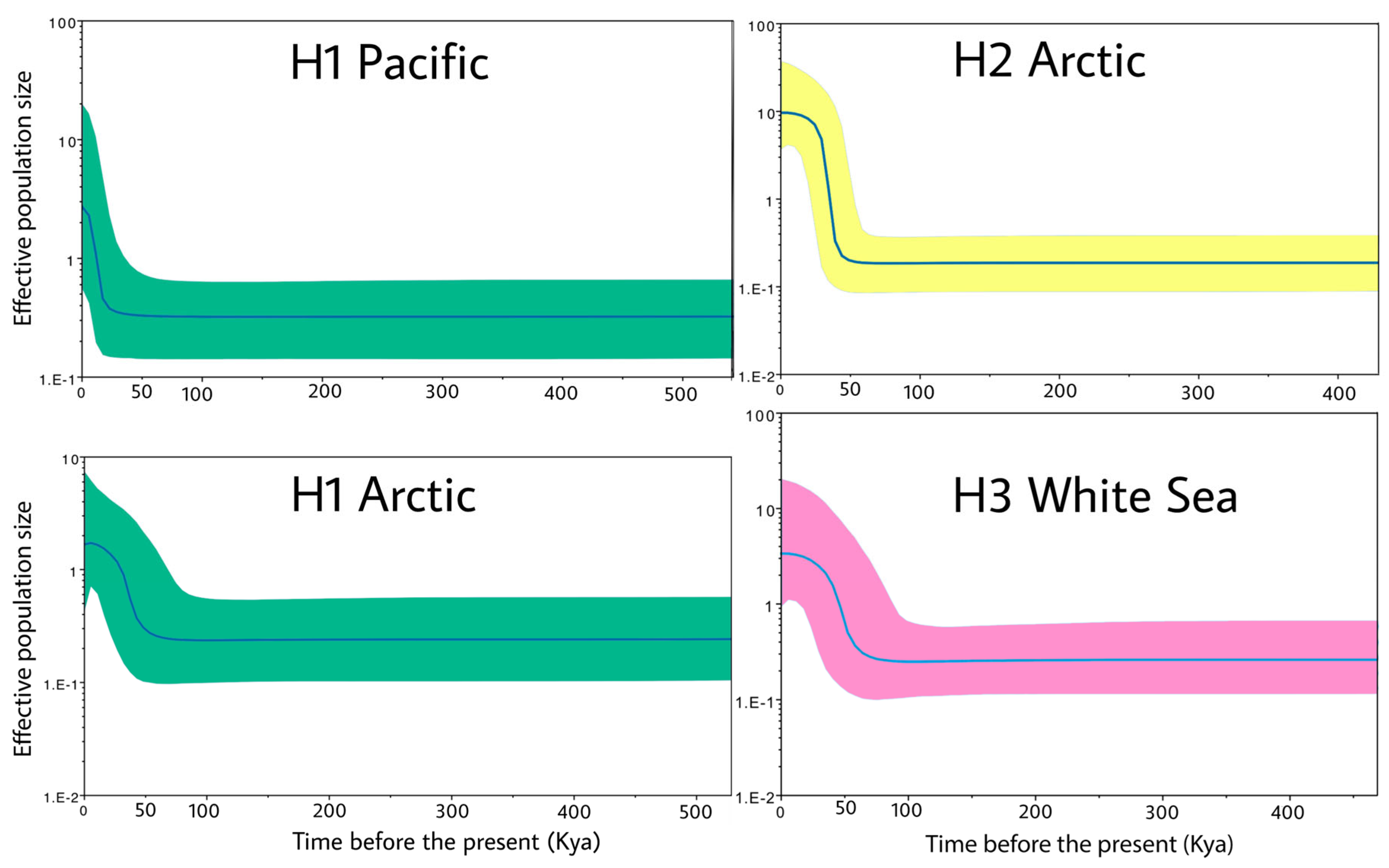
3.1. Population Structure and Demographic Patterns

A genetic analysis of the population of Limacina helicina, based on mitochondrial COI sequences from 873 individuals across Arctic seas, revealed substantial variability in haplotype (Hd) and nucleotide diversity (π), indicating notable differences in genetic diversity among regions (

Table 1. Population genetic statistics based on mitochondrial COI sequences for Limacina helicina across the Arctic region. Number of samples analyzed (N), sequence length in base pairs (bp), number of haplotypes (H), haplotype diversity (Hd) with standard deviation (SD), nucleotide diversity per site (π) with SD, Tajima’s D values with significance levels (p-values), and Fu’s Fs neutrality test results are indicated for each geographic population and for the total dataset.

Sample	N	BP	H	Hd	SD of Hd	π	SD of π	Tajima’s D	p-Value of Tajima’s D	Fu’s F
All data	873	503	161	0.61	0.019	0.00365	0.00045	−2.69815	<0.001	−358.121
White sea	48	555	18	0.66	0.08	0.00243	0.00055	−2.363	<0.01	−16.524
East Siberian	53	625	10	0.37	0.086	0.00102	0.00031	−2.31002	<0.01	−8.128
Laptev sea	41	556	23	0.86	0.051	0.0043	0.00064	−2.26034	<0.01	−20.508
Barents sea (Svalbard + Franz-Joseph land)	110	559	46	0.83	0.037	0.00426	0.00089	−2.6243	<0.001	−56.637
Svalbard (data of Sromek)	67	559	25	0.78	0.053	0.00313	0.00045	−2.2685	<0.01	−23.941
Franz-Joseph land	42	566	25	0.89	0.045	0.00383	0.00051	−2.16841	<0.01	−26.393
Kara sea	71	625	34	0.87	0.037	0.00369	0.00045	−2.39642	<0.01	−37.389
Bering sea	31	503	4	0.19	0.093	0.00038	0.0002	−1.73075	0.05 < p < 0.1 (not sign.)	−3.436
Pacific Alaska	116	503	12	0.23	0.052	0.00077	0.0002	−2.22414	<0.01	−13.859
Okhotsk sea	55	503	14	0.42	0.086	0.00101	0.00025	−2.49	<0.01	−18.404
NW Pacific	152	503	35	0.45	0.052	0.00161	0.00029	−2.72983	<0.001	−57.789
NE Pacific	157	503	5	0.08	0.029	0.00015	0.00006	−1.64582	0.05 < p < 0.1 (not sign.)	−7.212
Beaufort + Chukchi sea	19	503	3	0.21	0.119	0.00064	0.00041	−1.7188	0.05 < p < 0.1 (not sign.)	−1.085
Hudson + Greenland	15	503	8	0.88	0.06	0.0061	0.00091	−0.91604	0.05 < p < 0.1 (not sign.)	−1.624
Hudson	7	503	5	0.91	0.103	0.00682	0.001	0.26266	0.1 < p (not sign.)	−0.439
Greenland	8	503	5	0.86	0.108	0.00511	0.00121	−0.80566	0.1 < p (not sign.)	−0.61

). Overall, the dataset showed high haplotype diversity (Hd = 0.61) and relatively low nucleotide diversity (π = 0.00365).

Table 2. Pairwise Φ_ST distances between different geographic regions. Φ_ST values are below and p-values are above the diagonal. Significant values (p ≤ 0.05)—in bold, insignificant (p > 0.05)—regular font.

	Greenl.	Hudson	Beauf_Chuk	East_Sib	Fr_J_ land	Kara	Laptev	NE_ Pacific	NW_ Pacific	Okhot. Sea	Pacific_ Alaska	Pacific_ Bering	Svalb.	White Sea
Greenland		0.17117	0.000	0.000	0.000	0.000	0.03604	0.000	0.000	0.000	0.000	0.000	0.000	0.000
Hudson	0.05923		0.000	0.000	0.000	0.000	0.000	0.000	0.000	0.000	0.000	0.000	0.000	0.000
Beauf_Chuk	0.23189	0.32935		0.52252	0.000	0.000	0.000	0.03604	0.91892	0.80180	0.62162	0.67568	0.000	0.000
East_Sib	0.30044	0.43974	−0.00326		0.000	0.000	0.000	0.01802	0.12613	0.18919	0.05405	0.54955	0.000	0.000
Fr_J_land	0.18536	0.33321	0.52074	0.59073		0.16216	0.27928	0.000	0.000	0.000	0.000	0.000	0.46847	0.000
Kara	0.15107	0.31925	0.46101	0.51592	0.00631		0.69369	0.000	0.000	0.000	0.000	0.000	0.25225	0.000
Laptev	0.12261	0.26661	0.45171	0.52919	0.00281	−0.00502		0.000	0.000	0.000	0.000	0.000	0.42342	0.000
NE_Pacific	0.71162	0.80169	0.08923	0.02108	0.79234	0.69333	0.74534		0.000	0.000	0.000	0.04505	0.000	0.000
NW_Pacific	0.2671	0.41128	−0.01495	0.00359	0.61096	0.54526	0.5589	0.00856		0.26126	0.28829	0.83784	0.000	0.000
Okhot. Sea	0.31505	0.44495	−0.00636	0.00293	0.59231	0.51732	0.53047	0.01745	0.0023		0.04505	0.90991	0.000	0.000
Pacific_Alaska	0.39283	0.53688	−0.00676	0.01353	0.67048	0.58849	0.61627	0.02488	0.00033	0.01132		0.22523	0.000	0.000
Pacific_Bering	0.33733	0.44963	−0.00895	−0.00156	0.57062	0.49627	0.50389	0.03227	−0.00679	−0.00536	0.00468		0.000	0.000
Svalbard	0.20313	0.3732	0.52612	0.57473	−0.00258	0.00193	−0.00182	0.74716	0.59125	0.57651	0.64154	0.56053		0.000
White	0.43836	0.28695	0.45893	0.52389	0.59766	0.57111	0.5536	0.74588	0.52165	0.52546	0.59699	0.50967	0.61022

summarizes the genetic diversity indices calculated for each sampled region. Atlantic-influenced populations (Barents, Kara, and Laptev Seas) displayed high haplotype diversity (Hd = 0.83–0.89) and moderate to high nucleotide diversity (π = 0.00369–0.00426). These populations also showed significantly negative Tajima’s D and Fu’s Fs values, consistent with an excess of low-frequency polymorphisms. In contrast, Pacific populations (Bering Sea, NE and NW Pacific, Pacific Alaska) exhibited lower genetic diversity, particularly in haplotype richness (Hd = 0.08–0.45), with less pronounced signatures of population expansion. The East Siberian Sea population displayed the lowest overall diversity (Hd = 0.37; π = 0.00102), with negative but non-significant neutrality test results. The White Sea population exhibited intermediate haplotype diversity (Hd = 0.66), and relatively low nucleotide diversity (π = 0.00243) compared to most other regions. Neutrality tests yielded significantly negative Tajima’s D (−2.363, p < 0.01) and Fu’s Fs values (−16.524). This population was genetically distinct from all others, with consistently high ΦST values (e.g., >0.45), and a high number of private haplotypes. The matrix of pairwise nucleotide differences (Supplementary File S2) showed the highest divergence between Pacific populations and Franz Josef Land (>2.9 substitutions), while differences were lowest among geographically close Atlantic shelf seas (e.g., <1.5 substitutions between Kara, Laptev, and Barents Seas). These findings provide a baseline for understanding spatial genetic patterns in L. helicina and support the subsequent comparative analysis of genetic differentiation among Arctic and sub-Arctic populations.

Pairwise fixation indices (ΦST) (Table 2) further characterized regional genetic structure. Genetic differentiation was highest between Pacific and Atlantic populations, with ΦST values exceeding 0.5 in some pairwise comparisons (e.g., NE Pacific vs. Kara or Barents seas), and corresponding p-values indicating statistically significant divergence. In contrast, populations from adjacent Atlantic-influenced regions—such as the Barents, Kara, and Laptev seas—exhibited lower ΦST values (0.16–0.69) and lacked significant differentiation in many comparisons. The East Siberian Sea showed moderate differentiation from both Atlantic and Pacific regions. Despite its geographic proximity to the Laptev Sea, pairwise ΦST values between them were significant, suggesting limited gene flow across this boundary.

Samples from the Hudson Strait and the Greenland Sea were significantly differentiated from all other regions, with high ΦST values indicating restricted gene flow, trough no significant differences were found between the Hudson and Greenland populations themselves. The Barents, Kara, and Laptev Seas formed a cohesive group with low, non-significant ΦST values, dominated by haplogroup H2, while H1 was less common. The East Siberian Sea showed greater similarity to Pacific populations than to adjacent Atlantic regions, and pairwise comparisons indicated significant differentiation from the Laptev Sea. Both the East Siberian Sea and Pacific populations were exclusively composed of haplogroup H1, reinforcing the observed genetic affinity between these regions. Additionally, Svalbard and Franz Josef Land samples were not significantly different, supporting their grouping within the Barents Sea, and no internal structure was found across Kara Sea stations.

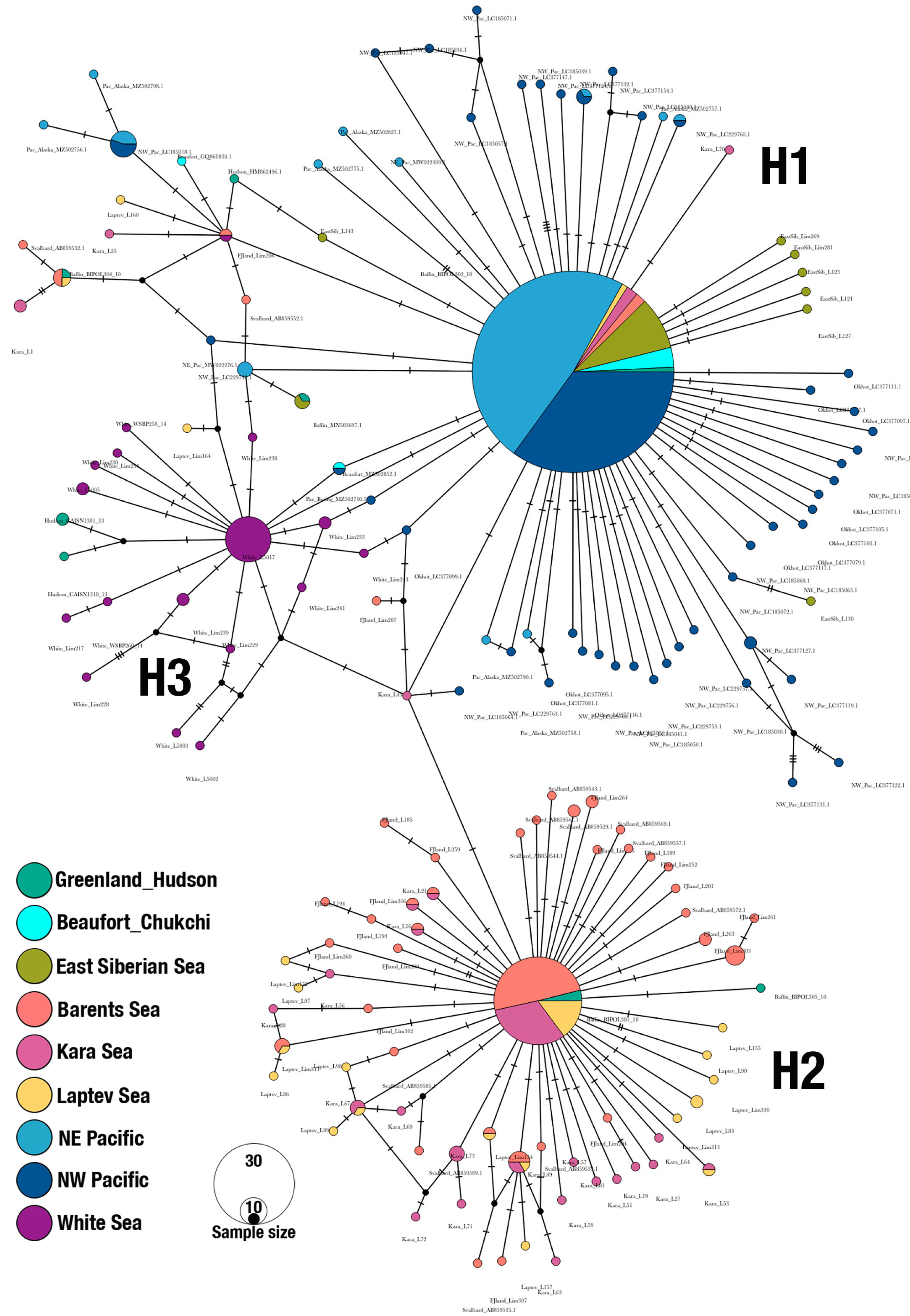
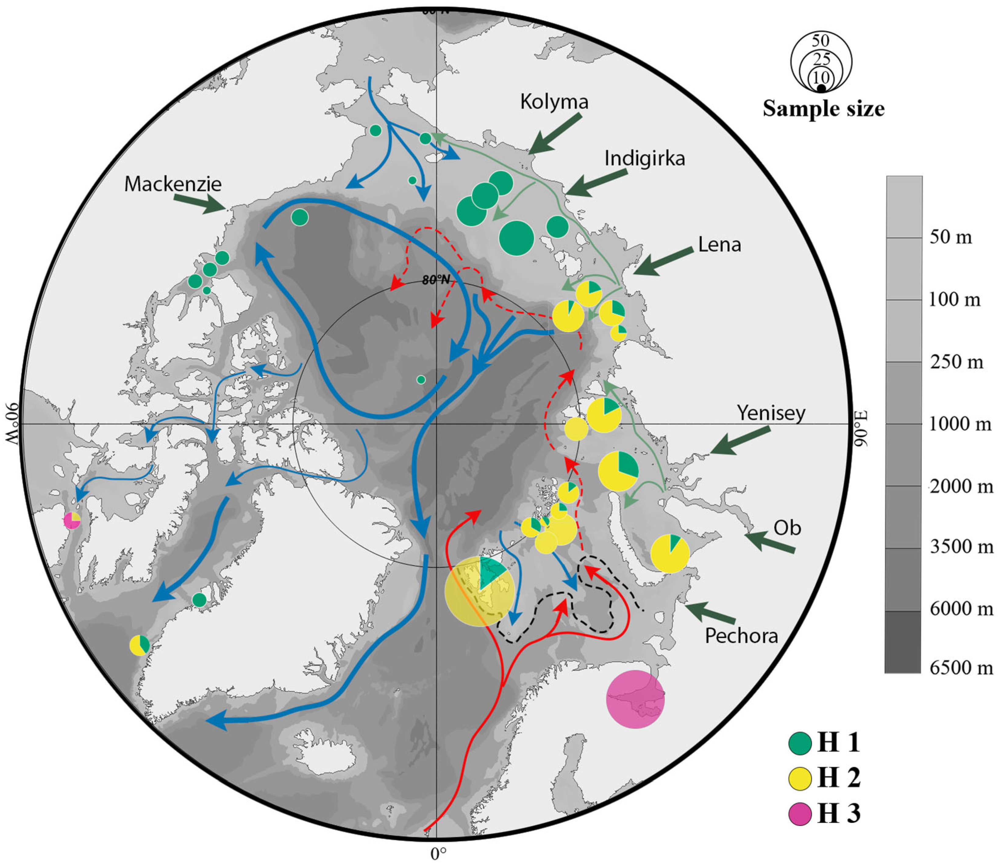
3.2. Haplogroups of Limacina helicina and Their Geographical Ranges

Three major haplogroups (H1, H2, H3) were identified within the mitochondrial COI dataset of L. helicina (Figure 3). These haplogroups exhibited distinct spatial distributions across the Arctic and sub-Arctic regions. Haplogroup H1 was the most widespread, dominating Pacific populations and also present in varying frequencies across other Arctic shelf regions (Figure 4). H2 occurred predominantly in the Barents, Kara, and Laptev Seas, where it frequently co-occurred with H1. Haplogroup H3 was found exclusively in the White Sea, where it was the only haplogroup detected and occurred at high frequency, characterized by a wide variety of private haplotypes indicating substantial local diversity.

The haplotype network (Figure 3) revealed clear genetic separation among the three haplogroups, with multiple mutational steps between them. H1 formed a large and highly connected cluster composed of several central and satellite haplotypes, predominantly from Pacific and East Siberian populations. H2 appeared as a distinct cluster with multiple internal branches, indicating greater haplotypic diversity within this group in the Barents–Kara–Laptev sector. H3 formed a compact and divergent clade, genetically distinct from H1 and H2, and composed almost entirely of unique haplotypes confined to the White Sea.

These patterns were further supported by our maximum likelihood haplotype tree that was reconstructed using IQ-TREE under the HKY model to illustrate relationships among haplotypes (Supplementary File S3), in which there were two well-supported monophyletic clades corresponding to H2 and H3, and a paraphyletic basal grade corresponding to H1. Despite the relatively shallow divergence observed in the haplotype network—typically only two to three mutational steps separating H1 and H2—the tree topology emphasizes the hierarchical separation of these lineages, underscoring their evolutionary distinctness and likely histories of past isolation. The outgroup sequences of L. retroversa clustered separately, confirming the clear genetic structuring observed within L. helicina.

The geographic distribution map (Figure 4) illustrates a distinct structuring of haplogroups across the Arctic. H1 dominated the Pacific regions, including NE Pacific, NW Pacific, Bering Sea, and Pacific Alaska, and extended into the East Siberian Sea. In contrast, H2 prevailed in the Atlantic-influenced Kara, Barents, and Laptev Seas. Some stations in these seas showed the co-occurrence of H1 and H2, though H2 remained dominant in most cases. H3 was found exclusively in the White Sea, with no evidence of its presence in neighboring basins.

We used time-calibrated phylogenetic trees constructed in BEAST2 to estimate the timing of divergence among major haplogroups of L. helicina (Supplementary File S4). Under a strict molecular clock with a rate of 0.0307 substitutions/site/Myr (derived from gastropod COI rates reported by Laakkonen et al., 2021) [68], we estimated that haplogroups H1 and H2 diverged approximately 320 kya (95% HPD: 200–450 kya), whereas the split between H1 and H3 occurred around 200 kya (95% HPD: 50–300 kya). However, applying a tenfold correction for elevated recent substitution rates, as suggested by Ho et al., (2011) [71] to account for time-dependent effects in shallow phylogenies, yielded considerably younger estimates of 32 Kya for H1–H2 divergence and 20 Kya for H1–H3, placing these events near the Last Glacial Maximum. Bayesian Skyline Plot analyses revealed evidence of substantial demographic expansions across all major haplogroups of L. helicina (Figure 5). Effective population size (Ne) was inferred to have increased by approximately 50-fold in haplogroup H2, and by around 10-fold in both H1 and H3 lineages. Based on the standard molecular clock rate, these expansions were dated to approximately 40–50 kya for Arctic H1, H2, and H3, and about 15–20 Kya for the Pacific H1 lineage. When recalibrated under the time-dependent rate correction, expansion times shifted to a much more recent period, occurring at approximately 4–5 kya for Arctic and White Sea populations, and around 2 kya for the Pacific population. Notably, the corrected timing for the H3 expansion closely aligns with the establishment of marine conditions in the White Sea following the last deglaciation, estimated at ~9 kya [72].

4. Discussion

4.1. Environmental Preferences and Habitat Conditions of Limacina helicina

Limacina helicina is known to have a narrow range of environmental preferences that define both its vertical and horizontal distribution: numerous studies have consistently demonstrated that this species is confined to cold water masses, with optimal temperatures ranging from approximately −1.6 °C to 4 °C, and an upper physiological threshold near 7 °C [5,6,36,37]. Temperatures above this range were shown to increase metabolic stress and mortality, particularly during overwintering phases [12,37]. Salinity is another critical environmental factor. Based on field data from Arctic shelf seas, L. helicina prefers waters with salinity levels above 30 PSU, with significantly higher biomass recorded in regions where salinity exceeds 33 PSU [48]. In contrast, in areas with salinity below 28 PSU—especially in regions influenced by freshwater discharge—L. helicina becomes rare or absent. This suggests that low salinity environments impose strong physiological constraints, including disrupted buoyancy and increased metabolic stress [5]. As a result, the combination of elevated temperature and reduced salinity acts as a powerful ecological barrier: regions where summer surface temperatures exceed 7 °C and salinity drops below 28 PSU are lacking this species.

Young L. helicina are mostly found in the top 50 m of the ocean, while adults can be found anywhere from the surface down to 200 m, all of them migrate diurnally within their depth ranges [35,36,73,74,75]. Seasonal shifts in vertical positioning have been documented: overwintering populations concentrate between 100 and 200 m depth, while in summer, they ascend toward surface layers to exploit seasonal peaks in primary production [37,75]. This adaptive migration strategy allows L. helicina to match its metabolic and reproductive cycles with regional productivity and environmental conditions.

In the seasonally melting ice-edge regions of the Arctic, L. helicina appears to exploit enhanced food availability associated with phytoplankton blooms triggered by the ice retreat [36,76]. Observations in the Barents Sea indicate that both juveniles and veliger larvae are concentrated in the surface waters during the periods of active melting, where stratified layers formed by freshwater input create favorable feeding conditions [77]. This seasonal aggregation suggests a behavioral adaptation to exploit short-lived peaks in primary production, particularly in late spring and summer, when phytoplankton is abundant near the surface. Previous research has also demonstrated that L. helicina can utilize organic material derived from melting sea ice and ice algae as a significant spring food source [36,75]. Although these surface layers are often characterized by reduced salinity, L. helicina may sustain such conditions when sufficient food is available. Nonetheless, prolonged exposure to salinity levels below 28 PSU can disrupt buoyancy control and increase energetic costs [5], making these conditions physiologically limiting. Consequently, summer regions with surface salinity persistently below 28 PSU and temperatures exceeding 7 °C likely represent exclusion zones for L. helicina, limiting both survival and reproductive success.

Regional data from the North Pacific show deviations from the typical Arctic distribution pattern. Limacina helicina has been recorded in surface layers where summer temperatures reach up to 8–9 °C, exceeding the conventional thermal tolerance range for this species [78]. Surface salinity in these regions generally ranges from 29 to 31 PSU, which, while slightly lower than Atlantic levels, remains typical for Pacific surface waters and appears suitable for L. helicina. In contrast to the Siberian Arctic shelf, where salinity can fall below 28 PSU due to massive riverine input, the North Pacific experiences less extensive freshwater influence [11,79]. As a result, no salinity-related exclusion zones have been reported in Pacific populations, and the weaker freshwater stratification may facilitate the persistence of this species across a broader temperature range. However, the localized upwelling zones and aragonite undersaturation in Pacific coastal areas, particularly along the continental shelf, may impose additional physiological stress on pteropods, especially at depth [12,80].

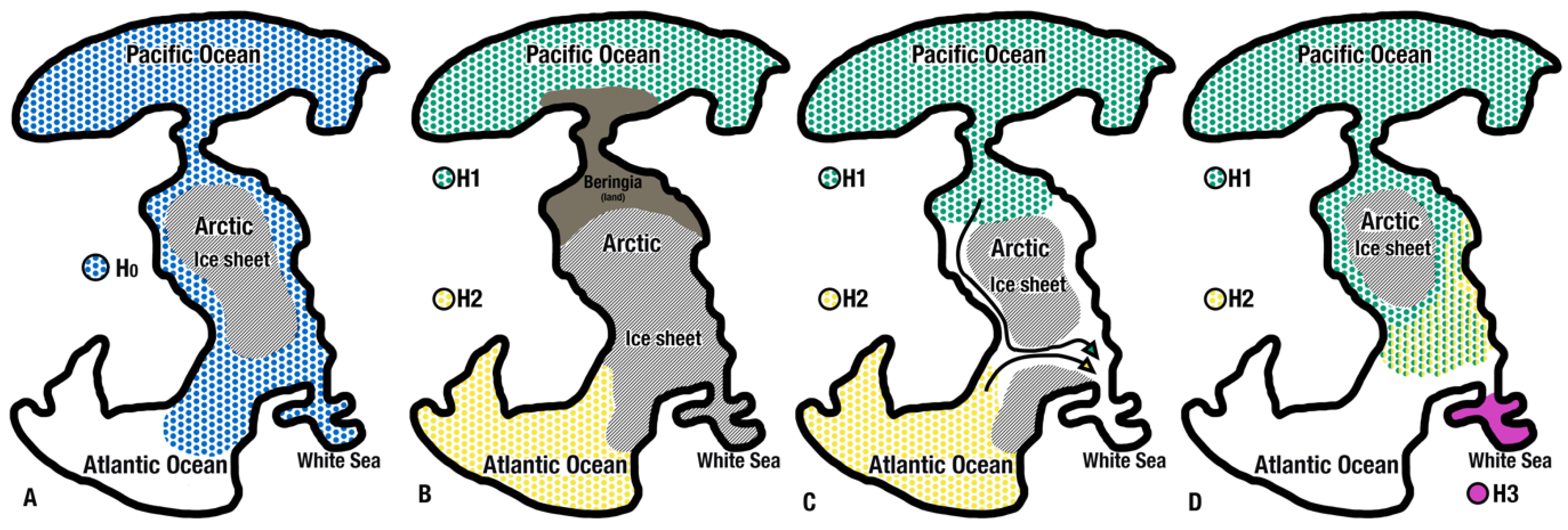
4.2. Palaeoecological Processes and Phylogeography

Pleistocene glaciations played a crucial role in shaping the contemporary genetic structure of L. helicina in the Arctic. During glacial maxima, extensive ice sheets covered the Arctic shelves (Figure 6), reducing available habitat and altering oceanic circulation [22,23]. This led to ecological fragmentation and isolation of planktonic populations, likely promoting divergence among distinct genetic lineages. During the Last Glacial Maximum (LGM, ~20 kya), the Barents, Kara, and Laptev Seas were largely covered by grounded ice or seasonal sea ice [81,82], restricting pelagic communities to southern regions or to localized, ice-free marine areas that offered suitable conditions for persistence [83,84,85]. The Bering Strait, now a major biogeographic gateway, began to shoal significantly around ~27 kya due to global sea-level fall, eventually closing completely by ~20 kya during the LGM with a drop of approximately ~120–130 m [22], halting Pacific–Arctic water exchange and effectively isolating populations of L. helicina in the Pacific and Atlantic basins. This isolation merely contributed to the divergence between haplogroups H1 (Pacific–Eastern Arctic) and H2 (Atlantic–Western Arctic). Our phylogenetic analyses provide direct genetic support for this paleogeographic scenario. Time-calibrated trees in BEAST2 indicate that haplogroups H1 and H2 diverged around 320 kya under a standard COI clock model (Supplementary File S4). However, applying time-dependent rate corrections [71], which account for generally accelerated substitution rates over recent evolutionary timescales, yields a more recent estimate of ~32 kya. This adjustment is especially relevant given the shallow divergence observed among haplogroups and is consistent with expectations for lineages affected by late Pleistocene climatic oscillations. Similarly, the divergence between H1 and the White Sea haplogroup H3 shifts from ~200 kya to ~20 kya under corrected rates, aligning closely with the LGM and maximum ice extent. These timelines suggest that while earlier Pleistocene glaciations may have initiated differentiation, the LGM was a critical period reinforcing genetic separation. This interpretation is further supported by our maximum likelihood phylogenetic tree of haplotypes (Supplementary File S3), which reveals two well-supported monophyletic clades corresponding to H2 and H3, alongside a paraphyletic basal assemblage representing H1. Although the haplotype network shows only two to three mutational steps between H1 and H2, the tree topology underscores their hierarchical separation, pointing to historical isolation followed by subsequent demographic expansion. The distinct positioning of H3 as an exclusive lineage confined to the White Sea underscores its unique evolutionary trajectory relative to the broader Arctic and Pacific populations.

The postglacial reopening of the Bering Strait around 11–12 ka [86] re-established Pacific inflows, facilitating the recolonization of Arctic regions by Pacific species [87], including L. helicina. As the ice margin continued its northward retreat throughout the Holocene, newly exposed shelf habitats across the Arctic became available for colonization [79,86], supporting the expansion of both major haplogroups. Bayesian Skyline analyses further indicate that all lineages underwent substantial demographic growth following these climatic shifts, with effective population sizes increasing approximately ~50-fold for H2 and ~10-fold for H1 and H3. While standard molecular clocks place these expansions around ~40–50 kya, applying time-dependent rate corrections shifts them to ~4–5 kya, aligning closely with the late Holocene marine transgression and the final deglaciation of Arctic shelf seas. This temporal correspondence underscores how deglacial processes created extensive new habitats that drove rapid postglacial expansions, particularly of the Pacific-derived haplogroup H1 as it advanced through the reopened Bering gateway into the Arctic basin.

Although isolated ice-free polynyas have been suggested as potential refugia within the Arctic itself [22,88], it is more likely that L. helicina populations persisted primarily in stable ice-free areas of the Norwegian Sea and northwestern Atlantic in the Labrador Sea, characterized by relatively consistent thermal and salinity conditions. These regions maintained relatively consistent thermal and salinity regimes even during peak glacial conditions and are considered to have served as important northern Atlantic refugia for cold-adapted marine species [84,89]. The presence of such stable conditions in the Norwegian Greenland sector would have supported small, viable planktonic populations and subsequently facilitated the recolonization of Arctic shelf seas as the ice retreated (Figure 6C). As deglaciation progressed throughout the Holocene, the gradual northward shift in the ice edge created new ecological space for expansion, while the retreating margin itself acted as a dynamic biogeographic filter structuring species distributions [86]. The contemporary distribution of L. helicina haplogroups H1 and H2 is consistent with this scenario of postglacial expansion from separate refugial sources, followed by secondary contact in central Arctic shelf areas. Haplogroup H1, dominant in the Pacific sector and Eastern Arctic, likely entered through the reopened Bering Strait and spread westward via the Transpolar Drift. In contrast, haplogroup H2, likely originating from ice-free Atlantic refugia, expanded eastward across the Barents, Kara, and Laptev Seas, reflecting the west-to-east trajectory of deglaciation along the Eurasian shelf [22,23].

Postglacial recolonization scenarios identified for L. helicina are supported by research on other Arctic zooplankton species. For example, Calanus glacialis expanded its range following the LGM from presumed Pacific refugia into the Arctic and subsequently into the Atlantic [90], accompanied by rapid population growth and increased productivity in Arctic seas during the early Holocene (~10 thousand years ago) [27,89]. Similar processes have been described for Pseudocalanus spp., whose Arctic species show strong population connectivity supported by both historical migrations and contemporary hydrographic links between basins [24,26,91]. A distinct genetic structure has also been detected in the euphausiid Thysanoessa inermis [28], with a clear separation between North Pacific and Eurasian Arctic populations, mirroring the patterns found in L. helicina and underscoring the similarity of phylogeographic scenarios across Arctic pelagic communities.

Haplogroups H1 and H2 form star-like haplotype network topologies with only two mutational steps separating them, suggesting recent divergence events associated with postglacial expansion [16,20,21]. These patterns are further corroborated by neutrality tests (negative Tajima’s D and Fu’s Fs), indicating excesses of rare alleles typical for populations that experienced historical bottlenecks followed by rapid growth [20,27], as well as by our Bayesian Skyline Plot analyses showing sharp increases in effective population size for these haplogroups (Figure 5). Low nucleotide diversity paired with high haplotype richness in L. helicina further supports a demographic scenario involving severe population reductions during glacial maxima and rapid expansions during interglacial periods [20,27]. Thus, the observed genetic patterns of L. helicina—with distinct eastern (H1) and western (H2) Arctic haplogroups and a third unique group in the White Sea—mirror the influence of glacial history, asynchronous postglacial recolonization, and differential dispersal routes from both Pacific and Atlantic source regions [85,89,92].

4.3. Contemporary Hydrographic Barriers and Their Influence on the Distribution of L. helicina

The present-day oceanographic structure of the Arctic significantly shapes the population connectivity and genetic structure of L. helicina. Three distinct haplogroups (H1, H2, H3) display marked geographic partitioning that aligns with known hydrographic features (Figure 4). Major hydrographic features such as large-scale ocean currents, polar fronts, and freshwater discharges from major Arctic rivers define a complex mosaic of water masses and stratification patterns that structure planktonic biodiversity. Haplogroup H1 is the most widely distributed, dominating in the Pacific sector [8,9,21,93] and extending throughout the Eastern Arctic—including the Chukchi, Beaufort, and East Siberian Seas—and further westward across the Arctic Basin via the Transpolar Drift (Figure 4), reaching as far as Greenland and the Fram Strait. This broad distribution reflects the influence of postglacial recolonization and sustained connectivity through Pacific inflow via the Bering Strait, which reopened at ~11–12 ka [90], and east-to-west advection through the Transpolar Drift. The predominance of haplogroup H1 in both Pacific and central Arctic regions suggests a high dispersal capacity and broad environmental tolerance, enabling persistence across diverse Arctic shelf conditions. Haplogroup H2 is restricted to the Western Arctic and occurs only in the Barents, Kara, and Laptev Seas. Its absence in the East Siberian Sea suggests the presence of strong ecological barriers to eastward dispersal. One such barrier is the intense freshwater discharge from the Lena River, which forms a low-salinity surface plume that can dominate the upper water column during summer [38]. This freshened layer often extends into the Sannikov and Dmitry Laptev Straits, which are relatively shallow and thus dominated by riverine outflow in the ice-free season. Under such conditions L. helicina becomes rare or absent. Observations from the southern Laptev, East Siberian, and central Kara Seas near estuarine zones confirm the absence of L. helicina in highly diluted waters, forming a recognizable “limacine-free zone” [4,94]. Field studies show the biomass fall when salinity decreases to 30 PSU or less, and individuals are not found in waters below 28 PSU. Although subsurface Atlantic-derived waters occasionally reach the East Siberian Sea along the continental slope, these currents occur below 300 m [95], while L. helicina is mostly confined to the upper 200 m of the water column, limiting its access to these intruding saline waters. This supports the hypothesis that H2 persists and recirculates primarily within the western Arctic shelves, i.e., namely the Barents, Kara, and Laptev Seas, through the Transpolar Drift, without eastward expansion beyond freshwater-dominated barriers. Even if occasional advection of individuals occurs, the absence of H2 in the East Siberian Sea suggests potential post-settlement exclusion due to unfavorable conditions or competitive genetic displacement.

The Barents Sea additionally illustrates the role of hydrographic fronts in delimiting pteropod distributions. The Polar Front, which separates colder Arctic waters from the warmer Atlantic inflow, functions as a pronounced ecological boundary. Observations from previous studies and our own data indicate that L. helicina is largely restricted to waters north of this front, where summer temperatures typically remain below 6 °C and salinity exceeds 33 PSU [44,76,96]. Genetic analysis shows that the populations of L. helicina in the Barents Sea contain both H1 and H2 haplogroups, with H2 being dominant, reflecting the Atlantic–Arctic nature of the basin and its strong hydrographic connectivity with neighboring seas. In contrast, L. retroversa, a more thermophilic congener, dominates the southern Barents Sea under the influence of Atlantic waters. Although the two species may occasionally co-occur near the front, they remain reproductively isolated, and L. helicina does not establish persistent populations south of the front.

The White Sea haplogroup H3 represents a remarkable case of localized genetic isolation in a semi-enclosed basin. Although there is seasonal inflow of saline Atlantic water through the Gorlo Strait, the White Sea maintains a stratified hydrographic regime with a strong surface freshening due to river input and ice melt [58]. Genetic data indicate no haplotype exchange with adjacent Arctic populations. This isolation is further reinforced by the absence of L. helicina in the southern Barents Sea under strong Atlantic influence, where summer surface temperatures commonly exceed 8–10°, crossing the species’ upper thermal limit. This pattern is supported by both our data and other studies [44,96] thus suggesting that the southern stations influenced by Atlantic water are consistently devoid of L. helicina. As a result, the White Sea population remains isolated by warm waters to the north and by local hydrographic conditions, including lower salinity and strong seasonal stratification.

Contemporary Arctic circulation systems, including the Transpolar Drift, Beaufort Gyre, and Atlantic inflow via the Barents Sea, continue to redistribute zooplankton across the basin [32]. However, despite the potential for widespread dispersal, L. helicina populations show discrete haplogroup boundaries that align with prominent hydrographic features, such as freshwater fronts, narrow straits, and salinity gradients. These patterns reflect the interaction of historical isolation, contemporary circulation, and the species’ physiological sensitivity to environmental parameters such as temperature and salinity, as well as ecological constraints related to food availability and vulnerability to ocean acidification [4,8,75,80].

4.4. The White Sea: Isolation and Local Population Specificity

The L. helicina population in the White Sea (H3) represents a unique case of spatial isolation, likely driven by adaptation to local hydrographic conditions that differ significantly from those of other Arctic regions. Isolating factors for the White Sea population of L. helicina include reduced salinity and strong seasonal temperature dynamics, both of which limit the penetration of planktonic organisms from the Barents Sea. Given the species’ known sensitivity to low salinity [4], the persistence of L. helicina in the White Sea likely required specific adaptations to survive under these unique local conditions. These environmental characteristics may have facilitated the establishment of a distinct haplogroup (H3), maintained by the stability of hydrographic barriers. The genetic structure of the White Sea L. helicina population further substantiates its relative isolation. The haplotype network of this group exhibits a distinct star-like pattern, accompanied by low nucleotide diversity—both of which are characteristic of a recent demographic expansion following a population bottleneck [84,97]. This interpretation is supported by significantly negative values from neutrality tests such as Tajima’s D and Fu’s Fs. Importantly, haplotypes specific to the White Sea are absent in other surveyed Arctic regions, reinforcing the notion of restricted gene flow and localized persistence of this population.

Our divergence time estimated from BEAST analyses adds further context to these patterns, indicating that the divergence between H1 and the White Sea haplogroup H3 shifts from approximately ~200 kya under a standard molecular clock to around ~20 kya when applying time-dependent rate corrections [71]. This timing aligns closely with the Last Glacial Maximum and suggests that while earlier Pleistocene glaciations may have initiated lineage differentiation, the LGM likely played a critical role in reinforcing genetic separation and facilitating the emergence of H3 as a distinct lineage. Therefore, the formation of the White Sea population most likely occurred during the postglacial period (Figure 6C), when Atlantic water exchange resumed, allowing the species to recolonize the basin. The initial colonization could have involved individuals from both the Pacific-derived H1 and Atlantic-derived H2 haplogroups, which dispersed into the Arctic Ocean following the retreat of glacial ice. However, despite this possibility, our phylogenetic analyses (Supplementary File S3) indicate that H3 shares closer affinities with the Pacific H1 lineage than with H2, as reflected by their positions in the tree topology. This suggests that the White Sea population may have been primarily seeded by H1-like lineages, which represent a Pacific group that recolonized the Arctic only after the retreat of the ice sheets, during early postglacial periods. Alternatively, it is also possible that H3 represents a remnant of a more broadly distributed lineage that persisted in marine refugia such as the Labrador Sea, which remained partially ice-free during certain intervals of the last glacial maximum. This interpretation finds tentative support in the presence of three individuals from the Hudson Strait that carry haplotypes which are the most similar to those found in the White Sea (CAISN1301, CAISN1302, CAISN1310). Further studies expanding sampling efforts in these regions could help clarify the broader historical distribution of this lineage. Subsequent prolonged local isolation under unique hydrographic conditions within the White Sea likely facilitated independent demographic expansion, ultimately giving rise to the distinct genetic structure observed today.

Historically, it is unlikely that the White Sea served as a refugium for L. helicina during the Last Glacial Maximum (LGM), when much of the basin experienced significant freshening and partial isolation. Unlike species such as smelt (Osmerus dentex) and herring (Clupea pallasii), which are capable of surviving in both fresh and brackish waters [98,99], L. helicina remains a strictly marine species that requires high-salinity conditions. Subsequent isolation due to local hydrographic conditions—such as strong seasonal stratification and limited water exchange through the Gorlo Strait—likely promoted the independent emergence and long-term persistence of the distinct H3 haplogroup in the White Sea. In addition to smelt and herring, similar localized populations in the White Sea have been reported in benthic taxa such as the nudibranch Onchidoris muricata [100], which reveal contemporary microevolutionary processes in this basin. An additional support for the existence of the L. helicina population in the White Sea may be linked to ice edges and areas of elevated primary productivity [76]. It is possible that, historically, the White Sea population tracked ice edges, as observed in other Arctic planktonic species such as Calanus glacialis, which are adapted to the high productivity of ice-edge zones [95,101]. Contemporary seasonal dynamics in the White Sea, including winter ice cover and summer warming, maintain such conditions, creating a favorable environment for population stability.

5. Conclusions: Implications for Arctic Pelagic Dynamics and Future Projections

Our data allow both reconstruction the species’ colonization history in the Arctic and assessment of the key ecological and climatic factors that continue to population structure of this pelagic mollusk. The high sensitivity of L. helicina to hydrographic gradients, as well as to historical shifts in water mass circulation, makes this species a valuable indicator of ongoing processes in the Arctic pelagic ecosystem.

The identified phylogeographic structuring in L. helicina, characterized by three geographically distinct haplogroups across the Arctic, illustrates the complex interplay of historical isolation, subsequent dispersal events, and contemporary oceanographic influences. The combination of high haplotype and low nucleotide diversity found across the three haplogroups of L. helicina aligns with common demographic patterns in marine planktonic organisms influenced by climatic oscillations during the Pleistocene [20]. Similar demographic histories have been documented in critical Arctic zooplankton species, including Calanus glacialis, Pseudocalanus spp., Thysanoessa inermis, and Eukrohnia hamata [24,25,27,28,91]. These studies highlight the significant role of historical climate-driven expansions from glacial refugia, resulting in current widespread distribution yet relatively low genetic diversity within these taxa.

In the context of modern Arctic transformation—characterized by warming, reduction in sea ice extent, alterations in water mass transport, and increased freshwater input—L. helicina populations are a subject to multiple simultaneous pressures. Previous studies [13,78] have shown that this species is particularly vulnerable to ocean acidification due to the mineral composition of its aragonite shell. The ongoing decline in pH and the increased solubility of aragonite in Arctic surface waters are already causing elevated levels of shell dissolution in L. helicina, posing a significant risk of population declines in the near future. Additionally, changes in water mass exchange between oceanic basins associated with increased Atlantic water inflow into the Eastern Arctic and shifts in the strength of the Transpolar Drift may alter the current boundaries between phylogeographic groups. In particular, the ongoing Atlantification of the Barents and Kara Seas could lead to a shift in the range of haplogroup H2, associated with the Atlantic sector of the Arctic, and its expansion into eastern regions. Similar range shifts have been observed in other key zooplankton species, such as Calanus glacialis, which has been moving northward in response to the retreating sea ice edge [27,87]. These observations demonstrate that the phylogeographic structure of Arctic organisms is dynamic and responsive to changes in the climate system. It can be assumed that with further warming and decreasing salinity in surface waters driven by intensified river discharge and ice melt, the suitable habitats for L. helicina will shrink, particularly for populations preferring higher salinity conditions, such as H1 and H2. This could lead to local extinctions or significant population declines, especially in the Eastern Arctic, where freshwater influence is most pronounced. Meanwhile, the White Sea population (H3), which has adapted to lower salinity conditions, may remain stable under these changes but will likely continue to be restricted to its localized environment. The White Sea haplogroup thus represents a striking example of how unique hydrographic and climatic conditions can foster long-term isolation and independent evolution of marine plankton populations. Its emergence likely reflects a combination of postglacial colonization by H1-like lineages, subsequent demographic expansion under the constraints of reduced salinity and pronounced seasonal stratification, and continued separation maintained by hydrographic barriers—most notably the inflow of warmer Atlantic waters into the southern Barents Sea, which limits the southward extent of colder Arctic water masses toward the White Sea. Looking ahead, the ongoing warming of Barents Sea waters and alterations in Arctic circulation are expected to further enhance the isolation of the White Sea from the broader Arctic faunal exchange, potentially reinforcing the distinct evolutionary trajectory of its endemic planktonic lineages.

Overall, our findings offer an essential baseline for monitoring changes in Arctic biodiversity amid ongoing climate transformations. Continuous tracking of haplogroup distributions and haplotype compositions can provide insights into the dynamics and extent of Arctic ecosystem reorganization. This approach will also aid in identifying regions demonstrating ecological resilience or those increasingly vulnerable to environmental degradation, a task of growing urgency given the accelerating pace of Arctic climate change.

References

1. Lalli, C.M.; Gilmer, R.W. The Thecosomes, Shelled Pteropods. In Pelagic Snails. The Biology of Holoplanktonic Gastropod Mollusks; Lalli, C.M., Gilmer, R.W., Eds.; Stanford University Press: Stanford, CA, USA, 1989; pp. 58–166. [Google Scholar]
2. Hunt, B.P.V.; Pakhomov, E.A.; Hosie, G.W.; Siegel, V.; Ward, P.; Bernard, K. Pteropods in Southern Ocean Ecosystems. Prog. Oceanogr. 2008, 78, 193–221. [Google Scholar] [CrossRef]
3. Doubleday, A.J.; Hopcroft, R.R. Interannual Patterns during Spring and Late Summer of Larvaceans and Pteropods in the Coastal Gulf of Alaska, and Their Relationship to Pink Salmon Survival. J. Plankton Res. 2015, 37, 134–150. [Google Scholar] [CrossRef]
4. Pasternak, A.F.; Drits, A.V.; Gopko, M.V.; Flint, M.V. Influence of Environmental Factors on the Distribution of Pteropods Limacina Helicina (Phipps, 1774) in Siberian Arctic Seas. Oceanology 2020, 60, 490–500. [Google Scholar] [CrossRef]
5. Gilmer, R.; Harbison, G. Diet of Limacina Helicina (Gastropoda: Thecosomata) in Arctic Waters in Midsummer. Mar. Ecol. Prog. Ser. 1991, 77, 125–134. [Google Scholar] [CrossRef]
6. Bé, A.W.H.; Gilmer, R.W. A Zoogeographic and Taxonomic Review of Euthecosomatous Pteropoda. In Oceanic Micropaleontology; Academic Press: Cambridge, MA, USA, 1977; pp. 733–808. [Google Scholar]
7. Guinotte, J.M.; Fabry, V.J. Ocean Acidification and Its Potential Effects on Marine Ecosystems. Ann. N. Y. Acad. Sci. 2008, 1134, 320–342. [Google Scholar] [CrossRef]
8. Bednaršek, N.; Naish, K.-A.; Feely, R.A.; Hauri, C.; Kimoto, K.; Hermann, A.J.; Michel, C.; Niemi, A.; Pilcher, D. Integrated Assessment of Ocean Acidification Risks to Pteropods in the Northern High Latitudes: Regional Comparison of Exposure, Sensitivity and Adaptive Capacity. Front. Mar. Sci. 2021, 8, 671497. [Google Scholar] [CrossRef]
9. Mekkes, L.; Renema, W.; Bednaršek, N.; Alin, S.R.; Feely, R.A.; Huisman, J.; Roessingh, P.; Peijnenburg, K.T.C.A. Pteropods Make Thinner Shells in the Upwelling Region of the California Current Ecosystem. Sci. Rep. 2021, 11, 1731. [Google Scholar] [CrossRef]
10. Orr, J.C.; Fabry, V.J.; Aumont, O.; Bopp, L.; Doney, S.C.; Feely, R.A.; Gnanadesikan, A.; Gruber, N.; Ishida, A.; Joos, F.; et al. Anthropogenic Ocean Acidification over the Twenty-First Century and Its Impact on Calcifying Organisms. Nature 2005, 437, 681–686. [Google Scholar] [CrossRef]
11. Niemi, A.; Bednaršek, N.; Michel, C.; Feely, R.A.; Williams, W.; Azetsu-Scott, K.; Walkusz, W.; Reist, J.D. Biological Impact of Ocean Acidification in the Canadian Arctic: Widespread Severe Pteropod Shell Dissolution in Amundsen Gulf. Front. Mar. Sci. 2021, 8, 600184. [Google Scholar] [CrossRef]
12. Comeau, S.; Jeffree, R.; Teyssié, J.-L.; Gattuso, J.-P. Response of the Arctic Pteropod Limacina Helicina to Projected Future Environmental Conditions. PLoS ONE 2010, 5, e11362. [Google Scholar] [CrossRef]
13. Manno, C.; Bednaršek, N.; Tarling, G.A.; Peck, V.L.; Comeau, S.; Adhikari, D.; Bakker, D.C.E.; Bauerfeind, E.; Bergan, A.J.; Berning, M.I.; et al. Shelled Pteropods in Peril: Assessing Vulnerability in a High CO2 Ocean. Earth-Sci. Rev. 2017, 169, 132–145. [Google Scholar] [CrossRef]
14. Buitenhuis, E.T.; Le Quéré, C.; Bednaršek, N.; Schiebel, R. Large Contribution of Pteropods to Shallow CaCO3 Export. Glob. Biogeochem. Cycles 2019, 33, 458–468. [Google Scholar] [CrossRef]
15. Burridge, A.K.; Hörnlein, C.; Janssen, A.W.; Hughes, M.; Bush, S.L.; Marlétaz, F.; Gasca, R.; Pierrot-Bults, A.C.; Michel, E.; Todd, J.A.; et al. Time-Calibrated Molecular Phylogeny of Pteropods. PLoS ONE 2017, 12, e0177325. [Google Scholar] [CrossRef]
16. Abyzova, G.A.; Nikitin, M.A.; Popova, O.V.; Pasternak, A.F. Genetic Population Structure of the Pelagic Mollusk Limacina Helicina in the Kara Sea. PeerJ 2018, 6, e5709. [Google Scholar] [CrossRef]
17. Janssen, A.W.; Bush, S.L.; Bednaršek, N. The Shelled Pteropods of the Northeast Pacific Ocean (Mollusca: Heterobranchia, Pteropoda). Zoosymposia 2019, 13, 305–346. [Google Scholar] [CrossRef]
18. Choo, L.Q.; Bal, T.M.P.; Choquet, M.; Smolina, I.; Ramos-Silva, P.; Marlétaz, F.; Kopp, M.; Hoarau, G.; Peijnenburg, K.T.C.A. Novel Genomic Resources for Shelled Pteropods: A Draft Genome and Target Capture Probes for Limacina Bulimoides, Tested for Cross-Species Relevance. BMC Genom. 2020, 21, 11. [Google Scholar] [CrossRef]
19. Vidal-Miralles, J.; Kohnert, P.; Monte, M.; Salvador, X.; Schrödl, M.; Moles, J. Between Sea Angels and Butterflies: A Global Phylogeny of Pelagic Pteropod Molluscs. Mol. Phylogenet. Evol. 2024, 201, 108183. [Google Scholar] [CrossRef]
20. Sromek, L.; Lasota, R.; Wolowicz, M. Impact of Glaciations on Genetic Diversity of Pelagic Mollusks: Antarctic Limacina Antarctica and Arctic Limacina Helicina. Mar. Ecol. Prog. Ser. 2015, 525, 143–152. [Google Scholar] [CrossRef]
21. Shimizu, K.; Noshita, K.; Kimoto, K.; Sasaki, T. Phylogeography and Shell Morphology of the Pelagic Snail Limacina Helicina in the Okhotsk Sea and Western North Pacific. Mar. Biodivers. 2021, 51, 22. [Google Scholar] [CrossRef]
22. Jakobsson, M.; Andreassen, K.; Bjarnadóttir, L.R.; Dove, D.; Dowdeswell, J.A.; England, J.H.; Funder, S.; Hogan, K.; Ingólfsson, Ó.; Jennings, A.; et al. Arctic Ocean Glacial History. Quat. Sci. Rev. 2014, 92, 40–67. [Google Scholar] [CrossRef]
23. Svendsen, J.I.; Alexanderson, H.; Astakhov, V.I.; Demidov, I.; Dowdeswell, J.A.; Funder, S.; Gataullin, V.; Henriksen, M.; Hjort, C.; Houmark-Nielsen, M.; et al. Late Quaternary Ice Sheet History of Northern Eurasia. Quat. Sci. Rev. 2004, 23, 1229–1271. [Google Scholar] [CrossRef]
24. Questel, J.M.; Blanco-Bercial, L.; Hopcroft, R.R.; Bucklin, A. Phylogeography and Connectivity of the Pseudocalanus (Copepoda: Calanoida) Species Complex in the Eastern North Pacific and the Pacific Arctic Region. J. Plankton Res. 2016, 38, 610–623. [Google Scholar] [CrossRef]
25. DeHart, H.M.; Blanco-Bercial, L.; Passacantando, M.; Questel, J.M.; Bucklin, A. Pathways of Pelagic Connectivity: Eukrohnia Hamata (Chaetognatha) in the Arctic Ocean. Front. Mar. Sci. 2020, 7, 396. [Google Scholar] [CrossRef]
26. Hirai, J.; Katakura, S.; Nagai, S. Comparisons of Genetic Population Structures of Copepods Pseudocalanus Spp. in the Okhotsk Sea: The First Record of P. Acuspes in Coastal Waters off Japan. Mar. Biodivers. 2023, 53, 12. [Google Scholar] [CrossRef]
27. Weydmann, A.; Przyłucka, A.; Lubośny, M.; Walczyńska, K.S.; Serrão, E.A.; Pearson, G.A.; Burzyński, A. Postglacial Expansion of the Arctic Keystone Copepod Calanus Glacialis. Mar. Biodivers. 2018, 48, 1027–1035. [Google Scholar] [CrossRef]
28. Bucklin, A.; Questel, J.M.; Batta-Lona, P.G.; Reid, M.; Frenzel, A.; Gelfman, C.; Wiebe, P.H.; Campbell, R.G.; Ashjian, C.J. Population Genetic Diversity and Structure of the Euphausiids Thysanoessa Inermis and T. Raschii in the Arctic Ocean: Inferences from COI Barcodes. Mar. Biodivers. 2023, 53, 70. [Google Scholar] [CrossRef]
29. Peijnenburg, K.T.C.A.; Goetze, E. High Evolutionary Potential of Marine Zooplankton. Ecol. Evol. 2013, 3, 2765–2781. [Google Scholar] [CrossRef]
30. Kulagin, D.N.; Simakova, U.V.; Lunina, A.A.; Vereshchaka, A.L. Comparative Phylogeography and Genetic Diversity of Two Co-Occurring Anti-Tropical Krill Species Hansarsia Megalops and Thysanoessa Gregaria in the Atlantic Ocean. ICES J. Mar. Sci. 2024, 82, fsae105. [Google Scholar] [CrossRef]
31. Burridge, A.K.; Goetze, E.; Wall-Palmer, D.; Le Double, S.L.; Huisman, J.; Peijnenburg, K.T.C.A. Diversity and Abundance of Pteropods and Heteropods along a Latitudinal Gradient across the Atlantic Ocean. Prog. Oceanogr. 2017, 158, 213–223. [Google Scholar] [CrossRef]
32. Rudels, B. Arctic Ocean Circulation and Variability—Advection and External Forcing Encounter Constraints and Local Processes. Ocean Sci. 2012, 8, 261–286. [Google Scholar] [CrossRef]
33. Wang, Q.; Danilov, S. A Synthesis of the Upper Arctic Ocean Circulation During 2000–2019: Understanding the Roles of Wind Forcing and Sea Ice Decline. Front. Mar. Sci. 2022, 9, 863204. [Google Scholar] [CrossRef]
34. Clement Kinney, J.; Assmann, K.M.; Maslowski, W.; Björk, G.; Jakobsson, M.; Jutterström, S.; Lee, Y.J.; Osinski, R.; Semiletov, I.; Ulfsbo, A.; et al. On the Circulation, Water Mass Distribution, and Nutrient Concentrations of the Western Chukchi Sea. Ocean Sci. 2022, 18, 29–49. [Google Scholar] [CrossRef]
35. Kobayashi, H.A. Growth Cycle and Related Vertical Distribution of the Thecosomatous Pteropod Spiratella (?Limacina?) Helicina in the Central Arctic Ocean. Mar. Biol. 1974, 26, 295–301. [Google Scholar] [CrossRef]
36. Falk-Petersen, S.; Leu, E.; Berge, J.; Kwasniewski, S.; Nygård, H.; Røstad, A.; Keskinen, E.; Thormar, J.; Von Quillfeldt, C.; Wold, A.; et al. Vertical Migration in High Arctic Waters during Autumn 2004. Deep Sea Res. Part II Top. Stud. Oceanogr. 2008, 55, 2275–2284. [Google Scholar] [CrossRef]
37. Lischka, S.; Büdenbender, J.; Boxhammer, T.; Riebesell, U. Impact of Ocean Acidification and Elevated Temperatures on Early Juveniles of the Polar Shelled Pteropod &lt;I&gt;Limacina Helicina&lt;/I&gt;: Mortality, Shell Degradation, and Shell Growth. Biogeosciences 2011, 8, 919–932. [Google Scholar] [CrossRef]
38. Osadchiev, A.A.; Pisareva, M.N.; Spivak, E.A.; Shchuka, S.A.; Semiletov, I.P. Freshwater Transport between the Kara, Laptev, and East-Siberian Seas. Sci. Rep. 2020, 10, 13041. [Google Scholar] [CrossRef]
39. Osadchiev, A.; Frey, D.; Spivak, E.; Shchuka, S.; Tilinina, N.; Semiletov, I. Structure and Inter-Annual Variability of the Freshened Surface Layer in the Laptev and East-Siberian Seas During Ice-Free Periods. Front. Mar. Sci. 2021, 8, 735011. [Google Scholar] [CrossRef]
40. Solomon, A.; Heuzé, C.; Rabe, B.; Bacon, S.; Bertino, L.; Heimbach, P.; Inoue, J.; Iovino, D.; Mottram, R.; Zhang, X.; et al. Freshwater in the Arctic Ocean 2010–2019. Ocean Sci. 2021, 17, 1081–1102. [Google Scholar] [CrossRef]
41. Alfaro-Lucas, J.M.; Chaudhary, C.; Brandt, A.; Saeedi, H. Species Composition Comparisons and Relationships of Arctic Marine Ecoregions. Deep Sea Res. Part I Oceanogr. Res. Pap. 2023, 198, 104077. [Google Scholar] [CrossRef]
42. Oziel, L.; Sirven, J.; Gascard, J.-C. The Barents Sea Frontal Zones and Water Masses Variability (1980–2011). Ocean Sci. 2016, 12, 169–184. [Google Scholar] [CrossRef]
43. Weydmann, A.; Coelho, N.C.; Serrão, E.A.; Burzyński, A.; Pearson, G.A. Pan-Arctic Population of the Keystone Copepod Calanus Glacialis. Polar Biol. 2016, 39, 2311–2318. [Google Scholar] [CrossRef]
44. Kacprzak, P.; Panasiuk, A.; Wawrzynek, J.; Weydmann, A. Distribution and Abundance of Pteropods in the Western Barents Sea. Oceanol. Hydrobiol. Stud. 2017, 46, 393–404. [Google Scholar] [CrossRef]
45. Zatsepin, A.G.; Zavialov, P.O.; Kremenetskiy, V.V.; Poyarkov, S.G.; Soloviev, D.M. The Upper Desalinated Layer in the Kara Sea. Oceanology 2010, 50, 657–667. [Google Scholar] [CrossRef]
46. Osadchiev, A.A.; Frey, D.I.; Shchuka, S.A.; Tilinina, N.D.; Morozov, E.G.; Zavialov, P.O. Structure of the Freshened Surface Layer in the Kara Sea During Ice-Free Periods. JGR Ocean. 2021, 126, e2020JC016486. [Google Scholar] [CrossRef]
47. Osadchiev, A.; Zabudkina, Z.; Rogozhin, V.; Frey, D.; Gordey, A.; Spivak, E.; Salyuk, A.; Semiletov, I.; Sedakov, R. Structure of the Ob-Yenisei Plume in the Kara Sea Shortly before Autumn Ice Formation. Front. Mar. Sci. 2023, 10, 1129331. [Google Scholar] [CrossRef]
48. Pasternak, A.F.; Drits, A.V.; Abyzova, G.A.; Semenova, T.N.; Sergeeva, V.M.; Flint, M.V. Feeding and Distribution of Zooplankton in the Desalinated “Lens” in the Kara Sea: Impact of the Vertical Salinity Gradient. Oceanology 2015, 55, 863–870. [Google Scholar] [CrossRef]
49. Drits, A.V.; Pasternak, A.F.; Arashkevich, E.G.; Amelina, A.B.; Shchuka, T.A.; Flint, M.V. Zooplankton of the Eastern Kara Sea: Response to a Short Ice-Free Period. Oceanology 2023, 63, S174–S187. [Google Scholar] [CrossRef]
50. Dmitrenko, I.; Kirillov, S.; Eicken, H.; Markova, N. Wind-driven Summer Surface Hydrography of the Eastern Siberian Shelf. Geophys. Res. Lett. 2005, 32, L14613. [Google Scholar] [CrossRef]
51. Golubeva, E.; Platov, G.; Malakhova, V.; Iakshina, D.; Kraineva, M. Modeling the Impact of the Lena River on the Laptev Sea Summer Hydrography and Submarine Permafrost State. Bull. Novosib. Comput. Center. Ser. Numer. Anal. 2015, 15, 13–22. [Google Scholar]
52. Bauch, D.; Dmitrenko, I.; Kirillov, S.; Wegner, C.; Hölemann, J.; Pivovarov, S.; Timokhov, L.; Kassens, H. Eurasian Arctic Shelf Hydrography: Exchange and Residence Time of Southern Laptev Sea Waters. Cont. Shelf Res. 2009, 29, 1815–1820. [Google Scholar] [CrossRef]
53. Arashkevich, E.G.; Drits, A.V.; Pasternak, A.F.; Flint, M.V.; Demidov, A.B.; Amelina, A.B.; Kravchishina, M.D.; Sukhanova, I.N.; Shchuka, S.A. Distribution and Feeding of Herbivorous Zooplankton in the Laptev Sea. Oceanology 2018, 58, 381–395. [Google Scholar] [CrossRef]
54. Abramova, E.; Tuschling, K. A 12-Year Study of the Seasonal and Interannual Dynamics of Mesozooplankton in the Laptev Sea: Significance of Salinity Regime and Life Cycle Patterns. Glob. Planet. Change 2005, 48, 141–164. [Google Scholar] [CrossRef]
55. Semiletov, I.; Dudarev, O.; Luchin, V.; Charkin, A.; Shin, K.; Tanaka, N. The East Siberian Sea as a Transition Zone between Pacific-derived Waters and Arctic Shelf Waters. Geophys. Res. Lett. 2005, 32, L14613. [Google Scholar] [CrossRef]
56. Münchow, A.; Weingartner, T.J.; Cooper, L.W. The Summer Hydrography and Surface Circulation of the East Siberian Shelf Sea. J. Phys. Oceanogr. 1999, 29, 2167–2182. [Google Scholar] [CrossRef]
57. Macdonald, R.W.; Harner, T.; Fyfe, J. Recent Climate Change in the Arctic and Its Impact on Contaminant Pathways and Interpretation of Temporal Trend Data. Sci. Total Environ. 2005, 342, 5–86. [Google Scholar] [CrossRef]
58. Berger, V.Y.; Naumov, A.D. General Features of the White Sea: Morphology, Sediments, Hydrology, Oxygen Conditions, Nutrients and Organic Matter. Berichte Polarforsch 2000, 359, 3–5. [Google Scholar]
59. Kosobokova, K.N.; Pertsova, N.M. Zooplankton of the White Sea: Structure, Dynamics, and Community Ecology. In Suspended Particulate Matter in the Biosphere of the White Sea; Nauka: Nayarit, Mexico, 2012; pp. 640–661. [Google Scholar]
60. Vrijenhoek, R.; Hoeh, W.; Lutz, R.; Black, M. DNA Primers for Amplification of Mitochondrial Cytochrome c Oxidase Subunit I from Diverse Metazoan Invertebrates. Mol. Mar. Biol. Biotechnol. 1994, 3, 294–299. [Google Scholar]
61. Katoh, K.; Rozewicki, J.; Yamada, K.D. MAFFT Online Service: Multiple Sequence Alignment, Interactive Sequence Choice and Visualization. Brief. Bioinform. 2019, 20, 1160–1166. [Google Scholar] [CrossRef]
62. Leigh, J.W.; Bryant, D. popart: Full-feature Software for Haplotype Network Construction. Methods Ecol. Evol. 2015, 6, 1110–1116. [Google Scholar] [CrossRef]
63. Clement, M.; Posada, D.; Crandall, K.A. TCS: A Computer Program to Estimate Gene Genealogies. Mol. Ecol. 2000, 9, 1657–1659. [Google Scholar] [CrossRef]
64. Rozas, J.; Ferrer-Mata, A.; Sánchez-DelBarrio, J.C.; Guirao-Rico, S.; Librado, P.; Ramos-Onsins, S.E.; Sánchez-Gracia, A. DnaSP 6: DNA Sequence Polymorphism Analysis of Large Data Sets. Mol. Biol. Evol. 2017, 34, 3299–3302. [Google Scholar] [CrossRef]
65. Tajima, F. Statistical Method for Testing the Neutral Mutation Hypothesis by DNA Polymorphism. Genetics 1989, 123, 585–595. [Google Scholar] [CrossRef]
66. Excoffier, L.; Laval, G.; Schneider, S. Arlequin (Version 3.0): An Integrated Software Package for Population Genetics Data Analysis. Evol. Bioinform. Online 2007, 1, 47–50. [Google Scholar] [CrossRef]
67. Bouckaert, R.; Vaughan, T.G.; Barido-Sottani, J.; Duchêne, S.; Fourment, M.; Gavryushkina, A.; Heled, J.; Jones, G.; Kühnert, D.; De Maio, N.; et al. BEAST 2.5: An advanced software platform for Bayesian evolutionary analysis. PLoS Comput. Biol. 2019, 15, e1006650. [Google Scholar] [CrossRef]
68. Laakkonen, H.M.; Hardman, M.; Strelkov, P.; Väinölä, R. Cycles of trans-Arctic dispersal and vicariance, and diversification of the amphi-boreal marine fauna. J. Evol. Biol. 2021, 34, 73–96. [Google Scholar] [CrossRef]
69. Rambaut, A.; Drummond, A.J.; Xie, D.; Baele, G.; Suchard, M.A. Posterior summarisation in Bayesian phylogenetics using Tracer 1.7. Syst. Biol. 2018, 67, 901–904. [Google Scholar] [CrossRef]
70. Nguyen, L.T.; Schmidt, H.A.; Von Haeseler, A.; Minh, B.Q. IQ-TREE: A fast and effective stochastic algorithm for estimating maximum-likelihood phylogenies. Mol. Biol. Evol. 2015, 32, 268–274. [Google Scholar] [CrossRef]
71. Ho, S.Y.W.; Lanfear, R.; Bromham, L.; Phillips, M.J.; Soubrier, J.; Rodrigo, A.G.; Cooper, A. Time-dependent rates of molecular evolution. Mol. Ecol. 2011, 20, 3087–3101. [Google Scholar] [CrossRef]
72. Budko, D.; Polyakova, Y.; Ryabchuk, D.; Sergeev, A.; Zhamoida, V.; Ulyanova, M. Postglacial sedimentation in the White Sea (northwestern Russia) reconstructed by integrated microfossil and geochemical data. Boreas 2020, 49, 37–56. [Google Scholar] [CrossRef]
73. Busch, K.; Bauerfeind, E.; Nöthig, E.-M. Pteropod Sedimentation Patterns in Different Water Depths Observed with Moored Sediment Traps over a 4-Year Period at the LTER Station HAUSGARTEN in Eastern Fram Strait. Polar Biol. 2015, 38, 845–859. [Google Scholar] [CrossRef]
74. van der Spoel, S.; Heyman, R.P. Some General Trends. In A Comparative Atlas of Zooplankton: Biological Patterns in the Oceans; Springer Nature: Berlin, Germany, 1983; pp. 141–166. [Google Scholar]
75. Gannefors, C.; Böer, M.; Kattner, G.; Graeve, M.; Eiane, K.; Gulliksen, B.; Hop, H.; Falk-Petersen, S. The Arctic Sea Butterfly Limacina Helicina: Lipids and Life Strategy. Mar. Biol. 2005, 147, 169–177. [Google Scholar] [CrossRef]
76. Skjoldal, H.R.; Bagøien, E.; Martinussen, M.B. A Mass Occurrence of Pteropods (Limacina Spp.) Drove a Pronounced Peak in Zooplankton Biomass in Atlantic Water in the Barents Sea in 1994. J. Plankton Res. 2025, 47, fbaf012. [Google Scholar] [CrossRef]
77. Falk-Petersen, S. Spatial Distribution and Life-Cycle Timing of Zooplankton in the Marginal Ice Zone of the Barents Sea during the Summer Melt Season in 1995. J. Plankton Res. 1999, 21, 1249–1264. [Google Scholar] [CrossRef]
78. Wang, K.; Hunt, B.P.V.; Liang, C.; Pauly, D.; Pakhomov, E.A. Reassessment of the Life Cycle of the Pteropod Limacina Helicina from a High Resolution Interannual Time Series in the Temperate North Pacific. ICES J. Mar. Sci. 2017, 74, 1906–1920. [Google Scholar] [CrossRef]
79. Bednaršek, N.; Možina, J.; Vogt, M.; O’Brien, C.; Tarling, G.A. The Global Distribution of Pteropods and Their Contribution to Carbonate and Carbon Biomass in the Modern Ocean. Earth Syst. Sci. Data 2012, 4, 167–186. [Google Scholar] [CrossRef]
80. Bednaršek, N.; Feely, R.A.; Reum, J.C.P.; Peterson, B.; Menkel, J.; Alin, S.R.; Hales, B. Limacina Helicina Shell Dissolution as an Indicator of Declining Habitat Suitability Owing to Ocean Acidification in the California Current Ecosystem. Proc. R. Soc. B. 2014, 281, 20140123. [Google Scholar] [CrossRef]
81. Patton, H.; Hubbard, A.; Andreassen, K.; Auriac, A.; Whitehouse, P.L.; Stroeven, A.P.; Shackleton, C.; Winsborrow, M.; Heyman, J.; Hall, A.M. Deglaciation of the Eurasian Ice Sheet Complex. Quat. Sci. Rev. 2017, 169, 148–172. [Google Scholar] [CrossRef]
82. Stroeven, A.P.; Hättestrand, C.; Kleman, J.; Heyman, J.; Fabel, D.; Fredin, O.; Goodfellow, B.W.; Harbor, J.M.; Jansen, J.D.; Olsen, L.; et al. Deglaciation of Fennoscandia. Quat. Sci. Rev. 2016, 147, 91–121. [Google Scholar] [CrossRef]
83. Makhrov, A.A.; Bolotov, I.N.; Vinarski, M.V.; Artamonova, V.S. Origin of Glacial Relicts in Northern and Central Europe: Four Waves of Introduction of Cold-Water Species from Asia (Review). Inland Water Biol. 2022, 15, 707–728. [Google Scholar] [CrossRef]
84. Maggs, C.A.; Castilho, R.; Foltz, D.; Henzler, C.; Jolly, M.T.; Kelly, J.; Olsen, J.; Perez, K.E.; Stam, W.; Väinölä, R.; et al. Evaluating signatures of glacial refugia for north atlantic benthic marine taxa. Ecology 2008, 89, S108–S122. [Google Scholar] [CrossRef]
85. Schneider, C.L. Marine Refugia Past, Present, and Future: Lessons from Ancient Geologic Crises for Modern Marine Ecosystem Conservation. In Marine Conservation Paleobiology; Tyler, C.L., Schneider, C.L., Eds.; Topics in Geobiology; Springer International Publishing: Cham, Switzerland, 2018; Volume 47, pp. 163–208. ISBN 978-3-319-73793-5. [Google Scholar]
86. Csapó, H.K.; Grabowski, M.; Węsławski, J.M. Coming Home-Boreal Ecosystem Claims Atlantic Sector of the Arctic. Sci. Total Environ. 2021, 771, 144817. [Google Scholar] [CrossRef]
87. Choquet, M.; Hatlebakk, M.; Dhanasiri, A.K.S.; Kosobokova, K.; Smolina, I.; Søreide, J.E.; Svensen, C.; Melle, W.; Kwaśniewski, S.; Eiane, K.; et al. Genetics Redraws Pelagic Biogeography of Calanus. Biol. Lett. 2017, 13, 20170588. [Google Scholar] [CrossRef]
88. Grabowski, M.; Jabłońska, A.; Weydmann-Zwolicka, A.; Gantsevich, M.; Strelkov, P.; Skazina, M.; Węsławski, J.M. Contrasting Molecular Diversity and Demography Patterns in Two Intertidal Amphipod Crustaceans Reflect Atlantification of High Arctic. Mar. Biol. 2019, 166, 155. [Google Scholar] [CrossRef]
89. Bigg, G.R. Environmental Confirmation of Multiple Ice Age Refugia for Pacific Cod, Gadus Macrocephalus. Evol. Ecol. 2014, 28, 177–191. [Google Scholar] [CrossRef]
90. Farmer, J.R.; Pico, T.; Underwood, O.M.; Cleveland Stout, R.; Granger, J.; Cronin, T.M.; Fripiat, F.; Martínez-García, A.; Haug, G.H.; Sigman, D.M. The Bering Strait Was Flooded 10,000 Years before the Last Glacial Maximum. Proc. Natl. Acad. Sci. USA 2023, 120, e2206742119. [Google Scholar] [CrossRef]
91. Aarbakke, O.N.S.; Bucklin, A.; Halsband, C.; Norrbin, F. Comparative Phylogeography and Demographic History of Five Sibling Species of Pseudocalanus (Copepoda: Calanoida) in the North Atlantic Ocean. J. Exp. Mar. Biol. Ecol. 2014, 461, 479–488. [Google Scholar] [CrossRef]
92. Neiva, J.; Assis, J.; Fragkopoulou, E.; Pearson, G.A.; Raimondi, P.T.; Anderson, L.; Krause-Jensen, D.; Marbà, N.; Want, A.; Selivanova, O.; et al. Trans-Arctic Asymmetries, Melting Pots and Weak Species Cohesion in the Low-Dispersal Amphiboreal Seaweed Fucus Distichus. Front. Ecol. Evol. 2024, 12, 1356987. [Google Scholar] [CrossRef]
93. Kohnert, P.C.; Cerwenka, A.F.; Brandt, A.; Schrödl, M. Pteropods from the Kuril-Kamchatka Trench and the Sea of Okhotsk (Euopisthobranchia; Gastropoda). Prog. Oceanogr. 2020, 181, 102259. [Google Scholar] [CrossRef]
94. Ershova, E.A.; Kosobokova, K.N. Cross-Shelf Structure and Distribution of Mesozooplankton Communities in the East-Siberian Sea and the Adjacent Arctic Ocean. Polar Biol. 2019, 42, 1353–1367. [Google Scholar] [CrossRef]
95. Ershova, E.A.; Kosobokova, K.N.; Banas, N.S.; Ellingsen, I.; Niehoff, B.; Hildebrandt, N.; Hirche, H. Sea Ice Decline Drives Biogeographical Shifts of Key Calanus Species in the Central Arctic Ocean. Glob. Change Biol. 2021, 27, 2128–2143. [Google Scholar] [CrossRef]
96. Dvoretsky, V.G.; Dvoretsky, A.G. Epiplankton in the Barents Sea: Summer Variations of Mesozooplankton Biomass, Community Structure and Diversity. Cont. Shelf Res. 2013, 52, 1–11. [Google Scholar] [CrossRef]
97. Avise, J.C. Phylogeography: The History and Formation of Species; Harvard University Press: Cambridge, MS, USA, 2000. [Google Scholar]
98. Skurikhina, L.A.; Oleinik, A.G.; Kukhlevsky, A.D.; Kovpak, N.E.; Frolov, S.V.; Sendek, D.S. Phylogeography and Demographic History of the Pacific Smelt Osmerus Dentex Inferred from Mitochondrial DNA Variation. Polar Biol. 2018, 41, 877–896. [Google Scholar] [CrossRef]
99. Semenova, A.V.; Andreeva, A.P.; Karpov, A.K.; Novikov, G.G. An Analysis of Allozyme Variation in Herring Clupea Pallasii from the White and Barents Seas. J. Ichthyol. 2009, 49, 313–330. [Google Scholar] [CrossRef]
100. Ekimova, I.A.; Nikitenko, E.; Stanovova, M.V.; Schepetov, D.M.; Antokhina, T.I.; Malaquias, M.A.E.; ValdÉs, Á. Unity in Diversity: Morphological and Genetic Variability, Integrative Systematics, and Phylogeography of the Widespread Nudibranch Mollusc Onchidoris Muricata. Syst. Biodivers. 2023, 21, 2246472. [Google Scholar] [CrossRef]
101. Søreide, J.E.; Leu, E.; Berge, J.; Graeve, M.; Falk-Petersen, S. Timing of Blooms, Algal Food Quality and Calanus Glacialis Reproduction and Growth in a Changing Arctic. Glob. Change Biol. 2010, 16, 3154–3163. [Google Scholar] [CrossRef]
102. Hunt, B.; Strugnell, J.; Bednarsek, N.; Linse, K.; Nelson, R.J.; Pakhomov, E.; Würzberg, L. Poles apart: The bipolar pteropod species Limacina helicina is genetically distinct between the Arctic and Antarctic oceans. PLoS ONE 2010, 5, e9835. [Google Scholar] [CrossRef]
103. Layton, K.K.S.; Martel, A.L.; Hebert, P.D. Patterns of DNA Barcode Variation in Canadian Marine Molluscs. PLoS ONE 2014, 9, e95003. [Google Scholar] [CrossRef]
104. Shimizu, K.; Kimoto, K.; Noshita, K.; Wakita, M.; Fujiki, T.; Sasaki, T. Phylogeography of the Pelagic Snail Limacina Helicina (Gastropoda: Thecosomata) in the Subarctic Western North Pacific. J. Molluscan Stud. 2018, 84, 30–37. [Google Scholar] [CrossRef]
105. Chichvarkhin, A. Shallow Water Sea Slugs (Gastropoda: Heterobranchia) from the Northwestern Coast of the Sea of Japan, North of Peter the Great Bay, Russia. PeerJ 2016, 4, e2774. [Google Scholar] [CrossRef]
106. Jennings, R.M.; Bucklin, A.; Ossenbrügger, H.; Hopcroft, R.R. Species Diversity of Planktonic Gastropods (Pteropoda and Heteropoda) from Six Ocean Regions Based on DNA Barcode Analysis. Deep. Sea Res. Part II Top. Stud. Oceanogr. 2010, 57, 2199–2210. [Google Scholar] [CrossRef]
Figure 1. Schematic circulation in the Arctic Ocean and North Atlantic with location of samples. Red arrows represent warm, saline Atlantic water (solid for surface currents, dashed for intermediate flows). White arrows indicate cold, fresh Arctic/Polar surface circulation, while blue arrows show Pacific water inflow. Greenish-gray arrows mark major freshwater discharge from rivers, influencing coastal hydrodynamics. Yellow triangle and green circles mark locations of our samples and Genbank|BOLD data, respectively. The colored contours indicate bathymetry (from the ETOPO1 global bathymetry model, scale bar: depth in m). Map adapted from Rudels et al. (2012) [32].
Diversity 17 00522 g001
Figure 2. Mean summer (July–September) temperature and salinity in the Siberian shelf seas (2010–2020). The maps display the mean salinity (top panel) and temperature (lower panel) at 0 m and 10 m depth. Based on the GLORYS12V1 product is the CMEMS global ocean eddy-resolving (1/12° horizontal resolution, 50 vertical levels) reanalysis covering the altimetry.
Diversity 17 00522 g002
Figure 3. TCS network of Limacina helicina haplotypes. Each circle represents a unique COI haplotype; the size of the circle is proportional to the number of individuals sharing that haplotype (scale bar in legend). Colors correspond to sampling regions. The number of mutations is represented by hatch marks on the lines.
Diversity 17 00522 g003
Figure 4. Distribution of Limacina helicina haplogroups across the Arctic Ocean. Pie charts represent the proportion of each haplogroup within sampling locations, with sample size indicated by the chart diameter. Colors correspond to different haplogroups: green—Haplogroup 1 (H1), yellow—Haplogroup 2 (H2), and pink—Haplogroup 3 (H3) from White Sea. The bathymetric gradient is shown in grayscale, with depth levels ranging from 100 m to 6500 m. Major Arctic oceanographic features are overlaid: blue arrows indicate cold, fresh Arctic/Polar surface circulation and Pacific-derived water inflows, red arrows represent Atlantic water inflows, and dashed red lines outline the approximate position of the Polar Front. The locations of major freshwater discharge from Arctic rivers, that influencing coastal hydrodynamics, are marked with green arrows.
Diversity 17 00522 g004
Figure 5. Bayesian Skyline Plots (BSP) for major genetic groups of L. helicina across the Arctic, Pacific, and White Sea regions, based on COI sequences. Effective population size trends (Ne) were estimated using a 10× time-dependent correction of the standard substitution rate. The y-axis shows the product of effective population size and generation length (Ne × τ) on a log scale; the x-axis shows time before the present (kya). Median estimates (solid line) and 95% highest posterior density (HPD) intervals (colored area) are presented.
Diversity 17 00522 g005
Figure 6. Suggested scenario of diversification and postglacial expansion of Limacina helicina haplogroups in the Arctic. (A) Pre-LGM (~40–25 ka): Ancestral population (H0) occurs in both North Pacific and Arctic basins, prior to major glacial expansion. (B) LGM (~20 ka): Ice sheets cover the Arctic shelves; Beringia is exposed, isolating haplogroups H1 (Pacific) and H2 (Atlantic). (C) Early Holocene (~11–9 ka): Deglaciation and Bering Strait reopening allow postglacial expansion of H1 and H2 into Arctic shelf regions; new habitats become accessible. (D) Present day: Distinct haplogroup distributions—H1 dominates the Pacific and Eastern Arctic, H2 the Western Arctic, and H3 is restricted to the isolated White Sea.
Diversity 17 00522 g006