Annual Dynamics of Phytoplankton Communities in Relation to Environmental Factors in Saline–Alkaline Lakes of Northwest China

Abstract

To evaluate the change trends of plankton in inland saline–alkaline water bodies, this study investigated the ecological restoration and rational development of saline–alkaline lakes in northwest China. From June to October 2023, phytoplankton communities in a high-salinity lake in Alar City, Xinjiang, were analyzed using standard survey methods for inland natural waters. Biodiversity indices were calculated, and redundancy analysis (RDA), Spearman’s correlation analysis, and Mantel test were carried out to assess the functional community structure of phytoplankton and its environmental drivers. In total, 115 phytoplankton taxa belonging to seven phyla were identified. The densities ranged from 23.76 × 10⁵ to 53.54 × 10⁷ cells/L. Bacillariophyta and Cyanophyta were the dominant phyla, accounting for 41.7% and 27.8% of the total taxa, respectively. The dominant species included Microcystis spp., Merismopedia sp., Cyclotella meneghiniana, and other algae. Spearman correlation analysis revealed that salinity, water temperature (WT), Na⁺, TDS, HCO₃⁻, Cl⁻, and K⁺ were key environmental factors significantly influencing phytoplankton community structure. Mantel tests confirmed that salinity (SAL), TDS, DO, and major ions (K⁺, Na⁺, CO₃²⁻) served as key determinants of spatiotemporal phytoplankton community distribution (p < 0.05). RDA results indicated that WT, TDS, alkalinity (ALK), pH, salinity, and Na⁺ were the key factors driving seasonal variations in phytoplankton communities. Notably, decreasing salinity and ion concentrations stabilized the phytoplankton community structure, maintaining high-diversity indices. This highlights the positive impact of ecological restoration measures, such as fisheries-based alkalinity control and systematic environmental management, on the health of saline–alkaline lake ecosystems. These findings provide important insights for the sustainable development of saline–alkaline fisheries and the conservation of aquatic biodiversity in arid regions.

1. Introduction

China’s saline–alkaline lands span a vast area of 991,300 square kilometers (km²) [1], primarily located in arid and semiarid regions, such as Xinjiang, Qinghai, Gansu, and western Inner Mongolia [2,3]. Owing to long-term climate drought and continuous salt accumulation in the soil, a wide range of saline and alkaline soil areas have formed. Soil salinization in Xinjiang, northwest China, is particularly serious, with an area of 218,140 km² [4], accounting for 22.01% of the total area of saline soil in China, and it has become the most densely distributed area of saline soil in China. Soil salinization not only affects agricultural production but also poses a major challenge for arid agricultural ecosystems worldwide [5].

With population growth and the continuous expansion of agricultural production activities, the contradiction between the supply and demand for freshwater resources in China has increased, especially in arid and semiarid regions, such as northwest China, where freshwater resources are scarce; whereas, saline–alkaline water resources are extremely abundant. However, the direct use of highly saline water can adversely affect crops and fisheries. Therefore, technological means, such as salt-tolerant crop cultivation, saline water desalination technology, and bioremediation, are being adopted for improvement and management purposes to increase the productivity of saline–alkaline land and the utilization efficiency of saline water resources [6,7]. In agricultural production activities (such as aquaculture), the use of saline water resources as a substitute for freshwater has become a widespread focus of international attention [8,9]. Extensive studies have identified distinct succession patterns in phytoplankton communities across global saline lake ecosystems. In the Great Salt Lake (USA), seasonal salinity fluctuations (5–25%) significantly decrease phytoplankton α-diversity, yet halotolerant species (e.g., Dunaliella salina) maintain high photosynthetic activity at salinities >20%, emerging as dominant taxa [10]. Similarly, in African flamingo lakes, Picocystis salinarum achieves dominance through its exceptional halotolerance, rapid growth under high salinity, and efficient resource competition [11].

As the primary producers in aquatic ecosystems, phytoplankton play a vital role in sustaining ecological balance, facilitating nutrient cycling, and driving energy flow [12]. The dynamic shifts in phytoplankton communities within saline–alkaline water bodies and their interactions with environmental factors have emerged as central focuses in research and development. In the ecosystem of saline–alkaline aquaculture ponds, phytoplankton effectively regulate the nutrient salt balance in water bodies through photosynthesis, accelerate the biodegradation process of organic waste (such as residual feed and excretions), provide basic food resources for the aquatic food chain [13], and support the healthy and rapid development of aquaculture to varying degrees [14,15,16]. With the significant development of saline–alkaline aquaculture, there is a growing need to investigate the temporal dynamics of phytoplankton communities in saline–alkaline lakes and their relationship with environmental factors [17,18,19].

The utilization and development of saline–alkaline water resources have been pursued in regions such as India, Pakistan, the United States, Australia, East Africa, and others. In China, significant progress has been made in the exploitation of saline–alkaline land, laying a solid foundation for the effective management and use of these water resources [20,21,22,23,24,25,26]. Research on saline–alkaline water fisheries has been conducted in many provinces, especially in the northeastern region, such as Liaoning, Jilin, and Heilongjiang Provinces [27,28], as well as in the northwestern region. The study area covers Shaanxi, Gansu, Qinghai, Ningxia, and Xinjiang Provinces and various autonomous regions [29,30]. Via the implementation of salt reduction and alkaline discharge improvement projects and intensive pond aquaculture technology [31,32], severely saline–alkaline land has been effectively improved, and aquaculture activities have been successfully promoted.

Previous studies on phytoplankton dynamics have primarily focused on freshwater lakes or regions with conventional environmental conditions. In contrast, this study investigates saline–alkaline lakes in Xinjiang, where an innovative “aquaculture-based amelioration” initiative is being implemented for saline soil reclamation and resource utilization. These lakes, formed under the conditions of high evaporation, low precipitation, and unique soil mineralogy, exhibit extreme environmental characteristics. This study represents the first systematic investigation of phytoplankton community dynamics in Aral City’s saline–alkaline lakes during the aquaculture season. The selected observation period was based on three key considerations: (1) June–October encompasses intensive aquaculture activities (e.g., fry stocking and feeding), during which anthropogenic disturbances are most pronounced; (2) summer conditions (June–August: mean daily temperature > 25 °C, sunlight exposure > 12 h/day, precipitation < 10 mm/month) serve as critical drivers of algal growth, while extending observations through October allows for the complete assessment of nutrient depletion and community succession; and (3) the abrupt temperature decline in September–October (mean daily temperature < 16 °C) provides crucial insights into thermal adaptation mechanisms in saline–alkaline environments.

Xinjiang, as a region abundant in saline–alkaline land resources, supports mechanized agricultural development, while simultaneously facing ecological challenges caused by continuously increasing water salinity [33,34]. Research demonstrates that regulating key environmental parameters (salinity, alkalinity, and nutrients) through phytoplankton–environment interaction mechanisms can significantly enhance water self-purification capacity and improve aquaculture environmental quality. These findings not only provide technical support for ecological restoration of saline–alkaline lakes but also effectively mitigate soil salinization and enhance resource utilization efficiency by improving surrounding agricultural ecosystems, offering valuable reference paradigms for global saline–alkali land remediation and sustainable aquaculture development.

2. Materials and Methods

2.1. Sampling Site

In this research, a highly saline–alkaline lake pond (hereinafter referred to as the saline–alkaline lake) in Alar City, Xinjiang Uygur Autonomous Region, northwest China, was selected as the research area, with geographical coordinates of 81°49′55″ E and 40°35′30″ N (Figure 1). The lake, locally named Swan Lake, was naturally formed by drainage from the Tarim River irrigation district’s alkali drainage channels. It covers a total area of 0.34 km² with water depths ranging from 1.2 to 3.5 m (mean depth 2 m). This region experiences a temperate continental arid climate, with an average annual precipitation of less than 100 mm and a diurnal temperature range exceeding 20 °C. Its water source is high-salt agricultural runoff, which is collected through a 1.65 km water channel and discharged into the Tarim River. Salt-tolerant plants, such as tamarisk and reeds are distributed along the shore of the lake, and a variety of waterfowl live in it, forming a unique saline–alkaline ecosystem, which has been developed for saline–alkaline aquaculture. In accordance with Handbook of Natural Resources Survey of Inland Waters Fisheries [35], ten sampling sites (S1–S10) were established across five representative habitats: (i) deep-water zone, (ii) shallow-water zone, (iii) littoral zone, (iv) water inlet, and (v) water outlet, with two spatially replicated sampling points in each habitat. Monthly sampling campaigns were conducted from June to October 2023, yielding a total of 50 water samples (10 sampling sites × 5 months) for phytoplankton community composition analysis to monitor seasonal variations. This low-disturbance agricultural lake currently serves as a demonstration site for integrated saline–alkali soil remediation and aquaculture development.

2.2. Sample Collection and Processing

The present study utilized a combination of qualitative and quantitative methods to analyze the distribution characteristics of phytoplankton. Quantitative sampling was conducted using a 1 L plexiglass water sampler (Hydro-Bios, Kiel, Germany) at a depth of 0.5 m. A 10 L mixed sample was obtained at each sampling point and fixed with 15 mL of Lugol’s solution to maintain morpho-logical stability. The samples were transported to the laboratory, allowed to settle for 48 h, and then, concentrated to 50 mL. Quantitative enumeration was performed using a 0.1 mL Sedgewick Rafter counting chamber under an Olympus CX31 inverted microscope (Olympus Corporation, Tokyo, Japan;) at 10 × 40 magnification, with triplicate counts conducted per sample, and the average value calculated. At least 300 algal cells were counted per sample. If the counting error exceeded 15%, the process was repeated. Qualitative sampling was performed using a No. 25 plankton net to collect surface phytoplankton. The net was towed horizontally at the water surface for 1–3 min at a constant speed of 0.5 m/s, and the collected samples were immediately preserved with 1% Lugol’s iodine solution. The classification and identification of phytoplankton species were primarily based on morphological characteristics, with reference to The Freshwater Algae of China: System, Ecology and Classification [36] and Flora Algarum Sinicarum (Annals of Freshwater Algae in China) [37] for comparison.

2.3. Water Quality Parameter Measurements

Measurements were conducted using a portable multi-parameter water quality analyzer (YSI Pro Professional Plus, Yellow Springs, OH, USA). We measured the water temperature (WT, in °C), pH, total dissolved solids (TDS, in mg/L), dissolved oxygen (DO, in mg/L), and salinity (salinity, in ppt) at a depth of 0.5 m in situ. Following the methods outlined in the fourth edition of Standard Methods for the Examination of Water and Wastewater [38], various ions (Na⁺, K⁺, Ca²⁺, Mg²⁺, Cl⁻, SO₄²⁻, CO₃²⁻, HCO₃⁻, etc.) and other key water quality indicators were analyzed (

Table 1. Physicochemical indicators and measurement methods for saline–alkaline lakes.

Serial Number	Physical and Chemical Indicators	Analytical Method	Reference
1	Total Phosphorus (TP) (mg/L)	Ammonium molybdate spectrophotometric method	[39]
2	Total nitrogen (TN) (mg/L)	Alkaline potassium persulfate ultraviolet spectrophotometric method	[40]
3	Alkalinity (ALK) (mg/L)	Acid-base indicator titration method	[38]
4	Na+, K+ (mg/L)	Flame atomic absorption spectrophotometry	[38]
5	Mg2+, Ca2+ (mg/L)	Volumetric method	[38]
6	Cl−, SO42−, CO32−, HCO3− (mg/L)	Potentiometric titration	[38]

).

2.4. Data Processing

2.4.1. Density and Biomass of Phytoplankton

The phytoplankton density and biomass were calculated according to the methods described in Aquatic Biology (second edition). The abundance was calculated using the following formula [41]:

$$C=\left(n\times V_1\right)/\left(V_2\times V_n\right)$$

C represents the average abundance of phytoplankton (cells L⁻¹) during each survey. n denotes the number of individuals counted in a 1 mL water sample after concentration. V₂ is the actual volume of the 10 L water sample collected. Vn is the volume of the counting chamber used for observation, which is 0.1 mL.

Phytoplankton biomass is measured using the volumetric conversion method. Based on microscopic morphological characteristics, the cell volume of each species is calculated by measuring key geometric parameters (length, width, diameter, etc.), which is then converted to biomass [42] and expressed in mg/L.

2.4.2. Dominant Species and Biodiversity Index of Phytoplankton

We utilized the Shannon–Wiener diversity index (H′) [43], Margalef richness index (D) [44], dominance index (Y), and Pielou evenness index (J) [45] to comprehensively evaluate the diversity of phytoplankton communities in the saline–alkaline lake The specific calculation formulas are as follows:

$$H^{\prime }=-\sum _{i=1}^s(ni/N)\times {\mathrm{l}\mathrm{o}\mathrm{g}}_2(ni/N)$$

$$D=(S-1)/{\mathrm{l}\mathrm{o}\mathrm{g}}_{2}N$$

$$J=H^{\prime }/{\mathrm{l}\mathrm{o}\mathrm{g}}_{2}S$$

$$Y=(ni/N)\times fi$$

where ni is the number of individuals of the ith species, N is the total number of individuals of all species, fi is the frequency of occurrence of the ith species, and S is the total number of species. Phytoplankton species with a dominance index ($Y=(ni/N)\times fi$) ≥ 0.02 were defined as dominant species.

2.5. Data Analysis

The spatial distribution of sampling points was mapped using ArcGIS 10.8.1 (Environmental Systems Research Institute, Redlands, CA, USA). Univariate statistical analysis was conducted through one-way analysis of variance (ANOVA) implemented in IBM SPSS Statistics 25.0 (International Business Machines Corporation, Armonk, NY, USA), with post hoc multiple comparisons performed using Tukey’s honestly significant difference (HSD) test to evaluate intergroup variations. Phytoplankton community characteristics, including taxonomic composition, relative density, and relative biomass, were visualized through line graphs constructed in Origin 2022. Diversity indices were graphically represented via boxplots generated in GraphPad Prism 10.1.2, with subsequent ANOVA implementation to examine potential significant differences among experimental groups. Multivariate analysis of phytoplankton community structure was conducted through non-metric multidimensional scaling (NMDS) for the period spanning June to October. Prior to statistical computations, all environmental parameters underwent Z-score standardization, while phytoplankton abundance data were subjected to log(x + 1) transformation to satisfy normality requirements. Comprehensive correlation analyses, including Mantel tests and Spearman’s rank correlation analyses (executed in R version 4.3.3 utilizing the ggcor package), were complemented by redundancy analysis (RDA), which was preceded by detrended correspondence analysis (DCA) to verify model appropriateness (gradient length < 3 confirming linear model suitability). Multicollinearity assessment through variance inflation factor (VIF) quantification led to the exclusion of collinear variables (VIF threshold > 10) preceding RDA implementation. The statistical significance of environmental variables in explaining species variance was rigorously evaluated through Monte Carlo permutation tests (n = 999 permutations), with variables demonstrating p-values < 0.05 deemed statistically significant. All computational procedures were executed within the R statistical environment (version 4.3.3).

3. Results

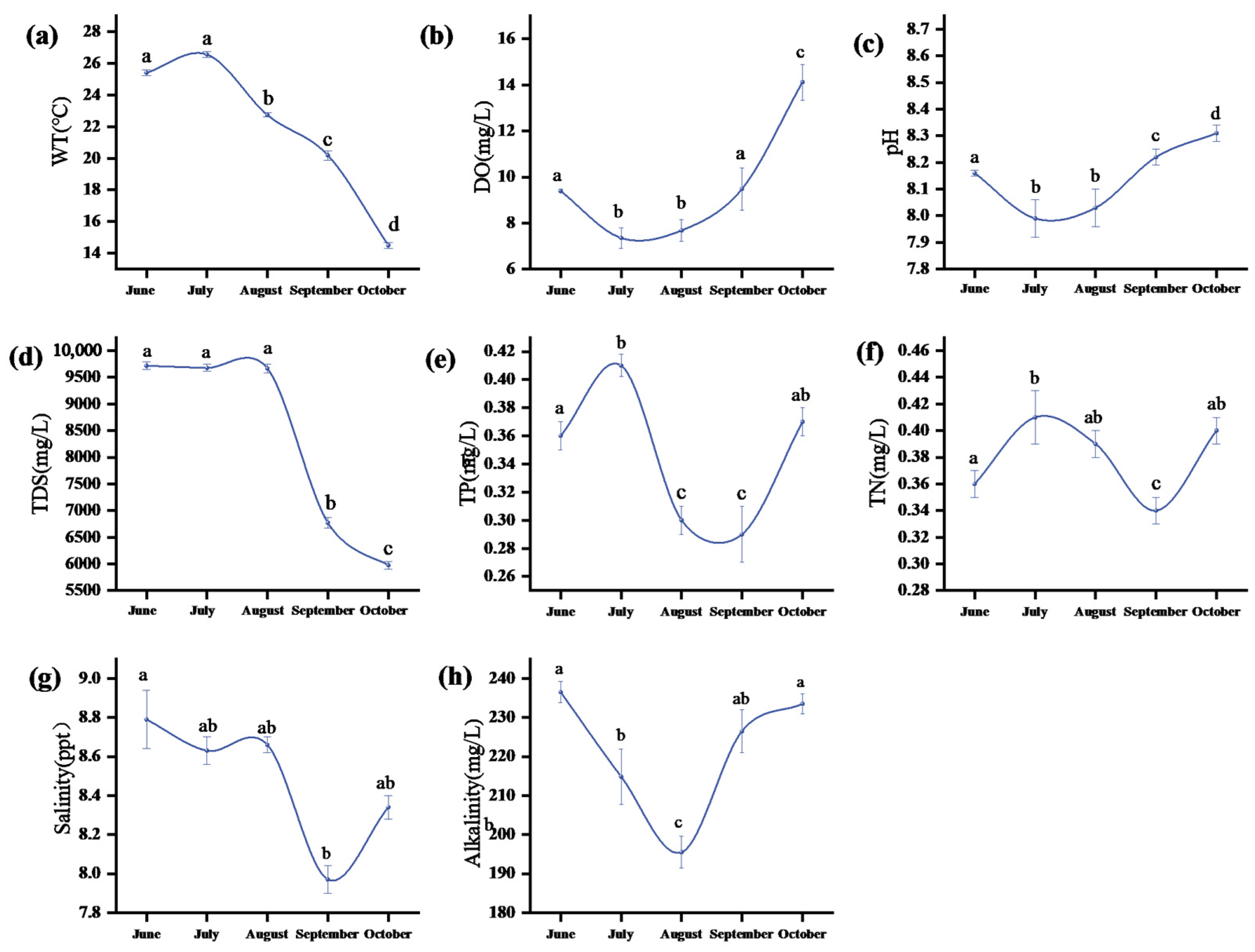
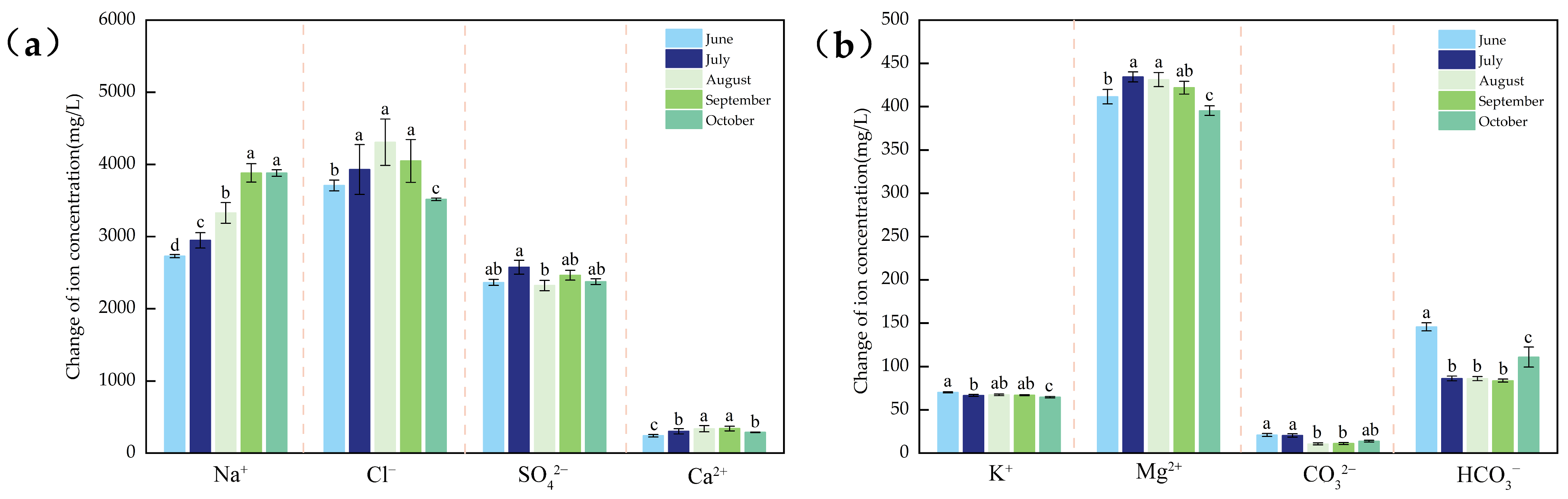
3.1. Physical and Chemical Indicators of Water Body

Figure 2 shows the seasonal variations in the physicochemical indicators of water at the sampling points. The water temperature (WT) fluctuated between 14.5 °C and 26.56 °C. The water temperature increased in June (with an average value of 25.41 ± 0.20 °C) and peaked in July (26.56 ± 0.19 °C). There was no significant difference between June and July (ANOVA, p > 0.05), but it was significantly higher than that from August to October (p < 0.05). It dropped to the lowest value in October (14.50 ± 0.18 °C). The average concentration of dissolved oxygen (DO) was 9.60 mg/L, showing a trend of first decreasing and then increasing. The DO concentration was significantly the lowest in July (7.35 ± 0.45 mg/L; p < 0.05) and reached a peak of 14.12 ± 0.78 mg/L in October, with a significant difference from June (p < 0.05). The pH value ranged from 7.99 to 8.31, showing weakly alkaline conditions overall. It was the lowest in July (7.99 ± 0.07) and the highest in October (8.31 ± 0.03), and the difference between the two was extremely significant (p < 0.01). The TDS concentration varied between 5975.30 and 9715.75 mg/L. The concentration was the highest in June (9715.75 ± 71.30 mg/L), and it decreased significantly to 6774.20 ± 95.38 mg/L in September (p < 0.05), reaching the lowest value of 5975.30 ± 69.57 mg/L in October.

The total nitrogen (TN) concentration ranged from 0.36 to 0.41 mg/L, peaking in July (0.41 ± 0.02 mg/L), which was significantly higher than the September minimum (p < 0.05). Total phosphorus (TP) concentrations varied between 0.29 and 0.41 mg/L, reaching their maximum in July (0.41 ± 0.01 mg/L) and showing significant differences from the September minimum (0.29 ± 0.02 mg/L; p < 0.01). Salinity ranged from 7.94 to 8.79 ppt, with June values (8.79 ± 0.15 ppt) being significantly higher than September minima (7.97 ± 0.07 ppt; p < 0.05). Alkalinity (ALK, as CaCO₃) varied between 195.48 and 236.54 mg/L, peaking in June (236.54 ± 2.69 mg/L), decreasing significantly to its lowest level in August (195.48 ± 4.05 mg/L; p < 0.01), and recovering to 233.51 ± 2.56 mg/L by October.

Cation concentration analysis (Figure 3) revealed that the saline–alkaline water bodies exhibited the following characteristics: Na⁺ > Mg²⁺ > Ca²⁺ > K⁺. The Mg²⁺ concentration peaked in July (434.42 ± 5.91 mg/L), showing significantly higher values than October (395.48 ± 5.52 mg/L; p < 0.01). Ca²⁺ concentrations ranged between 242.03 and 341.84 mg/L with minimal monthly variation across sampling sites. September showed the highest values (341.84 ± 33.13 mg/L), significantly exceeding June levels (242.03 ± 18.10 mg/L; p < 0.01). As the least concentrated cation, K⁺ concentration occurred in June (70.31 ± 0.58 mg/L), while August recorded the lowest values (67.36 ± 0.88 mg/L; p < 0.05).

Anion concentration analysis revealed the following order: Cl⁻ > SO₄²⁻ > HCO₃⁻ > CO₃²⁻. Cl⁻ concentrations varied from 3516.16 to 4309.11 mg/L, peaking in August (4309.11 ± 321.41 mg/L) and showing significant differences from October minima (3516.16 ± 18.11 mg/L; p < 0.05). The SO₄²⁻ concentration ranged from 2321.37 to 2575.50 mg/L, with July maxima (2575.50 ± 96.72 mg/L) being significantly higher than August values (2321.37 ± 70.37 mg/L; p < 0.05). HCO₃⁻ concentrations ranged from 83.84 to 145.74 mg/L, with June peaks (145.74 ± 4.70 mg/L) differing significantly from the July–September values (p < 0.05). CO₃²⁻ concentrations varied between 10.78 and 20.51 mg/L, with June maxima (21.06 ± 1.62 mg/L) showing highly significant differences from August minima (10.78 ± 1.19 mg/L; p < 0.01). Overall, ion concentrations followed an initial increase followed by a decreasing trend.

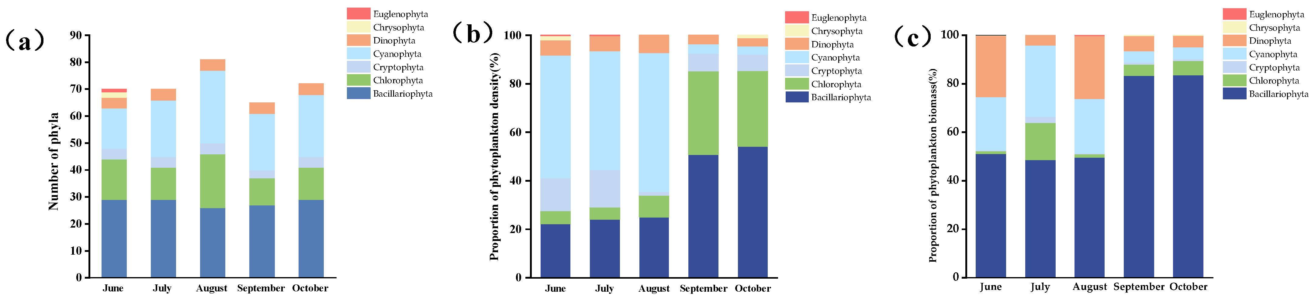
3.2. Taxonomic Composition of Phytoplankton

Microscopic examination identified a diverse phytoplankton community consisting of 115 taxonomic units, distributed across 47 genera and seven phyla. The taxonomic composition was as follows: Bacillariophyta (48 taxa), Cyanophyta (32 taxa), Chlorophyta (23 taxa), Dinophyta (5 taxa), Cryptophyta (4 taxa), Chrysophyta (2 taxa), and Euglenophyta (1) (Figure 4a). In June, a total of 70 phytoplankton taxa spanning seven phyla were recorded. Bacillariophyta were the most abundant group, comprising 29 taxa (41.42% of the total). Cyanophyta and Chlorophyta accounted for 15 (21.42%) and 12 taxa (17.14%), respectively, while Dinophyta and Cryptophyta each contributed 4 taxa (5.70%). The phylum Chrysophyta and the phylum Euglenophyta have two and one taxonomic units, respectively, accounting for approximately 2.86% and 1.43% of the total number. During July, a similar taxa richness was observed, with 70 phytoplankton taxa identified. Bacillariophyta remained the dominant group, representing 29 taxa (41.40%). Cyanophyta and Chlorophyta constituted 21 (30%) and 12 taxa (17.14%), respectively, and Cryptophyta and Dinophyta each comprised 4 taxa (5.71%). August exhibited the highest phytoplankton diversity, with 81 taxa identified across five phyla. Cyanophyta and Bacillariophyta were the dominant taxa, representing 27 (33.33%) and 26 taxa (32.09%), respectively. Chlorophyta contributed 20 taxa (24.69%), while Dinophyta and Cryptophyta each accounted for 4 taxa (4.93%). In September, 65 phytoplankton taxa from five phyla were documented. Bacillariophyta (27 taxa, 41.53%) and Cyanophyta (21 taxa, 32.30%) were the most abundant groups. Chlorophyta, Dinophyta, and Cryptophyta represented 10 (15.38%), 4 (6.15%), and 3 taxa (4.61%), respectively. By October, as water temperatures (WT) decreased, Bacillariophyta continued to dominate, comprising 29 taxa (40.27%). Despite the decline in WT, the average temperature in the high-salinity–alkaline lake remained at approximately 14 °C. Cyanophyta followed with 23 taxa (31.94%), Chlorophyta with 12 taxa (16.66%), and Dinophyta and Cryptophyta each with 4 taxa (5.55%) (see Supplementary Table S1).

3.3. The Relative Density and Relative Biomass of Phytoplankton

The monthly variations in the relative density and biomass of phytoplankton in the saline–alkaline lake are presented in Figure 4b,c. In June, the phytoplankton density peaked, reaching 53.54 × 10⁷ cells/L, of which Cyanophyta dominated, accounting for 57.23% of the total density. Bacillariophyta and Cryptophyta accounted for 22.27% and 13.60%, respectively, of the total density. In July, the total phytoplankton density reached 27.32 × 10⁷ cells/L, with the community dominated by Cyanophyta (13.39 × 10⁷ cells/L, 49.02%), followed by Bacillariophyta (6.59 × 10⁷ cells/L, 24.12%) and Cryptophyta (4.23 × 10⁷ cells/L, 15.47%), while other phyla collectively accounted for 11.39% of the total density. In August, the total phytoplankton density reached 31.68 × 10⁶ cells/L. The community was dominated by Cyanophyta (16.68 × 10⁶ cells/L, accounting for 52.66%), followed by Bacillariophyta (5.79 × 10⁶ cells/L, 18.28%), Chlorophyta (4.34 × 10⁶ cells/L, 13.71%), and Dinophyta (3.35 × 10⁶ cells/L, 10.57%). Cryptophyta constituted 4.78% (1.52 × 10⁶ cells/L) of the total. Compared to August, the total phytoplankton density in September decreased to 27.64 × 10⁵ cells/L, while the relative proportions of Bacillariophyta (12.69 × 10⁵ cells/L) and Chlorophyta (8.49 × 10⁵ cells/L) increased to 45.9% and 30.7%, respectively. In October, the total phytoplankton density was 23.76 × 10⁵ cells/L, with Chlorophyta density reaching 7.43 × 10⁵ cells/L (31.29% of total density), second only to Bacillariophyta (11.48 × 10⁵ cells/L, 54.2%).

Through comparative analysis, the changes in the phytoplankton biomass from June to October significantly varied. The total phytoplankton biomass between months ranged from 0.20 × 10⁻¹ to 3.4 × 10⁻¹ mg/L (Figure 4c). A progressive increase was observed from June (0.12 mg/L) to July (0.14 mg/L) and August (0.21 mg/L). The peak biomass (0.34 mg/L) occurred in September, followed by a sharp decline to the lowest level (0.10 mg/L) in October. Notably, during September–October, as water temperature gradually decreased, the biomass of Bacillariophyta increased significantly, accounting for 75.51% (September) and 73.33% (October) of the total phytoplankton biomass, establishing them as the dominant taxonomic group during this period.

3.4. Diversity Index Analysis

From June to October, the Pielou’s evenness index varied between 0.69 and 0.81. It reached its peak in July, with a value of 0.80, and its lowest value in August, at 0.69. A statistical analysis demonstrated that the Pielou’s evenness index in August differed extremely significantly from those in June and July (p < 0.001), and significantly from that in October (p < 0.01) (Figure 5a). The Margalef’s richness index ranged from 2.35 to 4.11, with no significant differences observed among months (p > 0.05) (Figure 5b). Regarding the Shannon–Wiener index of phytoplankton communities in the saline–alkaline lake, values ranged from 2.91 to 3.81. ANOVA indicated significant differences among months (ANOVA, p < 0.05). Specifically, the value in June was significantly higher than those in July and October (p < 0.01), while the value in August was significantly lower than those in June and September (p < 0.05) (Figure 5c).

3.5. Dominant Phytoplankton Taxa

From June to October 2023, a total of eight dominant phytoplankton species (Y ≥ 0.02) were identified at the 10 sampling sites, and the dominance varied between 0.02 and 0.15. The phytoplankton community in the saline–alkaline lake mainly comprised Bacillariophyta, Cyanophyta, Chlorophyta, and Cryptophyta. In June, the dominant species were Microcystis spp. (0.15), Merismopedia sp. (0.12), Chroomonas acuta (0.05), Gymnodinium aeruginosum (0.05), Chlorella sp. (0.04), Cyclotella spp. (0.04), and Cyclotella meneghiniana (0.04). In July, Microcystis spp. (0.14) dominated, while Chlorella sp. (0.04), Cyclotella spp., and Cyclotella meneghiniana all exhibited a dominance value of 0.03. Microcystis spp. continued to dominate in August. In September, both Cyclotella meneghiniana and Microcystis spp. attained a value of 0.04. In October, the abundance of Cyclotella meneghiniana (0.06), Navicula cryptocephala (0.05), Cyclotella sp., Chlorella sp., and Chroomonas acuta all reached approximately 0.03 (

Table 2. Dominant taxa and the dominance of phytoplankton in Swan Lake from June to October.

Phylum	Genus	Dominant Taxa	June	July	August	September	October
Bacillariophyta	Cyclotella	Cyclotella spp.	0.04	0.03	-	-	0.03
	Cyclotella	Cyclotella meneghiniana	0.04	-	0.04	0.04	0.06
Cyanophyta	Merismopedia	Merismopedia sp.	0.12	0.03	-	-	-
	Microcystis	Microcystis spp.	0.15	0.14	0.12	0.04	-
Chlorophyta	Chlorella	Chlorella sp.	0.04	0.04	0.04	-	0.03
Cryptophyta	Chroomonas	Chroomonas acuta	0.05	-	-	-	0.03
	Navicula	Navicula cryptocephala	-	-	0.03	-	0.05
Dinophyta	Peridinium	Gymnodinium aeruginosum	0.05	-	-	-	-

Note: The ′-′ in the table indicates that the phytoplankton dominance Y in this month did not reach 0.02, that is, the non-dominant taxa.

).

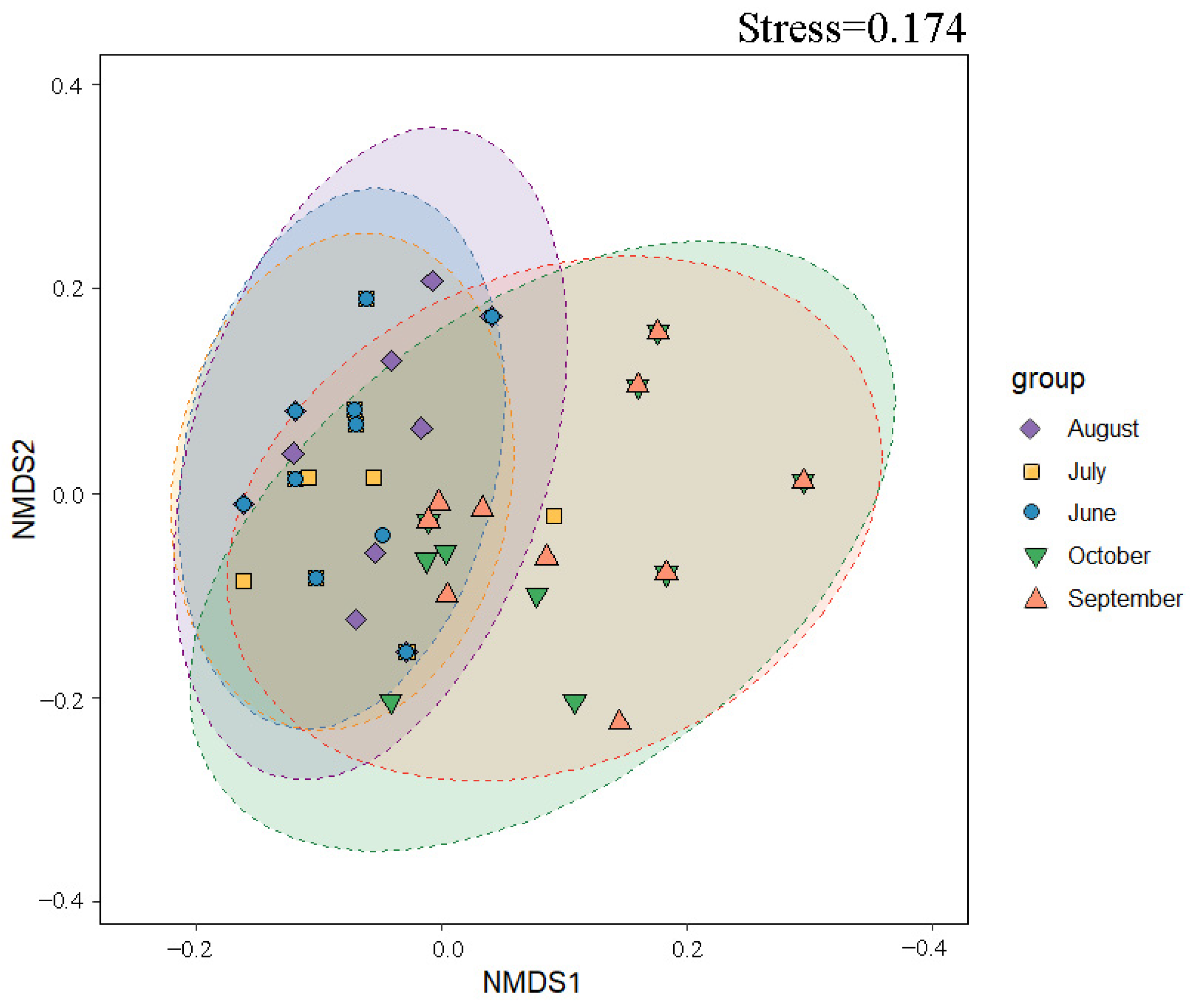
3.6. Analysis of Phytoplankton Community Structure Characteristics

The NMDS (non-metric multidimensional scaling) analysis effectively captured community dissimilarities among samples, where closer proximity between points indicates greater similarity in species composition. As shown in Figure 6, significant spatial heterogeneity was observed in phytoplankton community structure across the 50 sampling sites. Data points for June, July, and August exhibited partial overlap, suggesting shared species composition or analogous ecological attributes among these months. In contrast, September samples showed greater dispersion in the ordination space, with a distinct separation trend from other groups but partial overlap with October, implying transitional similarity in community structure between these two months. PERMANOVA tests further confirmed statistically significant temporal variations in community composition from June to October (R² = 0.422, p < 0.001), highlighting distinct ecological features between early and late sampling periods.

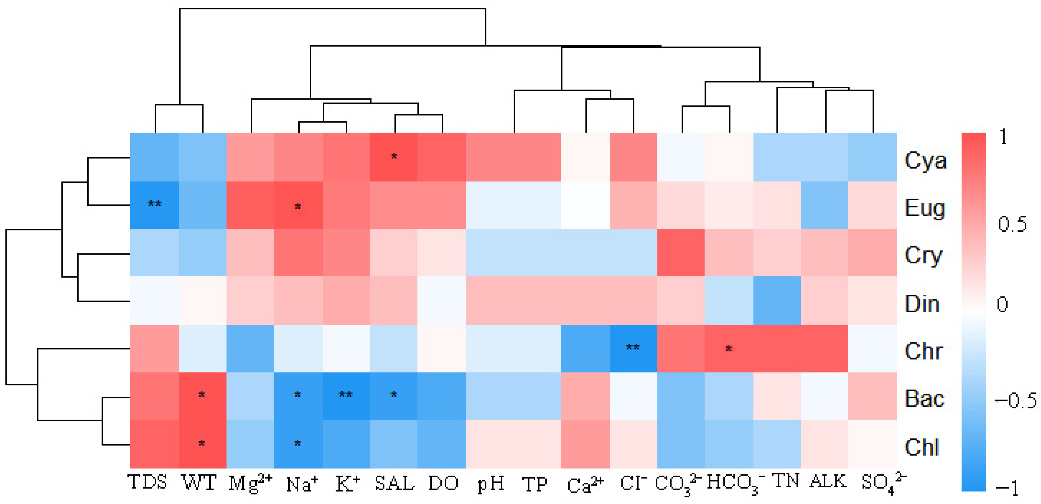
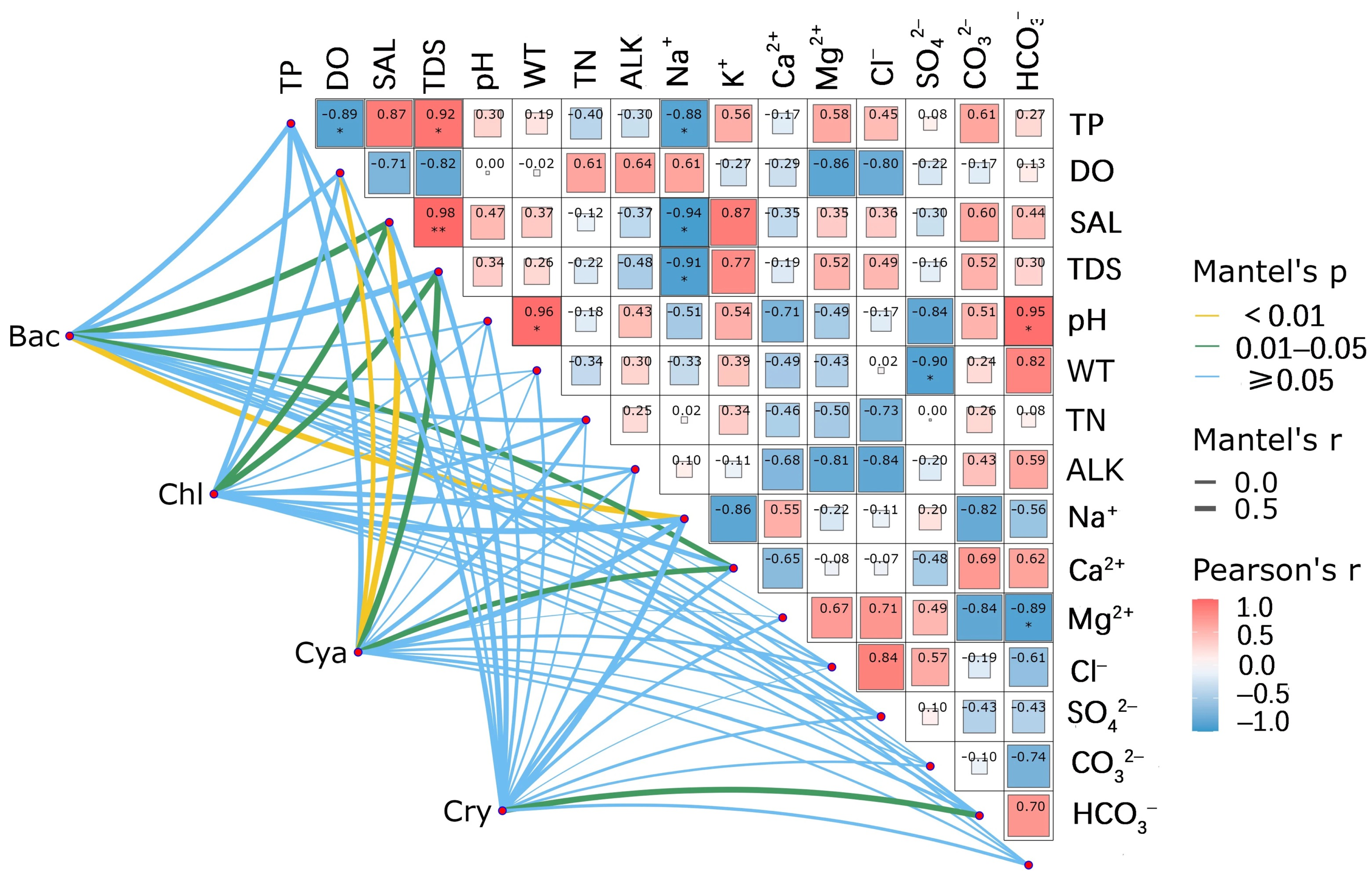
3.7. Correlation Analysis Between the Phytoplankton Community and Environmental Factors

Spearman correlation analysis revealed that salinity, WT, Na⁺, TDS, HCO₃⁻, Cl⁻, and K⁺ were key environmental factors significantly influencing phytoplankton community structure (Figure 7). Cyanophyta showed a significantly positive correlation with salinity (ρ = 0.90, p < 0.05); Euglenophyta exhibited a significantly positive correlation with Na⁺ concentration (ρ = 0.87, p < 0.05), while demonstrating an extremely significant negative correlation with TDS (ρ = −0.97, p < 0.01). Cryptophyta displayed no significant correlations with environmental factors (p > 0.05) but showed relatively strong non-significant associations with CO₃²⁻ (ρ = 0.79), Na⁺ (ρ = 0.72), and K⁺ (ρ = 0.61). Dinophyta had no significant correlations with any environmental factors (p > 0.05). Chrysophyta was significantly positively correlated with HCO₃⁻ (ρ = 0.83, p < 0.05) and extremely significantly negatively correlated with Cl⁻ (ρ = −0.95, p < 0.01). Bacillariophyta showed a significantly We appreciate your input. All statistical notations have been corrected: Spearman’s ρ and p-values are now consistently italicized (e.g., ρ = 0.87, p < 0.05).positive correlation with WT (ρ = 0.91, p < 0.05) and significantly negative correlations with Na⁺ (ρ = −0.89, p < 0.05), salinity (ρ = −0.90, p < 0.05), and K⁺ (ρ = −0.91, p < 0.01). Chlorophyta was significantly positively correlated with WT (ρ = 0.90, p < 0.05) and significantly negatively correlated with Na⁺ concentration (ρ = −0.88, p < 0.05).

In the Mantel test, only the four phyla of phytoplankton, namely Bacillariophyta, Chlorophyta, Cyanophyta, and Cryptophyta, were selected for analysis. This is because the abundances of the remaining phytoplankton phyla were extremely low. Such low abundances could easily lead to biases in the Mantel test, which is sensitive to sample size and data distribution, and thus fail to ensure the reliability of the results. Figure 8 shows that during the period from June to October, there is a significant positive correlation between pH and SAL in the phytoplankton community of saline–alkali lakes (p < 0.05). Further analysis indicates that the total density of diatoms is significantly positively correlated with SAL, TDS, K⁺, and Na⁺ (Mantel test, p < 0.05). Similarly, the total density of green algae exhibits a significant positive correlation with SAL and TDS (Mantel test, p < 0.05). The total density of Cyanophyta is significantly positively correlated with dissolved oxygen (DO) concentration (Mantel test, p < 0.01), SAL (Mantel test, p < 0.01), TDS (Mantel test, p < 0.05), and K⁺ (Mantel test, p < 0.05), while the correlations with other environmental factors are not significant (p > 0.05). In addition, the total density of Cryptophyta is significantly positively correlated with CO₃²⁻ (Mantel test, p < 0.05).

This study employed a redundancy analysis (RDA) to examine how environmental factors determine phytoplankton community structure (Figure 9). Initial preprocessing eliminated six collinear variables (Ca²⁺, Mg²⁺, TP, DO, SO₄²⁻, CO₃²⁻) based on VIF < 10 criteria. Monte Carlo permutation tests (n = 999) identified the following six key drivers: WT (p < 0.001, F = 14.99), TDS (p < 0.01, F = 14.19), pH (p < 0.05, F = 13.01), alkalinity (p < 0.05, F = 12.91), salinity (p < 0.05, F = 1.93), and Na⁺ (p < 0.05, F = 2.73). The RDA indicated that the phytoplankton community exhibited certain heterogeneity among months, showing distinct seasonal succession characteristics; samples from June to July were mainly distributed in the second and third quadrants, those in August clustered towards the third quadrant, while samples in September and October were located in the first and fourth quadrants, respectively. The first two ordination axes accounted for 87.3% of the total community variation, with Axis 1 explaining 68.3% and Axis 2 contributing 19.0%. A species–environment analysis showed that Microcystis spp. and Chroomonas acuta correlated positively with salinity, HCO₃⁻, K⁺, TDS, and WT, while Cyclotella spp. and Merismopedia spp. correlated negatively with pH and TN. Conversely, Navicula cryptocephala, Cyclotella meneghiniana, Gymnodinium spp., and Chlorella spp. exhibited positive relationships with Na⁺ and alkalinity but negative correlations with TDS and WT.

4. Discussion

4.1. Characteristics of the Phytoplankton Community Structure

Saline–alkaline land areas are widely distributed in northwest China, and their ecological environments are influenced by multiple factors, such as drought, scarce precipitation, and notable diurnal temperature variations [46,47]. To improve these saline–alkaline lands, an innovative strategy of using fisheries to manage salinity has been adopted locally, thereby utilizing saline–alkaline water resources. The spatio-temporal variations in the phytoplankton community structure are significant. A total of seven phyla, 47 genera, and 115 taxa of phytoplankton were identified, with Cyanophyta and Bacillariophyta dominating the region, which is consistent with previous research findings [48] and verifies the seasonal succession patterns in this area. Different regions exhibit distinct community characteristics; for example, Chlorophyta and Bacillariophyta dominate in Qinghai [49]. In contrast, northeastern China exhibits unique community features, with Chlorophyta and Bacillariophyta dominating in the spring and autumn [50]; although the abundance of Cyanophyta increases in summer, it does not become dominant, mainly because of differences in the growth characteristics and habitat adaptability of phytoplankton [51].

Changes in phytoplankton are strongly influenced by the salt composition and salt content in lakes, and these ionic compositions are mainly controlled by the water supply and drainage methods and regional environmental differences [52]. In the Alar region of the arid region in northwest China, the Tarim River is the main river, and its water source largely depends on ice and snow meltwater and groundwater recharge from the Tianshan Mountains and Kunlun Mountains [53]. The wide distribution of saline–alkaline land and arid climatic conditions result in highly variable water chemistry in this area [54]. Meanwhile, in northwestern Gansu and Ningxia, the salinity of lakes is generally high, creating a distinct saline–alkaline environment, which is conducive to the survival and reproduction of diatoms and cyanobacteria species. Through adaptive evolution, they exhibit ecological advantages under high-salinity conditions [55]. In contrast, Northeast China exhibits different water characteristics due to seasonal freezing and thawing and agricultural irrigation. The salinity of subsurface water gradually increases in winter and peaks in spring when ice melts. Moreover, agricultural irrigation activities increase the content of nitrate (NO₃⁻) and phosphate (PO₄³⁻) in water, and these changes further affect the structure of the phytoplankton community [56]. Notably, the salt composition of lakes in Ningxia is more significantly affected by the interaction between groundwater and surface water. The proportions of sulfate and chloride are relatively high, which imposes a specific effect on the phytoplankton community [57,58]

This study has found that, in the saline–alkali lake ecosystem, the density of phytoplankton reaches its peak in June. According to statistics, the density order is June > July > August > September > October. In June, the water temperature of the saline–alkali lake is approximately 24.51 °C, which is extremely favorable for the growth of Cyanophyta. This is consistent with the dominance of Cyanophyta during this period [59]. Cyanophyta species, such as Microcystis, exhibit growth advantages in high-temperature and high-salinity environments in summer. This may cause blooms and pose a threat to the water quality and aquatic ecosystems [60]. In August, Alar City enters the rainy season and the farmland irrigation season. Rainwater and irrigation water become the main sources of recharge for the saline–alkali lake. This change has multiple impacts on the phytoplankton, as follows: The influx of a large amount of rainwater increases the water volume of the lake, diluting the nutrient salt concentration and reducing the density of phytoplankton. The clouds during the rainy season weaken the light, inhibiting the photosynthesis of phytoplankton and further reducing the biomass [61]. In addition, the unique environment of the saline–alkali lake leads to a high proportion of sulfate and chloride in the lake salt, which is related to the aridity and high evaporation in the region [62]. In October, the water temperature of the saline–alkali lake drops to 14.50 °C. Due to the fact that cyanobacteria are intolerant of low temperatures and their growth and reproduction are restricted [63,64], while chlorophyta and bacillariophyta still maintain physiological activity at low temperatures, the relative densities of chlorophyta and bacillariophyta increase, and the density proportion of cyanobacteria decreases.

4.2. Relationships Between Phytoplankton and Environmental Factors

In lake ecosystems, phytoplankton community composition and distribution are regulated by multiple environmental factors like WT, salinity, TN, TP, and pH. Their effects vary among different water bodies [65].

Water temperature (WT) is a key factor influencing the distribution of phytoplankton species [66,67,68]. Spearman correlation analysis revealed significant positive correlations between WT and both Bacillariophyta and Chlorophyta (p < 0.05). WT directly regulates phytoplankton growth rates by influencing algal cellular growth, reproduction, and metabolic functions [69]. Previous studies have demonstrated that Cyanobacteria exhibit optimal growth at temperatures above 25 °C, while Bacillariophyta thrive better in cooler waters, and Chlorophyta prefer warmer habitats [70]. Temporally, the October water temperature (14.5 °C) in the saline–alkaline lake was below the optimal growth range (25–35 °C) for both Cyanobacteria and Chlorophyta, which explains the dominance of Bacillariophyta during this period. Notably, during June–August, precipitation recharge during the rainy season in the Alar region diluted nutrient concentrations in the lake water, while increased cloud cover led to reduced light availability, both of which significantly influenced phytoplankton biomass. As a result, this also leads to changes in the composition of phytoplankton species and dominant populations [71]. This phenomenon exhibits variations across different aquatic systems; for example, in saline–alkaline lakes in Northeast China, an increase in WT results in a shift in the dominant population from Bacillariophyta to Cyanophyta; whereas, in the coastal waters of the Antarctic Peninsula, the dominant population shifts from diatoms to cryptophytes [72]. In saline–alkaline lakes in Alar, Xinjiang, an increase in WT leads to an increase in the number of phytoplankton, primarily due to more favorable growth conditions and additional nutrients provided by rising groundwater levels or supplementary water sources from the surrounding area [73].

An analysis of nutrient dynamics shows that TN and TP concentrations increase in June, decline from July to September, and rise again in October. This is likely linked to agricultural activities in the Tarim River Irrigation District. During the July–August crop water–demand peak, irrigation drainage dilutes nutrients. After September harvest, rainfall and alkali drainage canals wash residual fertilizers into the water, raising TN and TP. Summer phytoplankton absorption and denitrification also contribute to TN decrease. High summer temperatures accelerate dissolved oxygen consumption. Low dissolved oxygen prevents nitrite from being quickly oxidized to nitrate, causing nitrite accumulation. Then, nitrifying bacteria carry out denitrification, increasing N₂O release [74].

The Mantel test indicates that salinity, TDS, and K⁺ are key drivers of the phytoplankton community structure. The significant June–August TDS increase reflects the arid region’s hydrological features. In the extremely arid Alar area, water bodies concentrate, exponentially raising TDS as ion (Na⁺, Cl⁻, SO₄²⁻) concentrations multiply. However, after September, glacial meltwater recharge dilutes TDS. Bacillariophyta-wide TDS adaptability allows them to become dominant over Cyanophyta and Chlorophyta from September to October. Besides water temperature, rising TDS is an important factor in this shift [75].

An increase in the salinity can inhibit the growth of salinity-sensitive phytoplankton [76]. However, certain species of green and blue–green algae with high salt tolerance can maintain their normal physiological functions in high-salinity environments, thereby exhibiting a clear competitive advantage [77]. With an increasing salinity gradient, the number of phytoplankton species and biodiversity decrease [78]. Additionally, studies have revealed that an increase in the salinity can negatively impact the diversity and abundance of diatoms in sediments [79]. Notably, Mantel’s test analysis results revealed a significant positive correlation between the salinity and the community composition of blue–green algae, diatoms, and green algae, strongly suggesting a crucial role of salinity in driving these community structural changes.

In the studied saline–alkaline lake, salinity fluctuated from 7.94 to 8.79 ppt. From June to August, it remained stable as high-salinity agricultural drainage via alkali discharge channels offset precipitation-induced dilution. This favored salt-tolerant phytoplankton, like Chlorophyta, Cyanobacteria, and Bacillariophyta. In September, more glacial meltwater and less agricultural drainage lowered salinity, allowing salt-sensitive species to grow. By October, reduced inflow and evaporative concentration increased salinity, enabling Bacillariophyta and Cyanobacteria to dominate again due to their high salt tolerance. These trends show salinity’s seasonal filtering effect on phytoplankton community composition.

pH is also regarded as an important factor influencing the phytoplankton community structure [80]. The results of the Mantel test verify that there is a positive correlation between the pH value and the abundances of diatoms, cyanobacteria, green algae, and cryptophytes. In the study area, alkaline water bodies with a pH ranging from 7.99 to 8.31 have relatively high algal productivity, and the alkaline environment is more conducive to the photosynthesis of phytoplankton. The wetland of the saline–alkaline lake in Alar is surrounded by deserts with low vegetation coverage. It mainly depends on the recharge of agricultural irrigation drainage water. Most of the area is covered by saline–alkaline aeolian soil. The ecological water transfer and strong evaporation in the arid region have led to the salinization and alkalization of the wetland’s soil and water, causing the pH of the water body to increase from September to October.

The pH fluctuations directly impact nutrient forms. For instance, phosphorus dissolves in acidic water but precipitates in alkaline conditions, affecting phytoplankton’s phosphorus absorption and utilization [81]. pH and salinity interact to shape phytoplankton community distribution and composition [82]. In high-salinity and high-pH settings, salt-tolerant phytoplankton thrive, while low-salinity and low-pH conditions favor other phytoplankton types [83].

In addition, an increase in the HCO₃⁻ concentration provides a rich carbon source for photosynthetic organisms such as cyanobacteria and alters the structure of the phytoplankton community by affecting the stability of the pH value [84]. In saline–alkaline water, Mg²⁺ is a key component of chlorophyll, and its appropriate presence can promote phytoplankton growth, because it provides a sufficient source of magnesium to support photosynthesis [85]. However, excessive Mg²⁺ levels, especially when cooccurring with high concentrations of other ions (such as Na⁺ and Cl⁻), may interfere with and inhibit the absorption and utilization of other important nutrients (such as K⁺, Ca²⁺, and P), thus adversely affecting phytoplankton growth. Hence, balanced regulation of the Mg²⁺ concentration is particularly critical in saline–alkaline water ecosystems [86].

The phytoplankton community in the saline–alkali lake is regulated by both the grazing of zooplankton and human activities. Cladocerans (such as Daphnia) selectively feed on small green algae and cryptophytes, indirectly promoting the dominance of diatoms. Rotifers, on the other hand, influence the community succession by feeding on cyanobacteria. In the future, it is necessary to combine zooplankton data to evaluate the relative contributions of bottom-up control (nutrients) and top-down control (grazing).

As a typical agricultural irrigation area, Alar has pesticide residues in the agricultural drainage water input, which further alters the competitive pattern. This inhibits sensitive diatoms and promotes the growth of pollution-tolerant Cyanophyta (such as Microcystis). The interactive effects of these anthropogenic disturbance factors and natural environmental factors (such as salinity and water temperature) further increase the complexity of the dynamics of the phytoplankton community in the saline–alkali lakes in arid regions [87]. The study found that Microcystis and Cyclotella meneghiniana have a relatively high occurrence frequency among the phytoplankton in the saline–alkali lake and are absolute dominant species. Therefore, it is necessary to strengthen the long-term monitoring of the population density, the dynamic changes of these species, and the water environmental quality status. Future research should prioritize the development of salt-tolerant algal strain selection and intelligent regulation technologies to comprehensively enhance the adaptability and stability of saline–alkaline ecosystems.

5. Conclusions

Through an investigation of highly saline–alkaline lakes and ponds in Xinjiang, northwest China, we identified 115 taxa of phytoplankton belonging to seven phyla, revealing their diversity and seasonal dynamics. The phytoplankton community exhibited significant seasonal variations, with Cyanophyta, Bacillariophyta, and Chlorophyta dominating from June to August, while the dominance of Bacillariophyta and Chlorophyta increased in October. Key species, such as Microcystis spp., Merismopedia sp., and Cyclotella meneghiniana, played crucial roles in maintaining community stability.

Spearman correlation analysis revealed that salinity, WT, Na⁺, TDS, HCO₃⁻, Cl⁻, and K⁺ were key environmental factors significantly influencing phytoplankton community structure. RDA results indicated that WT, TDS, alkalinity, pH, salinity, and Na⁺ were the key factors driving seasonal variations in phytoplankton communities. This study provides reference data for improving saline–alkaline environments through fisheries, aiming to enhance aquaculture efficiency and enrich the biodiversity data of saline–alkaline lakes. In the future, we will delve deeply into the ecological functions of phytoplankton communities and their interactions with environmental factors. By implementing precise ecological restoration strategies, such as habitat rehabilitation, biodiversity conservation, and sustainable resource management, we aim to promote the sustainable development of ecological fisheries in saline–alkaline lakes in northwest China. This will provide scientific support for the conservation and utilization of similar ecosystems globally.

References

1. Yan, H.U.; Fan, Y.; Ning, Y.; Wei, J.; Yong, C. Analysis and prospects of saline-alkali land in China from the perspective of utilization. Chin. J. Soil Sci. 2023, 54, 489–494. [Google Scholar]
2. Yang, J.; Zhang, S.; Li, Y.; Bu, K.; Zhang, Y.; Chang, L.; Zhang, Y. Dynamics of saline-alkali land and its ecological regionalization in western Songnen plain, China. Chin. Geogr. Sci. 2010, 20, 159–166. [Google Scholar] [CrossRef]
3. Zhou, Y.; Li, Y.; Li, W.; Li, F.; Xin, Q. Ecological responses to climate change and human activities in the arid and semi-arid regions of Xinjiang in China. Remote Sens. 2022, 14, 3911. [Google Scholar] [CrossRef]
4. Wang, F.; Chen, X.; Luo, G.; Han, Q. Mapping of regional soil salinities in Xinjiang and strategies for amelioration and management. Chin. Geogr. Sci. 2015, 25, 321–336. [Google Scholar] [CrossRef]
5. Cuevas, J.; Daliakopoulos, I.N.; Del Moral, F.; Hueso, J.J.; Tsanis, I.K. A review of soil-improving cropping systems for soil salinization. Agronomy 2019, 9, 295. [Google Scholar] [CrossRef]
6. Fang, S.; Tu, W.; Mu, L.; Sun, Z.; Hu, Q.; Yang, Y. Saline alkali water desalination project in southern Xinjiang of China: A review of desalination planning, desalination schemes and economic analysis. Renew. Sustain. Energy Rev. 2019, 113, 109268. [Google Scholar] [CrossRef]
7. Wang, X.; Zhu, H.; Hou, S.; Cui, H.; Yan, B. Environmental impacts of fertilization during rice production in saline-alkali paddy fields based on life cycle assessment. J. Clean. Prod. 2024, 467, 142947. [Google Scholar] [CrossRef]
8. Yu, Y.; Yu, R.; Chen, X.; Yu, G.; Gan, M.; Disse, M. Agricultural water allocation strategies along the oasis of Tarim River in northwest China. Agric. Water Manag. 2017, 187, 24–36. [Google Scholar] [CrossRef]
9. Li, Q.; Zhou, J.; Zhou, Y.; Bai, C.; Tao, H.; Jia, R.; Ji, Y.; Yang, G. Variation of groundwater hydrochemical characteristics in the plain area of the Tarim Basin, Xinjiang region, China. Environ. Earth Sci. 2014, 72, 4249–4263. [Google Scholar] [CrossRef]
10. Belovsky, G.E.; Stephens, D.; Perschon, C.; Birdsey, P.; Paul, D.; Naftz, D.; Baskin, R.; Larson, C.; Mellison, C.; Luft, J.; et al. The Great Salt Lake ecosystem (Utah, USA): Long term data and a structural equation approach. Ecosphere 2011, 2, art33. [Google Scholar] [CrossRef]
11. Pálmai, T.; Szabó, B.; Kotut, K.; Krienitz, L.; Padisák, J. Ecophysiology of a successful phytoplankton competitor in the African flamingo lakes: The green alga Picocystis salinarum (picocystophyceae). J. Appl. Phycol. 2020, 32, 1813–1825. [Google Scholar] [CrossRef]
12. Laplace-Treyture, C.; Derot, J.; Prévost, E.; Le Mat, A.; Jamoneau, A. Phytoplankton morpho-functional trait dataset from French water-bodies. Sci. Data 2021, 8, 40. [Google Scholar] [CrossRef] [PubMed]
13. Hallegraeff, G.M. Ocean climate change, phytoplankton community responses, and harmful algal blooms: A formidable predictive challenge. J. Phycol. 2010, 46, 220–235. [Google Scholar] [CrossRef]
14. Deppeler, S.L.; Davidson, A.T. Southern Ocean phytoplankton in a changing climate. Front. Mar. Sci. 2017, 4, 40. [Google Scholar] [CrossRef]
15. Xiao, R.; Su, S.; Ghadouani, A.; Wu, J. Spatial analysis of phytoplankton patterns in relation to environmental factors across the southern Taihu Basin, China. Stoch Environ. Res. Risk Assess. 2013, 27, 1347–1357. [Google Scholar] [CrossRef]
16. Çelekli, A.; Öztürk, B.; Kapı, M. Relationship between phytoplankton composition and environmental variables in an artificial pond. Algal Res. 2014, 5, 37–41. [Google Scholar] [CrossRef]
17. Sun, W.; Dong, S.; Jie, Z.; Zhao, X.; Zhang, H.; Li, J. The impact of net-isolated polyculture of tilapia (Oreochromis niloticus) on plankton community in saline–alkaline pond of shrimp (Penaeus vannamei). Aquacult. Int. 2011, 19, 779–788. [Google Scholar] [CrossRef]
18. de Melo Soares, R.H.; de Oliveira Fernandes, F.; de Assunção, C.A.; Borburema, H.D.; do Amaral Carneiro, M.A.; Marinho-Soriano, E. Macroalgal diversity along an environmental gradient in a saltwork. Estuar. Coast. Shelf Sci. 2023, 288, 108377. [Google Scholar] [CrossRef]
19. Zhou, B.; Liang, C.; Chen, X.; Ye, S.; Peng, Y.; Yang, L.; Duan, M.; Wang, X. Magnetically-treated brackish water affects soil water-salt distribution and the growth of cotton with film mulch drip irrigation in Xinjiang, China. Agric. Water Manag. 2022, 263, 107487. [Google Scholar] [CrossRef]
20. Kumar, M.; Chadha, N.K.; Prakash, S.; Pavan-Kumar, A.; Harikrishna, V.; Gireesh-Babu, P.; Krishna, G. Salinity, stocking density, and their interactive effects on growth performance and physiological parameters of white-leg shrimp, Penaeus vannamei (Boone, 1931), reared in inland ground saline water. Aquacult. Int. 2024, 32, 675–690. [Google Scholar] [CrossRef]
21. Anufriieva, E.V. How can saline and hypersaline lakes contribute to aquaculture development? A review. J. Oceanol. Limnol. 2018, 36, 2002–2009. [Google Scholar] [CrossRef]
22. Lymbery, A.J.; Kay, G.D.; Doupé, R.G.; Partridge, G.J.; Norman, H.C. The potential of a salt-tolerant plant (Distichlis spicata cv. nypa forage) to treat effluent from inland saline aquaculture and provide livestock feed on salt-affected farmland. Sci. Total Environ. 2013, 445–446, 192–201. [Google Scholar] [CrossRef]
23. Salunke, M.; Kalyankar, A.; Khedkar, C.D.; Shingare, M.; Khedkar, G.D. A review on shrimp aquaculture in India: Historical perspective, constraints, status and future implications for impacts on aquatic ecosystem and biodiversity. Rev. Fish. Sci. Aquacult. 2020, 28, 283–302. [Google Scholar] [CrossRef]
24. Fatima, A.; Abbas, G.; Kasprzak, R. Assessment of hydrobiological and soil characteristics of non-fertilized, earthen fish ponds in Sindh (Pakistan), supplied with seawater from tidal creeks. Water 2022, 14, 2115. [Google Scholar] [CrossRef]
25. Palmer, P.J.; Burke, M.J.; Palmer, C.J.; Burke, J.B. Developments in controlled green-water larval culture technologies for estuarine fishes in Queensland, Australia and elsewhere. Aquaculture 2007, 272, 1–21. [Google Scholar] [CrossRef]
26. Zhang, R.; Luo, L.; Wang, S.; Guo, K.; Xu, W.; Zhao, Z. Screening and characteristics of ammonia nitrogen removal bacteria under alkaline environments. Front. Microbiol. 2022, 13, 969722. [Google Scholar] [CrossRef]
27. Shang, X.; Geng, L.; Yang, J.; Zhang, Y.; Xu, W. Transcriptome analysis reveals the mechanism of alkalinity exposure on spleen oxidative stress, inflammation and immune function of Luciobarbus capito. Ecotoxicol. Environ. Saf. 2021, 225, 112748. [Google Scholar] [CrossRef]
28. Li, K.; Zhao, S.; Guan, W.; Li, K.J. Planktonic bacteria in white shrimp (Litopenaeus vannamei) and channel catfish (Letalurus punetaus) aquaculture ponds in a salt-alkaline region. Lett. Appl. Microbiol. 2022, 74, 212–219. [Google Scholar] [CrossRef]
29. Xu, C.; Su, G.; Zhao, K.; Kong, X.; Wang, H.; Xu, X.; Li, Z.; Zhang, M.; Xu, J. Societal benefits and environmental performance of Chinese aquaculture. J. Clean. Prod. 2023, 422, 138645. [Google Scholar] [CrossRef]
30. Wang, X.-N.; Gu, Y.-G.; Wang, Z.-H. Fingerprint characteristics and health risks of trace metals in market fish species from a large aquaculture producer in a typical arid province in northwestern China. Environ. Technol. Innov. 2020, 19, 100987. [Google Scholar] [CrossRef]
31. Chang, Z.-Q.; Neori, A.; He, Y.-Y.; Li, J.-T.; Qiao, L.; Preston, S.I.; Liu, P.; Li, J. Development and current state of seawater shrimp farming, with an emphasis on integrated multi-trophic pond aquaculture farms, in China—A review. Rev. Aquacult. 2020, 12, 2544–2558. [Google Scholar] [CrossRef]
32. Qiu, J.; Zhang, C.; Lv, Z.; Zhang, Z.; Chu, Y.; Shang, D.; Chen, Y.; Chen, C. Analysis of changes in nutrient salts and other water quality indexes in the pond water for largemouth bass (Micropterus salmoides) farming. Heliyon 2024, 10, e24996. [Google Scholar] [CrossRef] [PubMed]
33. Yu, R.; Wang, J. Evaluation of the environmental sustainability of farmers’ land use decisions in the saline-alkaline areas. Environ. Monit. Assess. 2015, 187, 182. [Google Scholar] [CrossRef]
34. Wang, D.; Zhang, L.; Zhang, J.; Li, W.; Li, H.; Liang, Y.; Han, Y.; Luo, P.; Wang, Z. Effect of magnetized brackish water drip irrigation on water and salt transport characteristics of sandy soil in southern Xinjiang, China. Water 2023, 15, 577. [Google Scholar] [CrossRef]
35. Zhang, J.M.; He, Z.H. Handbook of Natural Resources Survey of Inland Waters Fisheries; Agricultural Press: Beijing, China, 1991. [Google Scholar]
36. Hu, H.J.; Wei, Y.X. The Freshwater Algae of China: System, Ecology and Classification; Science Press: Beijing, China, 2006. [Google Scholar]
37. Qi, Y.Z.; Li, J.Y. Annals of Freshwater Algae in China; Science Press: Beijing, China, 2004. [Google Scholar]
38. Administration, S.E.P. Monitoring and Analysis Methods of Water and Wastewater, 4th ed.; Environmental Science Press: Beijing, China, 2002. [Google Scholar]
39. Chen, G.M. Ammonium molybdate spectrophotometric method for determination of total phosphorus in municipal sewage sludge. China Water Wastewater 2006, 22, 85–86. [Google Scholar]
40. Jouanneau, S.; Recoules, L.; Durand, M.; Boukabache, A.; Picot, V.; Primault, Y.; Lakel, A.; Sengelin, M.; Barillon, B.; Thouand, G. Methods for assessing biochemical oxygen demand (BOD): A review. Water Res. 2014, 49, 62–82. [Google Scholar] [CrossRef] [PubMed]
41. Zhao, W. Hydrobiology, 2nd ed.; China Agriculture Press: Beijing, China, 2016. [Google Scholar]
42. Grigorszky, I.; Kétyi, T.; Borics, I.; Borbély, G.; Padisák, J.; Bácsi, I.; Bánkuti, K. The effects of temperature, nitrogen, and phosphorus on the encystment of Peridinium cinctum, Stein (Dinophyta). Hydrobiologia 2006, 563, 527–535. [Google Scholar] [CrossRef]
43. Wang, X.; Sun, M.; Wang, J.; Yang, L.; Luo, L.; Li, P.; Kong, F. Microcystis genotype succession and related environmental factors in Lake Taihu during cyanobacterial blooms. Microb. Ecol. 2012, 64, 986–999. [Google Scholar] [CrossRef]
44. Gamito, S. Caution is needed when applying margalef diversity index. Ecol. Indic. 2010, 10, 550–551. [Google Scholar] [CrossRef]
45. Li, X.; Yu, H.; Wang, H.; Ma, C. Phytoplankton community structure in relation to environmental factors and ecological assessment of water quality in the upper reaches of the Genhe River in the Greater Hinggan Mountains. Environ. Sci. Pollut. Res. 2019, 26, 17512–17519. [Google Scholar] [CrossRef]
46. Li, X.; Song, Y.; Nian, F. Characteristics of water transformation and its effects on environment in the arid region. Chin. Geogr. Sci. 2000, 10, 52–60. [Google Scholar] [CrossRef]
47. Zhang, D.; Zhao, W.; Zhang, G. Soil moisture and salt ionic composition effects on species distribution and diversity in semiarid inland saline habitats, Northwestern China. Ecol. Res. 2018, 33, 505–515. [Google Scholar] [CrossRef]
48. Sui, F.; Zang, S.; Fan, Y.; Ye, H. Effects of different saline-alkaline conditions on the characteristics of phytoplankton communities in the lakes of Songnen Plain, China. PLoS ONE 2016, 11, e0164734. [Google Scholar] [CrossRef] [PubMed]
49. Li, Z.; Gao, Y.; Wang, S.; Lu, Y.; Sun, K.; Jia, J.; Wang, Y. Phytoplankton community response to nutrients along lake salinity and altitude gradients on the Qinghai-Tibet Plateau. Ecol. Indic. 2021, 128, 107848. [Google Scholar] [CrossRef]
50. Zhao, Z.; Song, T.; Zhang, M.; Tong, S.; An, Y.; Zhang, P.; Sang, B.; Cao, G. Benefits of morphology-based functional group classification to study dynamic changes in phytoplankton in saline-alkali wetlands, taking typical saline-alkali wetlands in Northeast China as an example. Diversity 2023, 15, 1175. [Google Scholar] [CrossRef]
51. Xu, F.; Li, P.; Du, Q.; Yang, Y.; Yue, B. Seasonal hydrochemical characteristics, geochemical evolution, and pollution sources of Lake Sha in an arid and semiarid region of Northwest China. Expo. Health 2023, 15, 231–244. [Google Scholar] [CrossRef]
52. Wei, D.; Yan, H.; Xin-shan, S.; Bai-xing, Y. Hydrochemical characteristics of salt marsh wetlands in western Songnen Plain. J. Geogr. Sci 2001, 11, 217–223. [Google Scholar] [CrossRef]
53. Astorg, L.; Gagnon, J.-C.; Lazar, C.S.; Derry, A.M. Effects of freshwater salinization on a salt-naïve planktonic eukaryote community. Limnol. Oceanogr. Lett. 2023, 8, 38–47. [Google Scholar] [CrossRef]
54. Chakraborty, P.; Acharyya, T.; Babu, P.V.R.; Bandyopadhyay, D. Impact of salinity and pH on phytoplankton communities in a tropical freshwater system: An investigation with pigment analysis by HPLC. J. Environ. Monit. 2011, 13, 614–620. [Google Scholar] [CrossRef]
55. Liu, Z.; Gao, M.; Sun, Q.; Hou, G.; Zhao, Y. Formation and evolution of soil salinization based on multivariate statistical methods in Ningxia Plain, China. Front. Earth Sci. 2023, 11, 1186779. [Google Scholar] [CrossRef]
56. Huang, Y.; Shen, Y.; Zhang, S.; Li, Y.; Sun, Z.; Feng, M.; Li, R.; Zhang, J.; Tian, X.; Zhang, W. Characteristics of phytoplankton community structure and indication to water quality in the lake in agricultural areas. Front. Environ. Sci. 2022, 10, 833409. [Google Scholar] [CrossRef]
57. Greco, D.A.; Arnott, S.E.; Fournier, I.B.; Schamp, B.S. Effects of chloride and nutrients on freshwater plankton communities. Limnol. Oceanogr. Lett. 2023, 8, 48–55. [Google Scholar] [CrossRef]
58. Duan, L.; Wang, W.; Zhou, L.; Cheng, Z. The formation of shallow fresh groundwater in the north of Yanchi County, Ningxia, China: Main influencing factors and mechanism. Environ. Earth Sci. 2016, 75, 461. [Google Scholar] [CrossRef]
59. Mo, Y.; Peng, F.; Gao, X.; Xiao, P.; Logares, R.; Jeppesen, E.; Ren, K.; Xue, Y.; Yang, J. Low shifts in salinity determined assembly processes and network stability of microeukaryotic plankton communities in a subtropical urban reservoir. Microbiome 2021, 9, 128. [Google Scholar] [CrossRef]
60. Znachor, P.; Zapomělová, E.; Řeháková, K.; Nedoma, J.; Šimek, K. The effect of extreme rainfall on summer succession and vertical distribution of phytoplankton in a lacustrine part of a eutrophic reservoir. Aquat. Sci. 2008, 70, 77–86. [Google Scholar] [CrossRef]
61. Zhou, L.; Wu, S.; Gu, W.; Wang, L.; Wang, J.; Gao, S.; Wang, G. Photosynthesis acclimation under severely fluctuating light conditions allows faster growth of diatoms compared with dinoflagellates. BMC Plant Biol. 2021, 21, 164. [Google Scholar]
62. Deng, J.; Qin, B.; Paerl, H.W.; Zhang, Y.; Wu, P.; Ma, J.; Chen, Y. Effects of nutrients, temperature and their interactions on spring phytoplankton community succession in Lake Taihu, China. PLoS ONE 2014, 9, e113960. [Google Scholar] [CrossRef]
63. Thomas, M.K.; Litchman, E. Effects of temperature and nitrogen availability on the growth of invasive and native cyanobacteria. Hydrobiologia 2016, 763, 357–369. [Google Scholar] [CrossRef]
64. Bakker, E.S.; Hilt, S. Impact of water-level fluctuations on cyanobacterial blooms: Options for management. Aquat Ecol. 2016, 50, 485–498. [Google Scholar] [CrossRef]
65. Li, C.; Feng, W.; Chen, H.; Li, X.; Song, F.; Guo, W.; Giesy, J.P.; Sun, F. Temporal variation in zooplankton and phytoplankton community species composition and the affecting factors in Lake Taihu—A large freshwater lake in China. Environ. Pollut. 2019, 245, 1050–1057. [Google Scholar] [CrossRef]
66. Bryanskaya, A.V.; Malup, T.K.; Lazareva, E.V.; Taran, O.P.; Rozanov, A.S.; Efimov, V.M.; Peltek, S.E. The role of environmental factors for the composition of microbial communities of saline lakes in the Novosibirsk Region (Russia). BMC Microbiol. 2016, 16, S4. [Google Scholar] [CrossRef]
67. Trombetta, T.; Vidussi, F.; Mas, S.; Parin, D.; Simier, M.; Mostajir, B. Water temperature drives phytoplankton blooms in coastal waters. PLoS ONE 2019, 14, e0214933. [Google Scholar] [CrossRef]
68. Kholssi, R.; Lougraimzi, H.; Moreno-Garrido, I. Effects of global environmental change on microalgal photosynthesis, growth and their distribution. Mar. Environ. Res. 2023, 184, 105877. [Google Scholar] [CrossRef]
69. Kutlu, B.; Aydın, R.; Danabas, D.; Serdar, O. Temporal and seasonal variations in phytoplankton community structure in Uzuncayir Dam Lake (Tunceli, Turkey). Environ. Monit. Assess. 2020, 192, 105. [Google Scholar] [CrossRef] [PubMed]
70. Nalley, J.O.; O’Donnell, D.R.; Litchman, E. Temperature effects on growth rates and fatty acid content in freshwater algae and cyanobacteria. Algal Res. 2018, 35, 500–507. [Google Scholar] [CrossRef]
71. Mitrovic, S.M.; Hitchcock, J.N.; Davie, A.W.; Ryan, D.A. Growth responses of Cyclotella meneghiniana (Bacillariophyceae) to various temperatures. J. Plankton Res. 2010, 32, 1217–1221. [Google Scholar] [CrossRef]
72. Dai, Y.; Yang, S.; Zhao, D.; Hu, C.; Xu, W.; Anderson, D.M.; Li, Y.; Song, X.-P.; Boyce, D.G.; Gibson, L.; et al. Coastal phytoplankton blooms expand and intensify in the 21st century. Nature 2023, 615, 280–284. [Google Scholar] [CrossRef]
73. Pulsifer, J.; Laws, E. Temperature dependence of freshwater phytoplankton growth rates and zooplankton grazing rates. Water 2021, 13, 1591. [Google Scholar] [CrossRef]
74. Ayiti, O.E.; Babalola, O.O. Factors influencing soil nitrification process and the effect on environment and health. Front. Sustain. Food Syst. 2022, 6, 821994. [Google Scholar] [CrossRef]
75. Yang, J.; Wang, C.; Wang, Z.; Li, Y.; Yu, H.; Feng, J.; Xie, S.; Li, X. Distribution patterns and co-occurrence network of eukaryotic algae in different salinity waters of Yuncheng Salt Lake, China. Sci. Rep. 2024, 14, 8340. [Google Scholar] [CrossRef]
76. Hinga, K.R. Effects of pH on coastal marine phytoplankton. Mar. Ecol. Prog. Ser. 2002, 238, 281–300. [Google Scholar] [CrossRef]
77. Moschonas, G.; Gowen, R.J.; Paterson, R.F.; Mitchell, E.; Stewart, B.M.; McNeill, S.; Glibert, P.M.; Davidson, K. Nitrogen dynamics and phytoplankton community structure: The role of organic nutrients. Biogeochemistry 2017, 134, 125–145. [Google Scholar] [CrossRef]
78. Hagemann, M. Molecular biology of cyanobacterial salt acclimation. FEMS Microbiol. Rev. 2011, 35, 87–123. [Google Scholar] [CrossRef]
79. Wang, C.; Sun, B.; Zhang, X.; Huang, X.; Zhang, M.; Guo, H.; Chen, X.; Huang, F.; Chen, T.; Mi, H.; et al. Structural mechanism of the active bicarbonate transporter from cyanobacteria. Nat. Plants 2019, 5, 1184–1193. [Google Scholar] [CrossRef]
80. Xu, Y.; Shi, D.; Aristilde, L.; Morel, F.M.M. The effect of pH on the uptake of zinc and cadmium in marine phytoplankton: Possible role of weak complexes. Limnol. Oceanogr. 2012, 57, 293–304. [Google Scholar] [CrossRef]
81. Brewer, P.G.; Goldman, J.C. Alkalinity changes generated by phytoplankton growth. Limnol. Oceanogr. 1976, 21, 108–117. [Google Scholar] [CrossRef]
82. Ma, J.; Wang, P. Effects of rising atmospheric CO2 levels on physiological response of cyanobacteria and cyanobacterial bloom development: A review. Sci. Total Environ. 2021, 754, 141889. [Google Scholar] [CrossRef]
83. Domingues, R.B.; Anselmo, T.P.; Barbosa, A.B.; Sommer, U.; Galvão, H.M. Nutrient limitation of phytoplankton growth in the freshwater tidal zone of a turbid, Mediterranean estuary. Estuar. Coast. Shelf Sci. 2011, 91, 282–297. [Google Scholar] [CrossRef]
84. Piatka, D.R.; Frank, A.H.; Köhler, I.; Castiglione, K.; van Geldern, R.; Barth, J.A.C. Balance of carbon species combined with stable isotope ratios show critical switch towards bicarbonate uptake during cyanobacteria blooms. Sci. Total Environ. 2022, 807, 151067. [Google Scholar] [CrossRef]
85. Rydzyński, D.; Piotrowicz-Cieślak, A.I.; Grajek, H.; Wasilewski, J. Investigation of chlorophyll degradation by tetracycline. Chemosphere 2019, 229, 409–417. [Google Scholar] [CrossRef]
86. Yan, S.; Zhang, T.; Zhang, B.; Feng, H. A revised saline water quality assessment method considering Mg2+/Na+ as a new indicator for arid irrigated areas. J. Hydrol. 2024, 639, 131619. [Google Scholar] [CrossRef]
87. Zhu, Y.; Qi, Q.; Lu, X.; Fan, Y.; Liu, Y.; Tan, X. Local environmental variables outperform spatial and land use pattern in the maintenance and assembly of phytoplankton communities in the wetland cluster. J. Clean. Prod. 2023, 419, 138275. [Google Scholar] [CrossRef]
Figure 1. Geographical location of the saline–alkaline lake and the sampling points of lake water (S1–S10). S1–S2: water outlet zone; S3–S4: littoral zone; S5–S6: littoral–sublittoral transition zone; S7–S8: profundal zone; S9–S10: water inlet zone (recharge area).
Diversity 17 00328 g001
Figure 2. Selected physical and chemical indicators of water bodies. Water temperature: (a), dissolved oxygen (DO); (b), pH: (c), TDS: (d), TP concentrations: (e), TN concentrations: (f), salt content (salinity): (g), and alkali content (alkalinity): (h). Different lowercase letters in the table represent significant differences (p < 0.05) in the same environmental factor among different months.
Diversity 17 00328 g002
Figure 3. (a) Changes in physical and chemical indicators of water bodies from June to October 2023. These figures include four example indicators: Na+, Cl, SO42−, Ca2+; (b) and another four example indicators: K+, Mg2+, CO32−, HCO3. Different lowercase letters in the table represent significant differences (p < 0.05) in the same environmental factor among different months.
Diversity 17 00328 g003
Figure 4. (a) The species number, (b) relative density, and (c) relative biomass of phytoplankton phyla from June to October 2023.
Diversity 17 00328 g004
Figure 5. (a) Pielou evenness index, (b) Margalef richness index and (c) Shannon–Wiener index of phytoplankton phyla from June to October 2023. Significant correlations are marked as follows: * p < 0.05, ** p < 0.01, *** p < 0.001, “ns (non-significant)” indicates no statistical significance.
Diversity 17 00328 g005
Figure 6. NMDS ordination of phytoplankton communities in saline–alkaline lakes from June to October 2023.
Diversity 17 00328 g006
Figure 7. Heatmap of Spearman rank correlations between phytoplankton phyla and environmental factors. Significant correlations are marked as * p < 0.05, ** p < 0.01. Abbreviations: Cya (Cyanophyta), Eug (Euglenophyta), Cry (Cryptophyta), Din (Dinophyta), Chr (Chrysophyta), Bac (Bacillariophyta), Chl (Chlorophyta), SAL (salinity), and ALK (alkalinity as CaCO3).
Diversity 17 00328 g007
Figure 8. Relationship between phytoplankton and environmental factors in saline–alkaline ponds. (Yellow lines indicate p < 0.01, green lines indicate p between 0.01 and 0.05, and blue lines indicate p ≥ 0.05; SAL represents salinity, ALK represents alkalinity, Bac represents the relative abundance of Bacillariophyta, Chl represents the relative abundance of Chlorophyta, Cya represents the relative abundance of Cyanophyta, and Cry represents the relative abundance of Cryptophyta.) Significant correlations are marked as follows: * p < 0.05, ** p < 0.01.
Diversity 17 00328 g008
Figure 9. RDA analysis of dominant phytoplankton taxa and environmental factors in saline–alkaline lakes.
Diversity 17 00328 g009