Effects of Land Use on Soil Arthropod Communities

Abstract

The impact of agricultural practices and changes in land use on soil microarthropod communities was investigated by analyzing the data from 53 sample sites with five different land-use categories (natural habitats, orchards, arable crops, olive groves and vineyards). These datasets are a mix of published and unpublished studies and were analyzed using statistical techniques that enabled a determination and comparison of the values of the biological soil quality index for each of the five land-use systems based on the richness and community composition of the biological forms of the microarthropods identified (QBS-ar), and the chemical and physical properties of the soil [e.g., pH, soil organic carbon (SOC), dominant particle sizes present (e.g., clay) and texture] for each locality. Our results confirm that different agricultural practices diminish, in different ways, the dominance and variety of species present in soil microarthropod communities. Furthermore, these agroecosystem communities represent a sub-sample of the soil microarthropod communities found in natural habitats; presumably due to the stress factors experienced from impact(s) of the differing chemical and physical properties of the soils, and the resultant selection pressures placed upon the biological forms present in the soil.

1. Introduction

Soil is one of the habitats with the greatest species richness [1,2]. The food web is based on the organic debris originating from epigeal organisms (the detritus chain); primary consumers are bacteria and fungi and the upper levels are occupied by protozoa and many animal species (mainly nematodes, earthworms and arthropods) [3]. The extraordinary biodiversity that characterizes soils is still largely unknown: for an overview of the different taxa and their interactions with soil, see [4].

Soil organisms play a fundamental role in providing essential services for the sustainable function of natural and managed ecosystems [5]. In particular, soil arthropods are often used as indicators for estimating soil quality and health [6,7]. The increasing pressure on soils to meet the demands of various societal sectors has seriously threatened their conservation status. In recent years, the global significance of the link between the species diversity of soil arthropods and healthy soils has led to studies that highlight the intricate relationships between food security, biodiversity, climate, and healthy, productive soils. This has increasingly led to the conclusion that modern productive agricultural landscapes cannot avoid coupling biodiversity preservation and enhancement initiatives, with the need for sustainable soil conservation strategies. Agricultural intensification and associated practices, such as high-input farming techniques [8,9], frequent tillage, and the dominance of monoculture systems, have led to the progressive simplification of agricultural landscapes and the soils they support. These changes are reflected in an ongoing decline in soil fertility, deterioration of soil structure, nutrient imbalances, and the loss of organic matter; all of which have significant consequences for soil biodiversity and the biological communities that inhabit these soils [10,11]. The QBS-ar index was designed to assess the biological quality of soils based on microarthropod communities. This index results from the sum of the eco-morphological scores attributed to the different taxa detected which vary between 1 (epigean species) and 20 (euedaphic species) based on the morphological characteristics indicative of adaptation to life in the soil (small size, depigmentation, anophthalmia, reduction or modification of the appendages). It follows that the total value of the index not only reflects the diversity of the taxa present, but also the structure of the community in relation to its adaptation to the edaphic environment, with higher scores being assigned to organisms better adapted to life underground with a lower capacity to leave the soil under adverse conditions [12]. The higher the overall score, the more diverse and structured the community, and the better the quality of the soil [13]. Therefore, the QBS-ar index is currently widely adopted as a tool to assess the impact and the environmental sustainability of different land uses [14,15].

The aim of this work is to highlight the impact of agricultural practices and changes in land use on soil microarthropod communities through the analysis of variations in the value of the QBS-ar index. It is a first attempt to shift the spatial resolution of this type of investigation from local or site scale to a regional scale by analyzing the characteristics and patterns of edaphic communities in relation to various broader land-use scenarios.

2. Materials and Methods

Data preparation. The collection of data related to soil arthropod communities was conducted using two main methods. The first involved the direct analysis of soil samples collected by the authors of this work from various areas across the Italian peninsula, while recording the main crop types grown in that area. The samples analyzed directly belong to the growth and management of perennial woody plants with particular reference to vineyards, olive groves and orchards. Vineyards were mainly located in the northwestern part of the Italian peninsula; especially in western Liguria (Imperia) and southern Piedmont (Novi Ligure–Alessandria). Orchards are predominantly located in central Italy (Aprilia–Lazio) and in Sicily (Noto–Syracuse) as well as the olive groves. At each sampling site, a representative central area homogeneous in terms of slope and vegetation was delimited to avoid edge effects. To enhance area representativeness, three replicates (sub-samples) were collected simultaneously for each station (sample) generally at least 10–15 m apart and positioned either at the vertices of a triangle or along a transect. Three soil cores (10 × 10 × 10 cm) were collected after removing any above-ground plant cover, following the protocol described in [16]. Microarthropods were extracted into 70% ethanol using Berlese–Tullgren funnels (2.5 mm mesh size) for at least seven days The specimens were then classified according to the biological form approach [17] and each taxon was assigned an Eco-Morphological Index (EMI) following Parisi [13]: for each taxon detected in at least one of the three replicates, the highest EMI value recorded was considered, thus reflecting the maximum possible degree of soil adaptation. The sum of these highest EMI values across all taxa provided the final QBS-ar of the sample. A literature search was conducted using the keywords “QBS-ar”, “Italy”, “replicates”, “arable”, “semi-natural habitats”, and “habitats” to maximize the number of potential articles that included data meeting the requirements presented below. To ensure data consistency and to enable representative and meaningful community analyses, the data were required to meet specific criteria. The studies had to include the QBS-ar index values calculated following the methodologies proposed by [12] and to report the biological composition in terms of abundance or presence/absence for each replicate. The collected data enabled a two-tier analysis: sample-level and sub sample-level. Sample-level data were used for univariate and multivariate analyses of the QBS-ar index and for inferences on community composition, focusing on biological forms across different agricultural land-use types. In addition, sub-sample (or replicate-level) data, offering greater detail, were employed to investigate the properties of individual communities and identify differences even within categories/types. Due to the heterogeneous distribution of data across crop types, a random subsampling procedure was applied to balance the datasets and avoid potential biases caused by disproportionate sample sizes among crop categories. Additionally, to harmonize abundance data, the spreadsheets from the toolbox proposed by [16] were utilized to estimate the abundance per square meter of individual biological forms. At the end of the data preparation step, two distinct datasets were generated. The first dataset, referred to as the “farming dataset”, includes data specifically related to agricultural land use mainly from the authors and from the supplementary material in [18]. The second dataset, termed the “complete dataset”, builds upon the farming dataset by incorporating additional data derived from natural and semi-natural habitats collected by [19]. The two datasets differ in the type of data they include: the farming dataset contains data expressed in terms of abundance, while the complete one uses presence–absence data, due to the availability of information from the literature. To characterize each community from an environmental and pedological perspective across a wide spatial extent, it is essential to rely on harmonized data that ensure consistent comparisons. Soil chemical and physical properties such as nitrogen (N), pH, soil organic carbon content (SOC), and clay content were derived using the R package of the soil Database Interface (soilDB ver. 2.2.8) [20] from the SoilGrids database [21] based on the geographic coordinates of each analyzed sample.

Community Structure. The structure of the community of farming habitat was studied at the sample level through the species abundance distributions (SADs). Following this approach, it is possible to consider the entire distribution of the organisms within a certain community while allowing to integrate some aspects such as rarity and dominance, thus avoiding the shortcomings of conventional univariate metrics that usually measure these features separately [22,23]. In the present study, the biological forms used for the QBS-ar calculation collected in each sample were ranked from most abundant to least abundant, as proposed by Whittaker [24], thereby avoiding the loss of information associated with binning that characterizes some early approaches, such as that suggested by Preston [25]. Each species (i.e., biological form) is assigned a rank, which is plotted on the horizontal axis based on its abundance and on the vertical axis abundance is generally represented in logarithmic terms [25,26]. For each community, five of the most common models used (null, pre-emption, lognormal, Zipf, and Mandelbrot) were considered. Model selection was made through the Akaike Information Criterion [27].

Community analysis. Community composition analyses were conducted at the same level of detail. Analysis of similarity (ANOSIM), following [28], was used to infer differences in community composition among soils within the farming relying on rank distances among sample units. Additionally, similarity percentage (SIMPER) analysis was employed to identify the taxa contributing most to dissimilarities between sample groups, quantifying the relative importance and significance of each taxon in driving group differences. For this study, Bray–Curtis dissimilarity was calculated on community abundance data following Hellinger standardization. Canonical correspondence analysis (CCA [29]) was performed to explore the relationships between mesofauna community and soil chemical properties and texture obtained from querying the above-mentioned SoilGrid database. The second set of analysis aims to compare the communities of previously investigated agricultural soils with those belonging to natural and semi-natural habitats. To test the null hypothesis of no difference in QBS-ar index values among different crop types, the nonparametric Kruskal–Wallis test was used. This test was chosen for its robustness against non-normal data distribution and heterogeneous variances among groups. Subsequently, to identify specific differences between groups in the case of significant results, a post hoc test was applied according to Dunn’s formulation [30], with Bonferroni correction to control for Type I error risk. To test the null hypothesis of no difference in QBS-ar index values among different land-use types at the sample level, a non-parametric ANOVA was performed.

Community composition and similarity. Non-metric multidimensional scaling (NMDS) was performed to represent, into a dimensional reduced space, the complexity of soil fauna as biological forms at the subsamples level. To emphasize shared species in comparing community composition, the Sorensen’s distance that gives greater weight to shared species was used. Then, the significance of differences among groups was tested with ANOSIM. To better understand the relationships in terms of biological forms shared by the communities, the Morisita–Horn and the regional overlap index were calculated, allowing more than two communities to be compared simultaneously through pairwise comparisons. Analyses were performed with the SpadeR package ver. 0.1.1 [31] within the framework proposed by [32] that allowed estimation of similarity measures, accompanied by their respective standard errors derived through a bootstrap method based on replicates, which provides 95% confidence intervals. This feature overcomes the inherent limitations of applying these metrics exclusively to observed species within samples since observational metrics are often subject to negative biases caused by undetected species and shared species that remain unobserved in some of the samples. By employing this robust estimation framework, the analysis offers a more accurate and reliable interpretation of similarity across communities. All analyses were conducted in the R work environment [33] using the packages vegan for community analysis [34], ggplot2 for graphs [35], and Spade R for shared species analysis [36].

3. Results

The present study considered a total of 53 samples, classified into five different land-use types. Four of these categories represent agricultural soils (orchards, arable lands, olive groves, and vineyards), while the fifth includes samples from habitats characterized by natural or, at most, semi-natural conditions. Despite variations in the plant species cultivated, all arable lands share the defining characteristic of being regularly tilled—whether through ploughing or clearing—and primarily dedicated to the cultivation of annual crops, sometimes within a crop rotation system. This fundamental trait distinguishes them significantly from woody perennial cropping systems, such as olive groves, vineyards, and orchards. The mean number of biological forms range from a minimum of 8 to a maximum of 15 (

Table 1. Summary statistics: for each land use, the number of samples considered (N) the minimum (min), mean (mean) and maximum (max) values of the QBS-ar Index, the number of total biological forms (BF), in number of euedaphic, hemiedaphic and epigeic groups are reported.

		Orchards	Natural	Olive Groves	Arables	Vineyards
N		8	10	11	12	12
QBS-ar	Min.	118	127	59	43	138
	Mean	169	182	134	122	160
	Max	207	221	179	197	182
BF	Min.	9	7	4	9	4
	Mean	13	13	10	15	8
	Max	18	20	17	22	12
Euedaphic	Min.	4	3	2	3	1
	Mean	5	5	4	5	2
	Max	7	7	6	9	4
Hemiedaphic	Min.	2	1	0	2	1
	Mean	4	4	2	4	2
	Max	6	6	5	5	3
Epigeic	Min.	3	3	2	4	2
	Mean	4	5	4	6	3
	Max	5	7	6	8	5

). Natural habitats showed the highest values of QBS-ar index (both mean and maximum), while olive groves and arables recorded the lowest values. The nonparametric Kruskal–Wallis test demonstrated a high significance when QBS-ar index values were compared among habitat types (Kruskal–Wallis Χ² = 14.28, df = 4, p-value = 0.006). The subsequent post hoc test conducted according to Dunn’s formulation with Bonferroni’s correction allowed for pairwise comparisons that highlighted the difference between soils belonging to natural habitats, and both arables (p-value = 0.014) and olive groves (p-value = 0.047).

Community structure. In most cases, the distribution of species abundance in soil communities is best understood using the Zipf–Mandelbrot model, which assumes that the studied communities represent hierarchical systems that are relatively stable and mature. The distribution of species abundance in the analyzed communities (

Table 2. Percentage of samples fitted to each model type in relation to land use (LU).

LU	Lognormal	Mandelbrot	Niche Preemption	Zipf
Orchards	0.00	37.50	0.00	62.50
Olive groves	0.00	18.18	0.00	81.82
Arables	0.00	25.00	33.33	41.67
Vineyards	8.33	50.00	8.33	33.33

) showed that the Zipf–Mandelbrot model provides the best fit (53.49% of the observed sub-replicates), compared with the lognormal model (2.33% of the observed sub-replicates). When each of the species abundance distribution models was applied to the four land-use categories the lognormal model and the niche pre-emption model was only a marginal fit (8.33%) for understanding species abundance in vineyards. In contrast, the Zipf–Mandelbrot model best explains the dynamics of species abundance in olive groves and orchards, while patterns of species abundance in arable land used for growing crops can be best understood from the perspective of the niche pre-emption model (33.33%) or the Zipf–Mandelbrot model (41.67%). Looking at the distributions of abundance across cultivation types (Figure 1), it is also possible to infer certain community characteristics. Samples fitted to Zipf or Mandelbrot models, due to the numerical properties of these patterns, exhibit lines with moderate slopes. This indicates communities characterized by a limited number of dominant species, followed by a high number of progressively less abundant species whose rarity increases moving rightward along the x-axis. Such distributions are typically associated with complex communities that are generally linked to higher QBS-ar values. Conversely, soils fitting the Motomura niche pre-emption model (arable) are characterized by steep slopes reflecting low evenness, reduced biodiversity, and dominance by a few taxa. These assemblages are associated with the lowest QBS-ar values.

Community analysis. The ANOSIM analysis used to test for differences in community composition of agricultural datasets and crop types showed extremely low p-values (p-value = 0.0001) although with a moderate level of significance (R² = 0.36). Dissimilarity rank values between groups were bigger than within groups, showing a median of 501.5, with an interquartile range from 288.5 to 710.25. Within groups, dissimilarities among arthropods community showed smaller variability for some categories, such as orchards (median = 147.0, IQR = [79.75, 248.25]), while others, such as olive groves (median = 334.0, IQR = [172.5, 655.5]), arable fields (median = 259.5, IQR = [97.5, 494.25]), and vineyards (median = 294.0, IQR = [77.75, 554.5]), showed greater heterogeneity. Since mites were present as dominants or sub-dominants in all samples and reached the maximum EMI value (20), they were removed. Meanwhile, other biological forms, such as Collembola, which were present in different biological forms, were retained [37]. Removal of mites from the analysis did not alter the results observed previously (p-value = 0.0001, R² = 0.30). The SIMPER analysis was performed using the same Bray–Curtis dissimilarity coefficient on the ANOSIM-defined groups which, through a pairwise comparison, showed that the most prominent differences in taxonomic composition occurred between arables and woody perennial crops, and especially between arables and orchards (11 significantly different taxa). This disparity decreased when the woody perennials were compared with each other, with the maximum value occurring between olive groves and orchards (only five significantly different taxa).

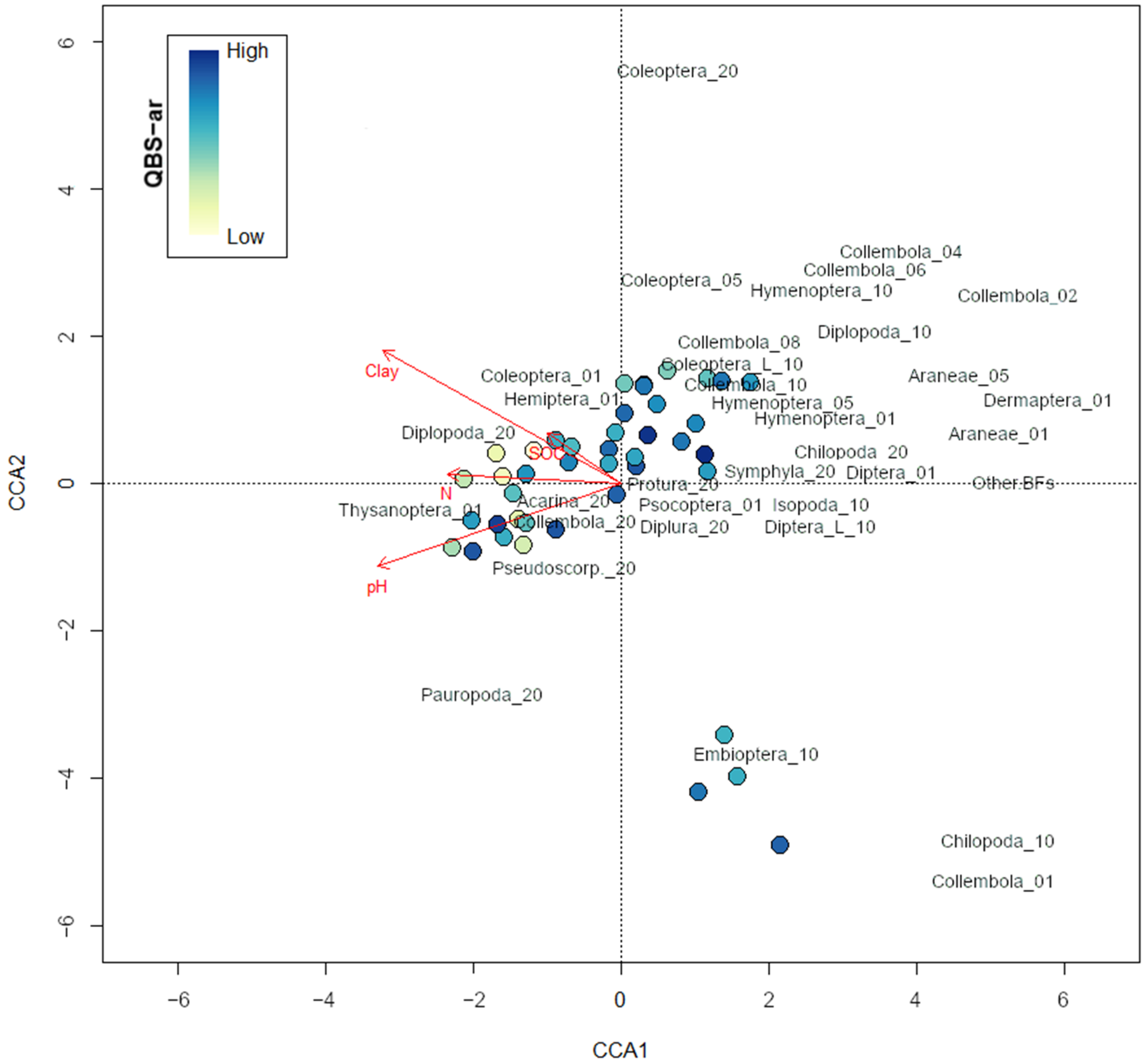
Effect of abiotic variables. Variance decomposition using CCA showed that 20.15% of the total variation in species composition (total scaled Χ² = 1.40) was constrained by the environmental variables considered in the model (clay content, N, pH, and SOC). The remaining 79.85% of the variation was unconstrained, reflecting factors not captured by the measured variables. The first canonical axis (CCA1) explained 45.38% of the constrained variation, while the second axis (CCA2) provided an additional 32.24%, thereby accounting for 77.62% of the explained variance. The environmental variables collectively have a measurable influence on species composition; however, a significant portion of the variation remains unexplained. Permutation tests indicated that clay content, N, and pH significantly contributed to the observed variation (p-value < 0.001), with pH explaining the largest proportion of variance (Χ² = 0.09, F = 3.11). Conversely, SOC did not show a significant effect (p-value = 0.85), suggesting that it does not substantially influence community distribution. The eigenvalues for the first two constrained axes (CCA1 = 0.13, CCA2 = 0.09) further highlight the importance of environmental gradients, with species distributions primarily structured along pH and clay content. The CCA biplot (Figure 2) visually underscores these relationships, showing distinct clustering of sites and species in response to these key environmental drivers. The distribution of QBS-ar values across the samples was explored in relation to the sites and environmental variables through the CCA biplot. Notably, the pH values indicated a negative relationship with QBS-ar: as pH increased, QBS-ar values tended to decrease, suggesting that higher pH levels may have a detrimental effect on soil biological quality, potentially reflecting a reduced biodiversity of soil fauna in more alkaline conditions. Similarly, clay content followed a comparable trend, with higher clay levels associated with lower QBS-ar values. This pattern implies that soils with a higher clay content may also exhibit reduced biological quality, possibly due to physical constraints on soil fauna mobility or decreased habitat availability in soils with reduced pore space and the number of air-filled pores.

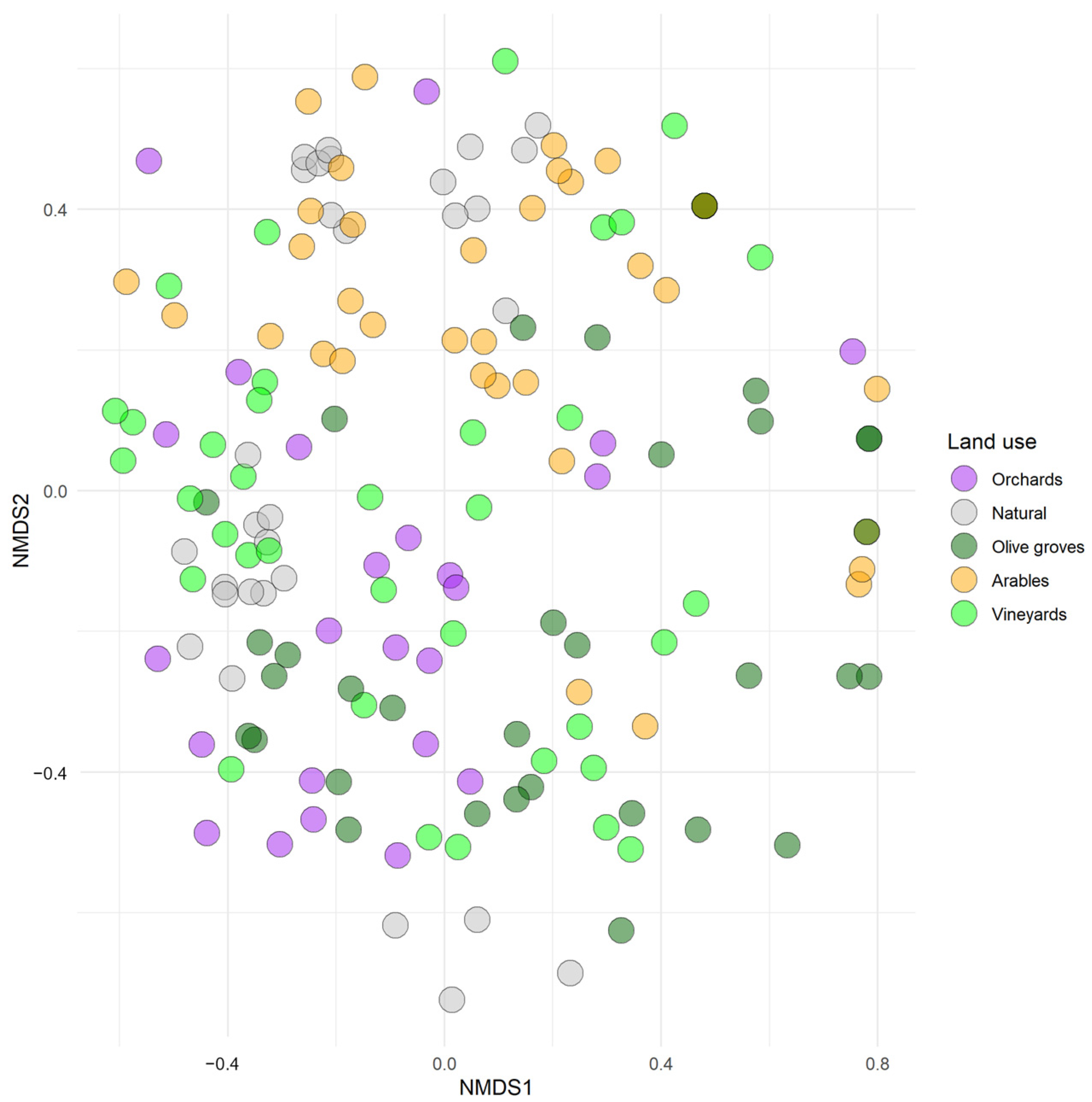
Community composition and similarity. Non-metric multidimensional scaling (NMDS, Figure 3) analysis was conducted in a two-dimensional space. The stress value was 0.30, indicating a relatively poor fit of the distances in the reduced space to the original data. However, the non-metric fit R² was 0.93, suggesting that the ordination preserved the rank-order relationships of the distances with high accuracy, successfully capturing 93% of the variation in the space. There is a certain degree of overlap between natural habitat subsamples and some agricultural habitats (Figure 3), such as in land used for arable crops and olive groves, which suggests that these types of land-use activities share some ecological features. In general, natural habitats appeared to be the least clustered group of observations due to a wider variability. Nonetheless, it can be observed that the arables represent a rather compact set of data. The ANOSIM (Jaccard distance, 9999 permutations, R = 0.24) confirmed the significant differentiation in terms of community composition between habitat types, as indicated by the highly significant p-value (0.0001). There is also a marked ecological separation between the different land-use patterns: crops like vineyards and olive groves showed some overlay, while other land-use practices like orchards and natural habitats are more closely distributed across the mean values. When agricultural soils, as a whole, were compared against natural habitats, they generally exhibited a wider range of dissimilarity values, which implies a higher internal ecological variability compared to soils supporting natural habitats. On the other hand, natural soil assemblages showed a lower range of dissimilarity linked to a more cohesive ecological structure compared to agricultural soils. In terms of observed biological forms, the analysis of shared species showed a high number of ubiquitous groups in the different land-use types. The lowest value is observed when comparing the communities of olive groves and arables (21) while orchards and olive groves share the highest number of taxa (31). For the remaining land-use categories, both the Soresen index, which measures similarity on the basis of shared species, assigning the double weight to common species, and the Jaccard index, which is similar to the previous one, but assigns less weight to shared species, returned rather high values of 0.9959 (95% C.I. 0.9599–1.0000) and 0.9796 (95% C.I. 0.8357–1.0000) respectively, indicating an almost identical composition among the communities. The Morisita–Horn index value (0.7892, with a 95% C.I. of 0.7542–0.8242) suggests that the communities of orchards and vineyards had a significant, though not complete, overlap. Conversely, the regional overlap index shows a higher value (0.9493, with a 95% C.I. of 0.9383–0.9603), indicating a greater degree of similarity between the communities. This second metric provides a broader measure of species overlap by considering all species regardless of their relative dominance. This higher value suggests that, while the relative abundances of dominant species differ, the overall species composition remains largely shared between the two communities. Generally speaking, the similarity values for both Morisita Horn and regional overlap estimated for each pair of land use indicate that natural soils exhibit a marked similarity when compared to other land uses, suggesting that agricultural soils, while similar, appear to be a subset of natural soils (Figure 4).

4. Discussion

The findings of this study are far from providing an exhaustive picture of the edaphic biodiversity of agroecosystems and the differences between these communities and those characteristic of natural and semi-natural environments. However, the results of this study provide some interesting insights into the ecological and biological characteristics of soil communities across different land uses. By analyzing a comprehensive set of samples from different land-use types, including some agricultural and natural habitats, it was possible to highlight some interesting patterns in biological forms, biodiversity indices and community composition. The QBS-ar index confirmed its sensitivity in measuring the differences in biodiversity between land uses that differ radically in history, land cover and management, as well as between soils with similar land uses [38]. Natural habitats consistently exhibited the highest QBS-ar values, reflecting their complex communities with high biodiversity values. Conversely, olive groves showed values closer to those of arable soils, highlighting a lower biological quality compared to other woody crops such as orchards. This similarity is supported not only by the Kruskal–Wallis test and the following post hoc comparisons but also from the results of the ANOSIM that revealed significant differences in term of biological forms composition among the various land-use types, with a notable separation between agricultural soils and natural habitats (R = 0.24). However, moderate R-values suggest similar ecological characteristics between agricultural soils supporting olive groves and arables. The general similarity across the communities of different agricultural soils could be attributable to shared environmental factors or similar management regimes. Within agricultural soils, however, it is possible to note that olive groves, despite being a woody crop, may share ecological characteristics with more intensively managed agricultural systems such as arables. This observation is probably linked to a generalized environmental stress rather than to common practices. While arables are characterized by being more intensively managed agricultural systems, olive groves are often cultivated, especially in the Mediterranean area, under “aridicultural” regimes and with reduced and more fragmented grass cover. The same decrease in QBS-ar and diversity values was also observed in vineyards that were routinely tillaged compared to those managed with ground cover vegetation [7].

The SIMPER analysis highlighted the taxonomic disparities driving these differences. Notably, arable soils exhibited the greatest taxonomic divergence compared to other land-use types, particularly orchards. Compared to vineyards and orchards, arables and olive groves differed in having a greater abundance of hemiedaphic and epigeic biological forms. This may reflect the ability of this more mobile component of the soil fauna to more easily recolonize soils affected by stressful conditions [39].

The SADs based approach proved to be very useful in providing critical insight into the diversity and complexity of soil communities. Communities following the Zipf–Mandelbrot distribution model, such as orchards, exhibited moderate slopes indicative of complex, stable systems with a limited number of dominant species, and a long tail of uncommon taxa. In contrast, arable soils were frequently associated with the Motomura niche pre-emption model; characterized by steep slopes reflecting low evenness, reduced biodiversity, and dominance by a few taxa. This result is consistent with what has also been observed in studies with greater taxonomic detail, which attest to the belief that habitats most influenced by human activity are characterized by a greater proportion of dominant species [40].

Despite the moderate quality of the representation offered by the CCA, it is quite clear that some community characteristics were explained by the environmental variables considered, with pH and clay content being the most significant factors. The negative correlation between pH and QBS-ar values suggests that alkaline soils may limit certain biological processes thus potentially reducing habitat suitability for certain taxa [41,42,43,44]. Similarly, higher clay content was associated with lower QBS-ar values, probably due to physical constraints on soil fauna mobility and habitat availability in more compact soils [45]. Conversely, unlike what has been reported in other studies [46,47], SOC did not significantly affect community composition.

The comparison between agricultural soils and natural habitats has not only highlighted the differences between these categories but also shed light on the relationships between two completely different categories of land use. In the reduced dimensionality space described by the non-metric MDS, the sub-replications relating to natural soils show a rather sparse distribution that is more often associated with other types of woody crops, as opposed to the tighter clustering of arable soil communities. However, this pattern is strongly supported by the ANOSIM run on the complete dataset showing that agricultural and natural habitats differ ecologically, with some transitional zones and shared ecological characteristics between certain groups. The strong similarity shown by the regional overlap index estimate between the habitat pairs, including those of the natural habitats, offers the possibility of a further comparison. Despite the same structure and similarity in terms of biodiversity values, arables and olive groves show a rather low coefficient, which probably indicates a different composition in terms of biological forms but having similar EMI scores. Nevertheless, similar values emerge from the comparison between arables and natural habitats, but characterized by markedly different complexity and richness. This comparison becomes more significant when the Morisita–Horn index is considered and whose lower values, compared to the regional overlap index, highlight a certain difference between the communities in terms of the relative distribution of dominant species. Agricultural soils appear to be subsets of the natural soils, as they share a large proportion of the biological forms as evidenced by the SIMPER analysis, but with a variation in their relative abundances of the dominant species. The diversity between agricultural and natural soils is subtle but ecologically relevant. This may draw attention to the fact that some agricultural practices or farm management systems (such as viticulture or fruit cultivation) may still feature some characteristics of natural edaphic communities, but with alterations in species structures and relative abundances.

The observed patterns have important implications for both land management and conservation strategies. The higher biological quality and diversity associated with natural habitats and certain woody crops, such as orchards, underscore the value of promoting alternative and less intensive agricultural practices and the preservation of natural areas to support and maintain soil biodiversity and ecosystem services [48].

5. Conclusions

Based on our study, the QBS index has been shown to be a very sensitive tool for measuring changes in communities in response to treatments applied to agricultural soils [13,47,49]. This index, together with related data on community composition and soil physicochemical characteristics, would seem to offer a more complete overview of soil biodiversity in different habitats.

The enormous complexity of the edaphic communities evidenced by previous studies [50] and revealed in this work once again highlights how the use of metrics not only of diversity but also of structure should be promoted, because they provide important information on the degree of community complexity. This complexity is directly linked to the stability of the environment and results not only from the breakdown of individual biological forms but also from the dynamic and numerical relationships between them. Furthermore, it is essential to extend harmonized and shared monitoring and data collection protocols so that we can enable the extension and improvement of the consistency of the results from region-wide surveys.

The results, although partial, that have emerged from this study are important considering the relevance of ecosystem services provided by edaphic communities [5,6,7,51], and emphasize the need to evaluate and promote an awareness amongst the farming community [52] of the importance of maintaining a healthy and robust soil biota in agricultural soils. Furthermore, these results confirm the importance, as already underlined by [46], of including the analysis of soil biodiversity in large-scale studies for a better understanding of the effects of global change on soil arthropod communities. The methods adopted in our work, as well as those recently suggested by [50] to evaluate the explanatory weight of environmental and agronomic covariates on selected bioindicators, could represent a basis for defining a global soil biota monitoring system.