Abstract
Catastrophic wildfires impacted large areas of western Kangaroo Island (KI), South Australia in 2019–2020, burning habitat for many species, including large proportions of the distributional range of the KI micro-trapdoor spider Moggridgea rainbowi, which led to it being listed as Endangered under Australia’s Environment Protection and Biodiversity Conservation Act (EPBC Act). In order to assess population genetic structure in M. rainbowi and detect diagnosable lineages and their distributional patterns across KI, 28 individuals were genotyped for 2495 loci, sampling from all known populations of the species. Population genetic and phylogenetic analyses of nuclear and mitochondrial sequence data provided strong support for three Evolutionarily Significant Units (ESUs) within M. rainbowi; two populations on eastern KI and a heavily fire-impacted western population. High levels of divergence and fixed allelic differences between 5 and 16% indicate a lack of gene flow between ESUs and long periods of isolation. Distributional patterns of these lineages match likely locations of isolation events caused by successive changes to sea level during the Quaternary (2.58 million years ago to present), which led to KI being intermittently connected to the mainland or separated into one or more islands. Our findings have strong conservation implications for M. rainbowi and highlight the importance of inclusion of population genetic structure to inform conservation strategies and to conserve lineage biodiversity at the species level and below.
Keywords:
Moggridgea; trapdoor spider; island endemic; Kangaroo Island; molecular genetics; RAD-seq; fire 1. Introduction
Trapdoor spiders of the family Migidae are small to medium-sized spiders, which construct and occupy short trapdoor burrows in tree trunks, or in the ground [1,2]. The family has a typical Gondwanan distribution, being found in all southern continents except India [3]. In Australia, the family is represented by four genera: the Australian endemic Bertmainius Harvey, Main, Rix and Cooper, 2015, and Heteromigas Hogg, 1902, and the more widespread genera Migas L. Koch, 1873, and Moggridgea O. Pickard-Cambridge 1875, which occur on more than one continent. Migid species typically have high habitat specificity and disjunct and restricted distribution patterns with frequent short-range endemism [4,5], resulting in elevated conservation risk [6,7] and leading to several species internationally being identified as of conservation concern [2,8,9]. Studies have revealed strong genetic structuring at the population level for Calathotarsus Simon, 1903 in Argentina [4] and Bertmainius in Australia, likely as a result of low vagility and a typically sedentary nature, and revealed for both genera cryptic speciation amongst geographically close species with discrete, highly localized distributions [2,10].
The genus Moggridgea is recorded from South Africa and southern Australia [3,11,12] and has an enigmatic history. Molecular dating indicates the only known Australian species, Moggridgea rainbowi (Pulleine, 1919), diverged from its nearest congeners in South Africa between 2.27 and 16.02 million years ago (MYA), post-dating separation of Africa from Gondwana and pre-dating human mediated dispersal. These analyses supported a hypothesis of colonization via trans-oceanic dispersal, the first documented case for a mygalomorph spider [13].
Moggridgea rainbowi occurs on Kangaroo Island (KI), an island with an area of 4405 km2, situated around 15 km off the south coast of South Australia (Figure 1a). The species has a predominantly coastal distribution on KI and is found in scattered populations in creeklines, stretching from the northwest of the island to the northeast [9]. Individuals occupy shallow trap door burrows, ca. 7 cm deep, which are constructed in the banks of small, low energy creeklines [9]. KI has a Mediterranean climate, with dry hot summers and cooler, wetter winters; around a third of the annual rainfall occurs during the winter months (between May and September), and rainfall varies markedly between the east of the island (ca. 450 mm) and the west (ca. 1000 mm) [14]. About a quarter of KI is designated for conservation, as Wilderness Protection Areas (WPA), Conservation Parks (CP), and National Parks, most of which are located in western KI [14]. During December 2019 and January 2020, catastrophic wildfires impacted western KI, burning nearly half of the island, much at high severity, including nearly all conservation reserves to the west of the island [9,15]. Most of the known western populations of M. rainbowi were impacted by fire, with surviving individuals known only from small, isolated patches of unburnt refugia [9]. This, in combination with threats to the species posed by land clearance, incursion by Bridal Creeper, Asparagus asparagoides (a ground-matting weed of national significance [16]), changes to hydrology, climate change, drought, and the threat of future fire, both wild and human-mediated, led to the species being listed as Endangered under Australia’s Environment Protection and Biodiversity Conservation Act (EPBC Act) in 2022 [17]. Detailed surveys conducted following the 2019–2020 wildfires on KI have better delineated the distribution of the species and located additional populations [9].
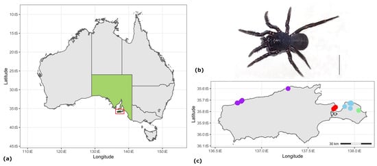
Figure 1.
(a) Map of Australia, with South Australia shown in light green and Kangaroo Island highlighted by a red box; (b) male M. rainbowi from Shorty Road, Chapman River, scale = 5 mm; (c) map of Kangaroo Island showing collection locations for M. rainbowi, with sample areas depicted as coloured circles; east: Pen: Penneshaw (Baudin CP and Penneshaw) in blue; Chapman River (CR) in green; American River (AR) in red; and West: (Cape Forbin, Cape Cassini and Cape Torrens WPA) in purple.
Harrison et al. [11,13] uncovered phylogeographic structuring in M. rainbowi, with monophyletic groups of mitochondrial haplotypes representing the two sub-populations known at the time of the study (American River and Western River, west KI). High population structuring within a species is indicative of geographical or reproductive isolation and, as such, is relevant to the conservation status of the species, as well as the development of strategies for conservation management (e.g., via translocations [18]). Such diverged populations may represent evolutionarily significant units (ESUs) [19]. Whilst the definition of ESUs has been the subject of debate (for example, [20,21]), here we adopt a definition, as proposed by Fraser and Bernatchez [22], of an ESU as a lineage that demonstrates highly restricted gene flow from other lineages within the species. We also consider the additional Moritz criterion [23], which proposes that ESUs should show reciprocal monophyly in phylogenetic analyses of mitochondrial DNA sequence data. Whilst species remain the standard unit used in conservation assessments, the use of other measures of biodiversity, such as phylogenetic diversity [24] or ESUs [23], may provide alternative approaches that escape the limitations of a reliance on taxonomic species delineation [25]. By doing so, they may provide important information for protecting biodiversity and enhancing genetic diversity at or below the species level, to inform subsequent conservation planning [26,27,28,29]. This becomes particularly relevant at a regional scale in relation to large-scale threat events that differentially impact ESUs, such as the 2019–2020 wildfires, which impacted western populations of M. rainbowi.
Here, we use molecular techniques, including mitochondrial DNA sequencing and reduced representation population genomic analyses, to examine the population structure of the threatened M. rainbowi on KI. We find a strong phylogenetic structuring in populations of M. rainbowi, with analyses delineating three ESUs, indicative of patterns of profound isolation and highly restricted gene transfer between sub-populations. We discuss this in relation to threats posed to each of the ESUs and how this relates to the conservation of the species. We propose this as a case study to illustrate the importance of population structural analyses in conservation planning for threatened species.
2. Materials and Methods
Thirty-four tissue samples were available from M. rainbowi for molecular genetic analysis, collected between 2013 and 2022 from Kangaroo Island (KI), South Australia (Figure 1, Table 1). Specimens were extracted from burrows, and transferred to 100% ethanol. Where possible, a leg was removed and the spider released, which was the case for 2 of the 34 samples. Most of the samples were collected between 2 September 2019 and 6 April 2022 under permit number U26935 from the South Australian Department of Environment and Water. The species was not listed as threatened at the time these samples were collected; however, due to the potential threatened status of M. rainbowi, extensive sampling at each collection locality was not deemed possible, and so we needed to supplement our collections with samples from a study conducted 10 years ago by Harrison et al. [13]. Female migids are known to be long-lived and to stay in a single burrow throughout their life [7,30] and therefore population structure analyses are unlikely to be strongly influenced by the temporal difference in collections. These 2013 samples were DNA extracts from American River (SAMA numbers, Table 1), used to reconstruct the phylogeny of the genus Moggridgea [11,13].

Table 1.
Sample information for M. rainbowi. Institution code: South Australian Museum, Adelaide (SAMA); Reg Number—Registration number of voucher specimens; CP: Conservation Park; WPA: Wilderness Protection Area.
Location and voucher information for the samples are presented in Table 1. The samples can be grouped into four different regions, as shown in Figure 1c: 13 samples were from Baudin CP and Penneshaw (Pen); 5 from Chapman River (CR); 10 from American River (AR) (east); and 6 from Cape Forbin, Cape Cassini and North (N.) Cape Torrens WPA (West). Vouchers are deposited at the South Australian Museum, Adelaide.
Genomic DNA was extracted from a single leg using the MagMax CORE kit on a KingFisher Duo Prime purification system (Thermo Fisher Scientific, Scoresby, VIC, Australia), according to the manufacturer’s protocol for fresh tissues. The amount of DNA was quantitated on a fluorometer using QuantiFluor dye (Promega, Madison, WI, USA). The samples were normalized to 1 ng/µL for subsequent DNA sequencing. A reduced representation of the genome of each sample was prepared for sequencing [31]: double-digest restriction site-associated DNA sequencing (RAD seq), with duplicate reactions included in the analysis as technical replicates. Following the protocol of Poland et al. (2012) [32], the samples were double-digested using restriction enzymes PstI-HF and HpaII (NEB BioLabs, Ipswich, MA, USA); then, the cut sites were ligated with different-length indexed sequencing adapters. To determine the appropriate amount of adapter required (1 µL), an adapter titration test was performed on a single-digested DNA extract, prior to adapter ligation for the rest of the samples. Once each sample was uniquely indexed, they were pooled and PCR-amplified with Illumina sequencing primers, AATGATACGGCGACCACCGAGATCTACACTCTTTCCCTACACGACGCTCTTCCGATCT (Forward) and CAAGCAGAAGACGGCATACGAGATCGGTCTCGGCATTCCTGCTGAA (Reverse). Final fragment length distribution and molarity of the RAD seq library was determined on a TapeStation 2200 using high-sensitivity ScreenTape and reagents (Agilent Technologies, Santa Clara, CA, USA). Sequencing was conducted on a NovaSeq 6000 SP single lane at the Australian Genomic Research Facility (AGRF) in Melbourne with 100 bp single-end read cycles.
The generated sequences were processed with Stacks 2 (ver. 2.6.1, see https://catchenlab.life.illinois.edu/stacks/, accessed on 7 May 2023) using the de novo analysis pipeline developed to call loci from restriction-digested, short-read sequences, where there is no available reference genome [33]. The FASTQ file was quality-checked with FastQC (ver. 0.11.8, see http://www.bioinformatics.babraham.ac.uk/projects/fastqc/, accessed on 7 May 2023). Raw data were cleaned and de-multiplexed into individual samples with the process_radtags command in Stacks. All reads with uncalled bases and/or low-quality scores were removed, the presence of the restriction enzyme cut site was checked, and the reads were trimmed to 75 bp to remove low quality ends identified in the FASTQC analysis. The per-sample raw read count distribution was obtained from the log files using the stacks-dist-extract command and summary plots were produced in the R software (ver. 4.2.1, R Foundation for Statistical Computing, Vienna, Austria, see https://www.R-project.org/, accessed on 7 May 2023). Sequences were aligned with loci for each individual (-M number of mismatches allowed = 3) and then matched to a catalogue of all loci (-n number of mismatches allowed between loci of individuals and the catalog = 3) using denovo_map.pl. in Stacks. The populations script from Stacks was run on the output of the de novo assembly, keeping only single-nucleotide polymorphisms (SNPs) where the minor allele was observed at least three times in the metapopulation, that were present in all four localities and in 90% of all samples, then exporting a single SNP per locus for all the samples in variant call file (vcf) format. Genotype coverage per sample was obtained from the log file gstacks.log.distribs and samples with an average locus coverage of ≥10 reads were kept for further SNP filtering and population genetic analyses in the R software. Duplicates were compared to calculate error rates in the SNP calling (13 out of 34 samples passed the coverage filter of average locus coverage of ≥10 reads for both) and the replicate with the best coverage was kept for further analyses for 32 samples (SAMA28346.1 and jm0107B did not pass the ≥ 10 reads average coverage filter). GenBank accession numbers are presented in Table S1.
The SNP data and associated location information were read into a genlight object (Ref. [34]; adegenet R package) to enable processing with dartR (ver. 2.0.4., [35]; see https://www.rdocumentation.org/packages/dartR/versions/2.0.4, accessed on 7 May 2023). Missing data per sample were visualized using the gl.smearplot function and four individuals with a large amount of missing data (>70%) were removed. Further filtering was undertaken using gl.filter.callrate to remove any loci that were now monomorphic and to provide a final dataset with a call rate of 100% (no missing data, threshold = 1.0). Low sample sizes (n = 5 and 6 for CR and west) precluded any further filtering for departures from Hardy–Weinberg equilibrium or linkage disequilibrium.
For analysis of the SNP data, we first used the principal coordinates analysis (PCoA) ordination to identify genetic clusters based on a Euclidean distance matrix (gl.pcoa and gl.pcoa.plot functions of dartR). A further investigation of genetic structuring was carried out via a Discriminant Analysis of Principle Components (DAPC), implementing the function dapc from the adegenet R package [36]. The number of clusters in the data was first inferred using k-means clustering of principle components (find.clusters), with the optimal number chosen based on the lowest associated Bayesian Information Criterion (BIC). Then, the DAPC was run using the clusters defined by k-means as a prior. The data were transformed via Principle Component Analysis (PCA), the number of principle components to be retained were chosen, and then a Discriminant Analysis (DA) carried out, which maximizes the separation between groups while minimizing variation within groups. Each sample could then be assigned into a cluster and population assignment before and after the DAPC was examined. For comparison with the analyses based on principle components, the Bayesian clustering approach using STRUCTURE (Ref. [37], ver. 2.3.4, see https://web.stanford.edu/group/pritchardlab/structure_software/release_versions/v2.3.4/html/structure.html, accessed on 7 May 2023) was implemented in R (gl.run.structure from the dartR package). The admixture ancestry model with correlated allele frequencies was run to determine the optimal number of genetic clusters and to assign individuals to groups. We used prior locality information to assess values of K from 1 to 8, and performed three independent runs with results based on a Markov Chain Monte Carlo (MCMC) of 1,000,000 steps, of which the first 10,000 were discarded as burn-in. The optimal value of K was determined using the change in the second order of likelihood, ΔK method (Ref. [38]; gl.evanno) and each individual’s estimated membership coefficients for each cluster were then plotted (gl.plot.structure). The eastern KI samples were subset from the original genlight object (gl.keep.pop) and filtered to remove loci that were now monomorphic. A separate STRUCTURE run was carried out on these samples as above.
We determined the amount of fixed allelic differences in loci between the clusters identified in the population genetic structure analyses presented above (gl.fixed.diff function in dartR). Testing was for absolute fixed differences between populations, and p values were calculated for the observed fixed differences by simulation (significance level, alpha = 0.05). The results of the fixed difference analysis between populations were visualized as a heatmap (gl.plot.heatmap).
The neighbor-joining method for reconstructing phylogenetic trees (Ref. [39]; Nei’s genetic distance matrix) was carried out on the SNP dataset in the R package Ape. A Maximum Likelihood (ML) analysis of the SNPs was undertaken in IQ-tree (ver. 1.6.12; see http://www.iqtree.org/, accessed on 7 May 2023, [40]), using the ultrafast bootstrap method (5000 pseudo-replicates, [41]) and the GTR [42] model of evolution with ascertainment bias correction (+ASC) to account for the lack of constant sites in the alignment [43].
For sequence analyses, a partial fragment of the mitochondrial cytochrome c oxidase subunit 1 (COI), and the ribosomal Internal Transcribed Spacer gene (ITS rRNA-including ITS1, 5.8S rRNA, ITS2), were PCR-amplified for all the samples collected post 2019 to add to the five samples from American River obtained from the 2013 dataset [13]. Primers used were the universal COI primers LCO1490 (5′-GGTCAACAAATCATAAAGATATTG-3′) and HC02198 (3′-TAAACTTCAGGGTGACCAAAAAATCA-5′) [44], and ITS primers G923 (5′-CGTAACAAGGTTTCCGTAGGTGA-3′) and G925 (5′AGAGAACTCGCGAATTCCACGG-3′) [10]. COI PCRs were carried out in a 25 µL reaction volume consisting of nuclease-free water, 1 X Immolase PCR buffer, 1.5 mM MgCl2, 0.8 mM dNTP mix, 0.05 mg/mL BSA, 0.24 µM primer, 0.5 u Immolase DNA polymerase (Bioline; NSW, Australia) and approximately 0.5–2 ng of extracted DNA. The cycling conditions for COI were; 95 °C for 5 min, (95 °C for 45 s/48 °C annealing for 45 s/72 °C for 60 s) × 39 cycles, with a final extension at 72 °C for 10 min. Due to the presence of multiple products in the COI amplicons, the PCRs were repeated with short species-specific primers designed in Geneious (ver. 10.4.1; see https://www.geneious.com, accessed on 7 May 2023), 5′-CTTCATTAGTAGATGTAGGAGTGGG-3′ (M1764) and 5′-CCTCCTGCAGGGTCAAAAA-3′ (M1765) as above, but with an annealing temperature of 50 °C. ITS PCR conditions were 94 °C 9 min, (94 °C 45 s, 68 °C 45 s, 72 °C for 60 s) × 6 cycles with 1 °C negative increments (94 °C 45 s, 62 °C 45 s, 72 °C for 60 s) × 35 cycles, 72 °C for 10 min using the enzyme Amplitaq Gold (ThermoFisher Scientific). Product purification and Big Dye Terminator sequencing were carried out at AGRF Adelaide. The resulting sequence files were aligned in Geneious to produce a 287 bp COI and a 683 bp ITS alignment. GenBank accession numbers for all sequences are presented in Table S1. Maximum likelihood trees based on the COI and ITS alignments were generated in Geneious using RAxML (ver. 8.2.11, see https://github.com/stamatak/standard-RAxML, accessed on 7 May 2023; [45]) with rapid bootstrapping and the best-scoring tree was searched for under the GTR + G model of evolution [46], with 1000 bootstrap replicates. Phylogenetic trees were visualised in the R software (ggtree package [47]) and trees were rooted on the western clade to aid the comparison between COI and ITS.
3. Results
3.1. SNP Data
The Moggridgea rainbowi RAD-seq dataset consisted of 539,976,913 reads (55 Gb of data). After cleaning in Stacks, 5.5% were trimmed for adapter sequence; 0.1% of reads had no barcode and were removed; 0.1% were low quality and were removed; and 0.8% were dropped as the RAD cutsite was not found. This left 496,192,005 cleaned reads (91.9% of the raw data), which were de-muliplexed into individual samples. The number of reads per sample varied considerably over the dataset, from 25,872 to 23,702,407, with a mean of 6,361,436 reads per sample, potentially reflecting variability in the quality of the samples. However, there was no evidence for the different locations having major differences in sequencing success per sample, other than the region with the most samples (Pen) having a lower average number of reads (Figure S1a). The proportion of reads remaining after cleaning was plotted for each sample and most samples retained over 80% of their reads (Figure S1b). Three replicates were removed from further analyses, as they had less than 20% reads remaining after the process_radtags step (Figure S1b). All three samples had a duplicate sample remaining for the SNP calling.
Thirteen duplicate samples, which were technical replicates and had an average read coverage of ≥10 reads, were compared for SNP calls, with genotyping error rates measured as the proportion of SNP mismatches between replicate pairs. For the 26 samples, 81,856 binary SNPs were output from Stacks with 1.33% missing data. Further filtering in dartR to leave no missing data retained 53,612 SNPs for comparing error rates. Genotyping error rate ranged from 0.3% to 1.4%, with an average of 0.6%. A Neighbour-Joining tree of these samples showed each duplicate grouping together, giving confidence in the SNP calling parameters (M = 3, n = 3) used in the Stacks pipeline (Figure S2).
The best coverage samples from each replicate gave 25,999 binary SNPs when called in Stacks (5.31% missing data); however, four samples were removed after an examination of the amount of missing data in dartR smearplots (jm0099, jm0107C_2, jm0107D, jm0107E_2; all from Penneshaw; Figure S3). The final data matrix consisted of 28 individuals genotyped for 2495 loci and had no missing data (eight samples from Baudin CP and Penneshaw (Pen); five from Chapman River (CR); six from Cape Forbin, Cape Cassini and Cape Torrens WPA (west); and nine from American River (AR)).
3.2. Population Genetic Clustering
In the PCoA analysis (Figure 2), three major clusters were found that correspond to samples from the west of the island, samples from the American River, and samples from Baudin CP, Penneshaw and the Chapman River clustering together (Pen and CR). The single sample from Cape Cassini (purple) is separated from the other western samples by PCA Axis 1, which explains 44.5% of the variation in the data, and clearly separates the western and eastern sides of the island, matching to longitude as illustrated on the map insert. The second PCA Axis explains a further 23.7% of the variation, and separates the American River samples from the other eastern KI samples.
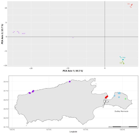
Figure 2.
Principle coordinates analysis (PCoA) with Moggridgea rainbowi samples coloured by location; east: Pen (Baudin CP and Penneshaw) in blue; CR (Chapman River) in green; and AR (American River) in red; west: (Cape Forbin, Cape Cassini and Cape Torrens WPA) in purple. Dashed line on map insert indicates the approximate location of the isthmus between the Dudley Peninsula and the rest of KI.
Discriminate Analysis of Principle Components (DAPC) additionally returned three clusters based on two linear discriminants, and the sequential k-means clustering also estimated three distinct clusters as a prior for the DAPC (Figure S4). These clusters represent the same groupings as the PCoA; Cluster 1 contains the samples from Baudin CP, Penneshaw and Chapman River; Cluster 2 has the American River samples and Cluster 3 contains the samples from west.
Analyses with STRUCTURE unambiguously chose three populations in the data (Figure 3a,b). Plots of assignment to K = 3 (Figure 3b) showed the single sample from Cape Cassini (jm0115, west) as admixed between the western and two eastern populations; however, it may also be representative of a distinct population. Chapman River and Penneshaw/Baudin CP samples clustered together in a single population, American River samples remained distinct, and Cape Torrens WPA and Cape Forbin samples formed the western cluster (Figure 3b).
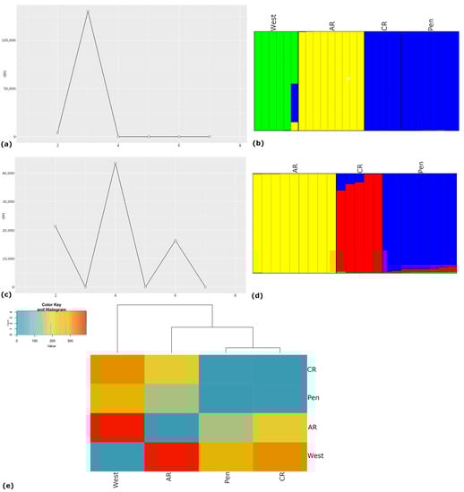
Figure 3.
(a) STRUCTURE clustering of the M. rainbowi samples; plot of the change in the second order of likelihood, ΔK from the STRUCTURE results for each value of K (horizontal axis); (b) results of the STRUCTURE analysis for K = 3; east: Pen (Baudin CP and Penneshaw); CR (Chapman River); and AR (American River); west: Cape Forbin, Cape Cassini and Cape Torrens WPA. Each column represents a single individual’s estimated membership coefficients for each cluster; (c) STRUCTURE clustering of the eastern Kangaroo Island Moggridgea rainbowi samples; plot of the change in the second order of likelihood, ΔK from the STRUCTURE results; (d) results of the STRUCTURE analysis for K = 4; Pen (Baudin CP and Penneshaw); CR (Chapman River); and AR (American River). Each column represents a single individual’s estimated membership coefficients for each cluster. Colors represent distinct populations; (e) heatmap of allelic fixed differences between Moggridgea rainbowi populations: Chapman River/Penneshaw/Baudin CP (CR/Pen), American River (AR), and west; with IQ tree from the SNP data. Colors in the pairwise population comparisons reflect the number of fixed allelic differences among the populations based on the color key in the top left hand corner.
Further hierarchical analyses examining the eastern KI samples as a separate group (22 genotypes, 1475 polymorphic SNPs) identified four populations as the level of genetic sub-structuring (Figure 3c). However, the STRUCTURE plot showed only three major clusters (Figure 3d). American River samples were distinct and Chapman River samples showed evidence of admixture with genetic material from Penneshaw/Baudin CP (Figure 3d). The gene flow appears to be largely from Penneshaw/Baudin CP into the Chapman River population (Figure 3d). The fourth population, shown in light green, was a very minor component of individuals from Chapman River/Penneshaw/Baudin CP and one individual from American River, and possibly represents a population that has not yet been sampled in our study (Figure 3d).
3.3. Fixed Allelic Difference Analysis
All the population genetic structure analyses pointed to three distinct populations in the data: west; American River; and Penneshaw/Baudin CP /Chapman River, all located on the Dudley Peninsula (Figure 2). The presence of fixed allelic differences was examined between these three groupings, which occurs when one population is homozygous for allele 1 and the second population is homozygous for an alternate allele, as there were no missing data in the final dataset. There were 16% fixed differences between the west and American River; 10% fixed differences between the west and Penneshaw/Baudin CP/Chapman River; and 5% fixed differences between Penneshaw/Baudin CP/Chapman River and American River (Figure 3e). All comparisons were significantly different by simulation, which estimated the expected false-positive rate in pairwise comparisons (p < 0.001). If Penneshaw/Baudin CP and Chapman River samples were separated and compared, no fixed allelic differences were found, suggesting that gene flow likely occurred between these two localities.
3.4. Phylogenetic Analyses of COI and ITS Sequences
Sequencing a short species-specific fragment of COI enabled a COI dataset (assumption maternally inherited, non-recombining) to be produced for contrast with the bi-parentally inherited nuclear data for representatives from all localities except Cape Forbin (west), where the sequences were still from multiple mitochondrial PCR products. Maximimum Likelihood analyses of the COI and ITS sequences gave differing phylogenetic trees (Figure 4a and Figure S5). The COI (287 bp) tree showed recriprocal monophyly for the four different regions, although bootstrap support for the groups was low (Figure 4a). The ITS tree showed separate eastern and western monophyletic groups (BS support 100%), with the exception of the sample from Cape Cassini (jm0115), which showed a distinct ITS haplotype that grouped with the eastern samples (Figure S5). A common ITS haplotype was also found in several individuals from each of the three eastern locations.
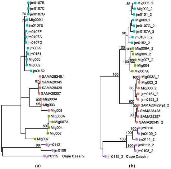
Figure 4.
Comparison of phylogenetic trees. (a) Maximum likelihood tree from the mitochondrial cytochrome c oxidase subunit 1 (COI) sequence dataset. Bootstrap proportions (>75%) for each node are shown. (b) Maximum likelihood tree topology from the SNP dataset generated in IQ-tree. Ultrafast Bootstrap proportions (>75%) for each node are shown. Sampling locations depicted as coloured circles at the tips are east: Pen (Baudin CP and Penneshaw) in blue; CR (Chapman River) in green; and AR (American River) in red; west: (Cape Forbin, Cape Cassini and Cape Torrens WPA) in purple. Cape Cassini sample is labelled in bold.
Phylogenetic analysis of the SNP dataset grouped the samples according to the four regions, giving a similar tree topology to the mitochondrial analysis with better support values, except for the position of the Cape Cassini sample (Figures S5 and S6).
4. Discussion
In this study, we provided evidence of strong population genetic structuring for the endangered KI micro-trapdoor spider, M. rainbowi and delineated the distribution of ESUs across KI. We found strong support from analyses of both nuclear and mitochondrial markers for three distinct ESUs for M. rainbowi under genetic criteria proposed by Fraser and Bernatchez [21] and Moritz [23]. The ESUs occurred at American River, the Dudley Peninsula (both situated on eastern KI and separated by around 15 km, measured as a direct line), and western KI. The single sample from Cape Cassini, which is located in the mid-north of the island, ca. halfway between the western and the eastern populations, showed genetic differentiation from both the western KI population and the eastern populations, with Maximum Likelihood analyses of COI and SNP data grouping the Cape Cassini sample with the western population (Figure 4). However, further research involving more samples is needed to determine whether Cape Cassini represents an additional ESU.
In addition to the population differentiation, the presence of fixed allelic differences between American River and Dudley Peninsula, between American River and Western KI, and between Dudley Peninsula and Western KI populations indicate a level of genetic isolation, most likely resulting from the long-standing geographic isolation between these populations. We also cannot rule out the possibility that the populations are reproductively isolated, although there is evidence of an ITS haplotype being shared by the two eastern populations, which is likely a result of the incomplete lineage sorting for this marker. Moggridgea rainbowi diverged from its closest known congener in South Africa, and likely arrived on KI between 2.72 and 16.02 MYA [13]. It was possibly more widespread in the region during wet periods on the Australian continent, such as in the early Pliocene, and populations may have subsequently been restricted to wet creek systems following the aridification of the Australian continent during the late Pliocene and Pleistocene [48,49]. Sea-level changes in the Quaternary (2.58 MYA to present) resulted in KI intermittently being a part of the mainland during low sea stands in glacial periods, with the most recent glacial maximum low stand occurring around 20,000 years ago [50,51]. KI currently occurs as a single island and during high sea stands in interglacial periods [52] it has also existed as two or more islands, with a potential point of separation being the isthmus connecting the Dudley Peninsula with the rest of the island [53,54] (approximate location illustrated in Figure 2). It is plausible that isolation events occurred during periods when the Dudley Peninsula was divided from the rest of KI, separating this population from the remainder of the island and the combination of low vagility and a typically sedentary nature restricted gene flow during times that KI existed as one island. Separation among populations in this region of KI is also evident in the grasshopper Vandiemenella viatica (Erichson, 1842), which has chromosomally and genetically distinct populations in the Dudley Peninsula and American River regions, respectively, with a hybrid zone at the boundary of the two regions that led to restricted gene flow [55,56,57].
Our findings of isolated populations with a lack of gene flow between them, plus strong population structuring, indicates that the dispersal of individuals is highly restricted, matching what is known of other migid species in Australia and internationally [2,8]. The high population structure for M. rainbowi supports the findings of Harrison et al. [13] and is consistent with patterns detected in other migid genera, where population structure was shown to be a result of cryptic species occupying geographically close, discrete, and highly localized distributions [2,4,10]. For example, several species in the genus Bertmainius are highly endemic within wet creek systems near the summit of mountains in the Stirling Range in Western Australia, separated by dry valleys that restrict gene flow [2,10]. Such populations are likely to be at high risk from stochastic or anthropogenic local extinction events and there is substantial risk that post-threat recolonization or population recovery is slower than the extirpation rate [58]. The interpretation of conservation risk and subsequent conservation management strategies can vary depending on the level of biodiversity under consideration. For example, strategies to protect biodiversity may be different when targeted at the species level, rather than at the genetic level. This becomes especially important in the face of regional large-scale threat events, such as the 2019–2020 fires, where disjunct populations may face distinct conservation challenges, requiring a tailored approach to developing conservation strategies. In M. rainbowi, much of the distributional extent of the western ESU was impacted by a high-severity fire in 2019–2020, causing substantial population declines, and the ESU is now facing an imperiled future [9]. The American River and Dudley Peninsula ESUs, whilst not fire-impacted, face ongoing threats, including land clearance, the erosion of creek banks, changes in hydrology, fire, climate change, and invasion of the exotic ground clumping Weed of National Significance Bridal Creeper, Asparagus asparagoides [17]. Management of the individual populations needs to be tailored accordingly and, as such, the findings from this study raise important conservation considerations for M. rainbowi in relation to the resilience of the ESUs to threats, their ability to recover, and the conservation strategies needed to protect them.
The accurate delineation of species or ESUs is critical for assessments of biodiversity and subsequent conservation planning [26,27,28]; however, whether the ESUs identified in this study represent one or more separate species, or whether they are a result of structuring within M. rainbowi, requires further research. Currently, males are only known from the American River ESU, and an integrative approach, combining a detailed analysis of male morphology from each of the ESUs, plus ecological and molecular data, is required to determine the taxonomic status of the populations. This case study illustrates how the utilization of population genetic data allows for the identification of conservation-significant biodiversity units, irrespective of taxonomic status. Taxonomy plays a vital role in the delineation of species and their distribution [59,60]; however, two thirds of Australia’s estimated 320,000 invertebrate species are undescribed [61], and the taxonomic impediments, (the ‘Linnean shortfall’) caused by the large number of undescribed species and a limited workforce [62,63] mean that taxonomic revisions can take substantial time. While not replacing taxonomy, the evaluation of the genetic population structure of taxa that are likely at risk (for example, short-range endemic taxa and those substantially impacted by threat events) provides a mechanism for the rapid assessment of conservation risk for biodiversity units that otherwise could not be assessed.
The use of an integrative approach to conservation planning, which includes the consideration of population structure, is important to identify and preserve biodiversity across multiple levels (gene, population, species) [29] and to tailor conservation planning to the needs of distinct structural units. The occurrence of large-scale threat events, such as the 2019–2020 Australian wildfires, plus predictions of increasing severity and frequency of events due to climate change [64,65,66], highlights the need for a deeper consideration of population genetic structure in the development of conservation strategies in order to prevent an irreversible loss of genetic diversity. We demonstrate the application of population genomic data to reveal cryptic diversity within a threatened species of spider, identify relevant conservation units and inform conservation management.
Supplementary Materials
The following supporting information can be downloaded at: https://www.mdpi.com/article/10.3390/d15070827/s1. Table S1. Genbank accession numbers for Moggridgea rainbowi sequences and RAD-seq tags (SNP). Mitochondrial cytochrome c oxidase subunit 1 (COI); ribosomal Internal Transcribed Spacer gene (ITS). Figure S1. Number of reads per sample after cleaning in Stacks: (a) Spread of number of retained reads coloured by location; east: Pen (Baudin Conservation Park and Penneshaw) in blue; CR (Chapman River) in green; and AR (American River) in red; west: (Cape Forbin, Cape Cassini and Cape Torrens Wilderness Protection Area) in purple. (b) Proportion of retained reads for each sample. The mean value for all the samples is shown as a red dotted line. Figure S2. Unrooted Neighbour Joining tree of SNP data from the duplicate Moggridgea rainbowi samples that passed the read coverage filter. Coloured circles at the tips represent sample location: West (Cape Forbin, Cape Torrens Wilderness Protection Area) in purple, American River in red; Pen (Baudin Conservation Park and Penneshaw) in blue; and Chapman River in green. The number 2 after the sample name denotes the duplicate. Figure S3. Smearplot of the genotypes of the Moggridgea rainbowi samples coded as 0 (homozygous reference state 1), 1 (heterozygous) and 2 (homozygous for the alternate state). Missing data are coloured white. Figure S4. Discriminate Analysis of Principle Components (DAPC) for Moggridgea rainbowi samples (a) Value of Bayesian Information Criterion (BIC) vs number of clusters from the k-means clustering; (b) Plot of population membership before and after DAPC; colors represent membership probabilities (red = 1, white = 0) and blue crosses represent the prior cluster. Figure S5. Maximum likelihood tree from the ribosomal Internal Transcribed Spacer gene (ITS) sequence dataset. Bootstrap proportions (>75%) for each node are shown. Figure S6. Unrooted Neighbour Joining tree of the Moggridgea rainbowi SNP dataset. Coloured circles at the tips represent sample location; West (Cape Forbin, Cape Torrens Wilderness Protection Area, Cape Cassini) in purple, American River in red; Pen (Baudin Conservation Park and Penneshaw) in blue; and Chapman River in green.
Author Contributions
All the authors contributed to the project conceptualization. J.R.M. contributed collections, funding acquisition, supervision and writing the original draft and review and editing. T.M.B. carried out all genetic data generation, population and phylogenetic analyses, writing of the original draft, review and editing. S.J.B.C. contributed to funding acquisition, supervision and review and editing of the manuscript. All authors have read and agreed to the published version of the manuscript.
Funding
This research was funded in part by the Australian Federal Government’s Bushfire recovery Scheme, project number BWHR-T2_GA-2000663, by the South Australian state government’s Landcare led bushfire recovery grant scheme, number LLBRG210201, and by the Kangaroo Island Landscape Board, South Australia.
Institutional Review Board Statement
Not applicable.
Data Availability Statement
The RAD sequence data are deposited in the GenBank SRA (BioProject accession PRJNA961912). The analysed data and R codes are available on figshare; genotype matrix, https://doi.org/10.25909/23264948.v1, accessed on 7 May 2023; IQ-tree SNP analysis, https://doi.org/10.25909/23264957.v1, accessed on 7 May 2023; Rcode and input files, https://doi.org/10.25909/23264930.v1, accessed on 7 May 2023; mtDNA COI alignment, https://doi.org/10.25909/21391356, accessed on 7 May 2023; COI RaxML phylogenetic tree, https://doi.org/10.25909/21397713, accessed on 7 May 2023; rRNA ITS alignment, https://doi.org/10.25909/21391365, accessed on 7 May 2023; ITS RaxML tree, https://doi.org/10.25909/647a1fc88150e, accessed on 7 May 2023.
Acknowledgments
We recognize that there are many Indigenous Peoples who have deep spiritual connections to Kangaroo Island and we acknowledge their elders, past present and emerging. We thank Mark Harvey for providing advice on the initial surveys for Moggridgea rainbowi. We thank field assistants Andrew Collis and Enya Chitty for their assistance with the surveys. We also thank the private landholders and South Australian Department of Environment and Water for access to the land in which we conducted these surveys.
Conflicts of Interest
The authors declare no conflict of interest.
References
- Ferretti, N.; Copperi, S.; Schwerdt, L.; Pompozzi, G. Another migid in the wall: Natural history of the endemic and rare spider Calathotarsus simoni (Mygalomorphae: Migidae) from a hill slope in central Argentina. J. Nat. Hist. 2014, 48, 1907–1921. [Google Scholar] [CrossRef]
- Harvey, M.S.; York Main, B.; Rix, M.G.; Cooper, S.J.B. Refugia within refugia: In situ speciation and conservation of threatened Bertmainius (Araneae: Migidae), a new genus of relictual trapdoor spiders endemic to the mesic zone of south-western Australia. Invertebr. Syst. 2015, 29, 511–553. [Google Scholar] [CrossRef]
- Griswold, C.E.; Ledford, J.l. A monograph of the migid trap door spiders of Madagascar: And a review of the world genera (Araneae, Mygalomorphae, Migidae). Occas. Pap. 2001, 151, 1–12. [Google Scholar]
- Ferretti, N.E.; Soresi, D.S.; Gonzalez, A.; Arnedo, M. An integrative approach unveils speciation within the threatened spider Calathotarsus simoni (Araneae: Mygalomorphae: Migidae). Syst. Biodivers. 2019, 17, 439–457. [Google Scholar] [CrossRef]
- Vargas, R.M.; Aguilera, M.A. Una nueva especie de araña trampilla del género Goloboffia Griswold y Ledford, 2001 (Araneae: Migidae) para la Región de Coquimbo, Chile. Rev. Chil. Entomol. 2022, 48, 549–558. [Google Scholar] [CrossRef]
- Harvey, M.S. Short-range endemism amongst the Australian fauna: Some examples from non-marine environments. Invertebr. Syst. 2002, 16, 555–570. [Google Scholar] [CrossRef]
- Rix, M.G.; Huey, J.A.; Main, B.Y.; Waldock, J.M.; Harrison, S.E.; Comer, S.; Austin, A.D.; Harvey, M.S. Where have all the spiders gone? Highlighting the decline of a poorly known invertebrate fauna in the agricultural and arid zones of southern Australia. Austral Entomol. 2017, 56, 14–22. [Google Scholar] [CrossRef]
- Ferretti, N.; Pompozzi, G.; Cardoso, P. Species conservation profile of the rare and endemic trapdoor spider Calathotarsus simoni (Araneae, Migidae) from Central Argentina. Biodivers. Data J. 2017, 5, e14790. [Google Scholar] [CrossRef] [PubMed]
- Marsh, J.R.; Glatz, R.V. Assessing the impact of the black summer fires on Kangaroo Island threatened invertebrates: Towards rapid habitat assessments for informing targeted post-fire surveys. Aust. Zool. 2022, 42, 479–501. [Google Scholar] [CrossRef]
- Cooper, S.J.B.; Harvey, M.S.; Saint, K.M.; Main, B.Y. Deep phylogeographic structuring of populations of the trapdoor spider Moggridgea tingle (Migidae) from southwestern Australia: Evidence for long-term refugia within refugia. Mol. Ecol. 2011, 20, 3219–3236. [Google Scholar] [CrossRef] [PubMed]
- Harrison, S.E.; Rix, M.G.; Harvey, M.S.; Austin, A.D. An African mygalomorph lineage in temperate Australia: The trapdoor spider genus Moggridgea (Araneae: Migidae) on Kangaroo Island, South Australia. Austral Entomol. 2016, 55, 208–216. [Google Scholar] [CrossRef]
- Main, B.Y. Occurrence of the trapdoor spider genus Moggridgea in Australia with descriptions of two new species (Araneae: Mygalomorphae: Migidae). J. Nat. Hist. 1991, 25, 383–397. [Google Scholar] [CrossRef]
- Harrison, S.E.; Harvey, M.S.; Cooper, S.J.B.; Austin, A.D.; Rix, M.G. Across the Indian Ocean: A remarkable example of trans-oceanic dispersal in an austral mygalomorph spider. PLoS ONE 2017, 12, e0180139. [Google Scholar] [CrossRef] [PubMed]
- South Australian Government Department for Environment and Heritage. South Australian National Parks and Reserves. Kangaroo Island Region; Government of South Australia, Department for Environment and Water: Adelaide, Australia, 2008. Available online: https://web.archive.org/web/20080728053133/http://environment.sa.gov.au/parks/visitor/kisland.html (accessed on 10 February 2023).
- National Parks and Wildlife Service. Kangaroo Island Bushfire 2019–2020; Government of South Australia: Department for Environment and Water, Adelaide, Australia, 2021. Available online: https://arcg.is/1HHyHf (accessed on 11 February 2023).
- Turner, P.J.; Scott, J.K.; Spafford, H. The ecological barriers to the recovery of bridal creeper (Asparagus asparagoides (L.) Druce) infested sites: Impacts on vegetation and the potential increase in other exotic species. Austral Ecol. 2008, 33, 713–722. [Google Scholar] [CrossRef]
- Department of Climate Change, Energy, the Environment and Water. Conservation Advice for Moggridgea rainbowi (Kangaroo Island Micro-trapdoor Spider); Australian Federal Government: Canberra, Australia, 2022. Available online: http://www.environment.gov.au/biodiversity/threatened/species/pubs/90906-conservation-advice-22042022.pdf (accessed on 10 February 2023).
- Weeks, A.R.; Sgro, C.M.; Young, A.G.; Frankham, R.; Mitchell, N.J.; Miller, K.A.; Byrne, M.; Coates, D.J.; Eldridge, M.D.; Sunnucks, P.; et al. Assessing the benefits and risks of translocations in changing environments: A genetic perspective. Evol. Appl. 2011, 4, 709–725. [Google Scholar] [CrossRef]
- Ryder, O.A. Species conservation and systematics—The dilemma of subspecies. Trends Ecol. Evol. 1986, 1, 9–10. [Google Scholar] [CrossRef]
- Waples, R.S.; Gaggiotti, O. What is a population? An empirical evaluation of some genetic methods for identifying the number of gene pools and their degree of connectivity. Mol. Ecol. 2006, 15, 1419–1439. [Google Scholar] [CrossRef]
- Crandall, K.A.; Bininda-Emonds, O.R.; Mace, G.M.; Wayne, R.K. Considering evolutionary processes in conservation biology. Trends Ecol. Evol. 2000, 15, 290–295. [Google Scholar] [CrossRef]
- Fraser, D.J.; Bernatchez, L. Adaptive evolutionary conservation: Towards a unified concept for defining conservation units. Mol. Ecol. 2001, 10, 2741–2752. [Google Scholar] [CrossRef]
- Moritz, C. Defining ‘evolutionarily significant units’ for conservation. Trends Ecol. Evol. 1994, 9, 373–375. [Google Scholar] [CrossRef]
- Miller, J.T.; Jolley-Rogers, G.; Mishler, B.D.; Thornhill, A.H. Phylogenetic diversity is a better measure of biodiversity than taxon counting. J. Syst. Evol. 2018, 56, 663–667. [Google Scholar] [CrossRef]
- Dissanayake, D.S.; Holleley, C.E.; Sumner, J.; Melville, J.; Georges, A. Lineage diversity within a widespread endemic Australian skink to better inform conservation in response to regional-scale disturbance. Ecol. Evol. 2022, 12, e8627. [Google Scholar] [CrossRef]
- Agapow, P.M.; Bininda-Emonds, O.R.; Crandall, K.A.; Gittleman, J.L.; Mace, G.M.; Marshall, J.C.; Purvis, A. The impact of species concept on biodiversity studies. Q. Rev. Biol. 2004, 79, 161–179. [Google Scholar] [CrossRef] [PubMed]
- Frankham, R. Challenges and opportunities of genetic approaches to biological conservation. Biol. Conserv. 2010, 143, 1919–1927. [Google Scholar] [CrossRef]
- Moritz, C. Strategies to protect biological diversity and the evolutionary processes that sustain it. Syst. Biol. 2002, 51, 238–254. [Google Scholar] [CrossRef] [PubMed]
- Nielsen, E.S.; Hanson, J.O.; Carvalho, S.B.; Beger, M.; Henriques, R.; Kershaw, F.; von der Heyden, S. Molecular ecology meets systematic conservation planning. Trends Ecol. Evol. 2023, 38, 143–155. [Google Scholar] [CrossRef]
- Main, B.Y. Persistence of invertebrates in small areas: Case studies of trapdoor spiders in Western Australia. In Nature Conservation: The Role of Remnants of Native Vegetation; Surrey Beatty and Sons Pty Limited in association with CSIRO and CALM: Chipping Norton, UK, 1987; pp. 29–39. [Google Scholar]
- Peterson, B.K.; Weber, J.N.; Kay, E.H.; Fisher, H.S.; Hoekstra, H.E. Double Digest RADseq: An Inexpensive Method for De Novo SNP Discovery and Genotyping in Model and Non-Model Species. PLoS ONE 2012, 7, e37135. [Google Scholar] [CrossRef] [PubMed]
- Poland, J.A.; Brown, P.J.; Sorrells, M.E.; Jannink, J.L. Development of High-Density Genetic Maps for Barley and Wheat Using a Novel Two-Enzyme Genotyping-by-Sequencing Approach. PLoS ONE 2012, 7, e32253. [Google Scholar] [CrossRef]
- Rivera-Colón, A.G.; Catchen, J. Population genomics analysis with RAD, reprised: Stacks 2. In Marine Genomics: Methods and Protocols; Springer: New York, NY, USA, 2022; pp. 99–149. [Google Scholar] [CrossRef]
- Jombart, T. adegenet: A R package for the multivariate analysis of genetic markers. Bioinformatics 2008, 24, 1403–1405. [Google Scholar] [CrossRef]
- Gruber, B.; Unmack, P.J.; Berry, O.F.; Georges, A. DARTR: An r package to facilitate analysis of SNP data generated from reduced representation genome sequencing. Mol. Ecol. Resour. 2018, 18, 691–699. [Google Scholar] [CrossRef] [PubMed]
- Jombart, T.; Devillard, S.; Balloux, F. Discriminant analysis of principal components: A new method for the analysis of genetically structured populations. BMC Genet. 2010, 11, 94. [Google Scholar] [CrossRef]
- Pritchard, J.K.; Stephens, M.; and Donnelly, P. Inference of population structure using multilocus genotype data. Genetics 2000, 155, 945–959. [Google Scholar] [CrossRef] [PubMed]
- Evanno, G.; Regnaut, S.; Goudet, J. Detecting the number of clusters of individuals using the software STRUCTURE: A simulation study. Mol. Ecol. 2005, 14, 2611–2620. [Google Scholar] [CrossRef] [PubMed]
- Saitou, N.; Nei, M. The neighbor-joining method: A new method for reconstructing phylogenetic trees. Mol. Biol. Evol. 1987, 4, 406–425. [Google Scholar] [PubMed]
- Nguyen, L.T.; Schmidt, H.A.; Von Haeseler, A.; Minh, B.Q. IQ-TREE: A fast and effective stochastic algorithm for estimating maximum-likelihood phylogenies. Mol. Biol. Evol. 2015, 32, 268–274. [Google Scholar] [CrossRef]
- Hoang, D.T.; Chernomor, O.; Von Haeseler, A.; Minh, B.Q.; Vinh, L.S. UFBoot2: Improving the ultrafast bootstrap approximation. Mol. Biol. Evol. 2018, 35, 518–522. [Google Scholar] [CrossRef]
- Tavaré, S. Some probabilistic and statistical problems in the analysis of DNA sequences. Lect. Math. Life Sci. Am. Math. Soc. 1986, 17, 57–86. [Google Scholar]
- Leaché, A.D.; Banbury, B.L.; Felsenstein, J.; De Oca, A.N.M.; Stamatakis, A. Short tree, long tree, right tree, wrong tree: New acquisition bias corrections for inferring SNP phylogenies. Syst. Biol. 2015, 64, 1032–1047. [Google Scholar] [CrossRef]
- Folmer, O.; Black, M.; Hoeh, W.; Lutz, R.; Vrijenhoek, R. DNA primers for amplification of mitochondrial cytochrome c oxidase subunit I from diverse metazoan invertebrates. Mol. Mar. Biol. Biotechnol. 1994, 3, 294–299. [Google Scholar]
- Stamatakis, A. RAxML version 8: A tool for phylogenetic analysis and post-analysis of large phylogenies. Bioinformatics 2014, 30, 1312–1313. [Google Scholar] [CrossRef]
- Yang, Z. Among-site rate variation and its impact on phylogenetic analyses. Trends Ecol. Evol. 1996, 11, 367–372. [Google Scholar] [CrossRef]
- Yu, G. Using ggtree to visualize data on tree-like structures. Curr. Protoc. Bioinform. 2020, 69, e96. [Google Scholar] [CrossRef] [PubMed]
- Byrne, M.; Yeates, D.K.; Joseph, L.; Kearney, M.; Bowler, J.; Williams, M.A.J.; Cooper, S.J.B.; Donnellan, S.C.; Keogh, J.S.; Leys, R.; et al. Birth of a biome: Insights into the assembly and maintenance of the Australian arid zone biota. Mol. Ecol. 2008, 17, 4398–4417. [Google Scholar] [CrossRef]
- Sniderman, J.K.; Woodhead, J.D.; Hellstrom, J.; Jordan, G.J.; Drysdale, R.N.; Tyler, J.J.; Porch, N. Pliocene reversal of late Neogene aridification. Proc. Natl. Acad. Sci. USA 2016, 113, 1999–2004. [Google Scholar] [CrossRef] [PubMed]
- Harvey, N.; Belperio, A.; Bourman, R. Late Quaternary sea-levels, climate change, and South Australian coastal geology. In Gondwana to Greenhouse: Australian Environmental Geoscience; Gostin, V., Ed.; Geological Society of Australia Special Publication; Geological Society of Australia: Hornsby, Australia, 2001; pp. 201–213. [Google Scholar]
- Hill, P.J.; De Deckker, P.; Von der Borch, C.; Murray-Wallace, C.V. Ancestral Murray River on the Lacepede Shelf, southern Australia: Late Quaternary migrations of a major river outlet and strandline development. Aust. J. Earth Sci. 2009, 56, 135–157. [Google Scholar] [CrossRef]
- Nicholas, W.A.; Lachlan, T.; Murray-Wallace, C.V.; Price, G.J. Amino acid racemisation and uranium-series dating of a last interglacial raised beach, Kingscote, Kangaroo Island, southern Australia. Trans. R. Soc. S. Aust. 2019, 143, 1–26. [Google Scholar] [CrossRef]
- Twidale, C.; Bourne, J. The land surface. In Natural History of Kangaroo Island, 2nd ed.; Davies, M., Tyler, M.J., Twidale, C.R., Eds.; Royal Society of South Australia: Adelaide, Australia, 2002; Volume 2, pp. 23–35. [Google Scholar]
- Murraywallace, C.V.; Belperio, A.P. The last interglacial shoreline in australia—A review. Quat. Sci. Rev. 1991, 10, 441–461. [Google Scholar] [CrossRef]
- White, M.J.D.; Key, K.H.L.; André, M.; Cheney, J. Cytogenetics of the viatica group of morabine grasshoppers II. Kangaroo Island populations. Aust. J. Zool. 1969, 17, 313–328. [Google Scholar] [CrossRef]
- Kawakami, T.; Butlin, R.K.; Adams, M.; Saint, K.M.; Paull, D.J.; Cooper, S.J.B. Differential gene flow of mitochondrial and nuclear DNA markers among chromosomal races of Australian morabine grasshoppers (Vandiemenella, viatica species group). Mol. Ecol. 2007, 16, 5044–5056. [Google Scholar] [CrossRef]
- Kawakami, T.; Butlin, R.K.; Adams, M.; Paull, D.J.; Cooper, S.J.B. Genetic analysis of a chromosomal hybrid zone in the Australian morabine grasshoppers (Vandiemenella, viatica species group). Evolution 2009, 63, 139–152. [Google Scholar] [CrossRef]
- Lambeck, R.J. Focal species: A multi-species umbrella for nature conservation. Conserv. Biol. 1997, 11, 849–856. [Google Scholar] [CrossRef]
- Braby, M.F.; Williams, M.R. Biosystematics and conservation biology: Critical scientific disciplines for the management of insect biological diversity. Austral Entomol. 2016, 55, 1–17. [Google Scholar] [CrossRef]
- Schlick-Steiner, B.C.; Steiner, F.M.; Seifert, B.; Stauffer, C.; Christian, E.; Crozier, R.H. Integrative aaxonomy: A multisource approach to exploring biodiversity. Annu. Rev. Entomol. 2010, 55, 421–438. [Google Scholar] [CrossRef]
- Austin, A.D.; Yeates, D.K.; Cassis, G.; Fletcher, M.J.; La Salle, J.; Lawrence, J.F.; McQuillan, P.B.; Mound, L.A.; Bickel, D.J.; Gullan, P.J.; et al. Insects ‘down under’–diversity, endemism and evolution of the Australian insect fauna: Examples from select orders. Aust. J. Entomol. 2004, 43, 216–234. [Google Scholar] [CrossRef]
- Cardoso, P.; Erwin, T.L.; Borges, P.A.; New, T.R. The seven impediments in invertebrate conservation and how to overcome them. Biol. Conserv. 2011, 144, 2647–2655. [Google Scholar] [CrossRef]
- Hortal, J.; de Bello, F.; Diniz-Filho, J.A.F.; Lewinsohn, T.M.; Lobo, J.M.; Ladle, R.J. Seven Shortfalls that Beset Large-Scale Knowledge of Biodiversity. Annu. Rev. Ecol. Evol. Syst. 2015, 46, 523–549. [Google Scholar] [CrossRef]
- Abatzoglou, J.T.; Williams, A.P.; Barbero, R. Global emergence of anthropogenic climate change in fire weather indices. Geophys. Res. Lett. 2019, 46, 326–336. [Google Scholar] [CrossRef]
- Bowman, D.M.; Kolden, C.A.; Abatzoglou, J.T.; Johnston, F.H.; van der Werf, G.R.; Flannigan, M. Vegetation fires in the Anthropocene. Nat. Rev. Earth Environ. 2020, 1, 500–515. [Google Scholar] [CrossRef]
- Trenberth, K.E. Changes in precipitation with climate change. Clim. Res. 2011, 47, 123–138. [Google Scholar] [CrossRef]
Disclaimer/Publisher’s Note: The statements, opinions and data contained in all publications are solely those of the individual author(s) and contributor(s) and not of MDPI and/or the editor(s). MDPI and/or the editor(s) disclaim responsibility for any injury to people or property resulting from any ideas, methods, instructions or products referred to in the content. |
© 2023 by the authors. Licensee MDPI, Basel, Switzerland. This article is an open access article distributed under the terms and conditions of the Creative Commons Attribution (CC BY) license (https://creativecommons.org/licenses/by/4.0/).