Article

The Hidden Diversity of Temperate Mesophotic Ecosystems from Central Chile (Southeastern Pacific Ocean) Assessed through Towed Underwater Videos

by
Ana Navarro Campoy
1,2,*,
Alejandro Pérez-Matus
1,2,3,
Evie A. Wieters
1,2,
Rodrigo Alarcón-Ireland
1,2,
Vladimir Garmendia
1,2,3,
Ricardo Beldade
1,2,
Sergio A. Navarrete
1,2,4,5 and
Miriam Fernández
1,2
1
Millennium Nucleus for the Ecology and Conservation of Temperate Mesophotic Reef Ecosystems (NUTME), Estación Costera de Investigaciones Marinas (ECIM), Las Cruces, Facultad de Ciencias Biológicas, Pontificia Universidad Católica de Chile, Santiago 8331150, Chile
2
Estación Costera de Investigaciones Marinas (ECIM), Las Cruces, Facultad de Ciencias Biológicas, Pontificia Universidad Católica de Chile, Santiago 8331150, Chile
3
Subtidal Ecology Laboratory (Subelab), Estación Costera de Investigaciones Marinas (ECIM), Departamento de Ecología, Facultad de Ciencias Biológicas, Pontificia Universidad Católica de Chile, Santiago 8331150, Chile
4
Center for Applied Ecology and Sustainability (CAPES), Coastal Socio-Ecological Millenium Institute (SECOS), Pontificia Universidad Católica de Chile, Santiago 8331150, Chile
5
Copas Coastal, Universidad de Concepción, Concepción 4070386, Chile
*
Author to whom correspondence should be addressed.
Diversity 2023, 15(3), 360; https://doi.org/10.3390/d15030360
Submission received: 26 January 2023 / Revised: 18 February 2023 / Accepted: 28 February 2023 / Published: 2 March 2023
(This article belongs to the Special Issue Biodiversity of Mesophotic Ecosystems)

Abstract

:
The largely unexplored diversity in temperate mesophotic ecosystems (TME, ~30–150 m depth) has attracted much attention over the past years. However, the number of studies and knowledge of TME diversity and ecology remains limited and geographically restricted. The absence of information on how assemblages vary across environmental gradients and with depth for most regions also limits our capacity to delimit conservation areas and devise management plans effectively. This study focuses on TME from central Chile and describes the depth distribution of reef fishes and benthic invertebrates and algae for the first time. Through the analysis of towed underwater video surveys between 4.7–95.5 m in multiple sites, we show that total reef fish density and richness decrease with depth but increase with local topographic complexity. The depth-related density varies among fish species and trophic groups, and it reverses in the case of Sebastes oculatus, which increases in density with depth. Sponges and gorgonians dominate benthic assemblages below 20 m depth, and brachiopods and anemones increase below 40 and 60 m, respectively. Some of these species form animal forests which, to some extent, replace the shallow-water kelp forests as structural habitat providers. Nevertheless, the reef fish and benthic community do not show a clear structure with depth or across studied sites. We highlight the urgency to intensify and expand the quantitative characterization of these communities, through this and other methodologies, to better define ecological patterns and advance towards conservation plans for TME, including the Souteastern Pacific region.

1. Introduction

Mesophotic ecosystems (ME) are light-dependent communities located between 30–150 m depth [1,2,3,4]. During the last two decades, the research in ME has increased exponentially, driven by the growing interest in the diversity these ecosystems harbour, but also because technological innovations have facilitated their exploration [2]. Although initial attention was concentrated in tropical systems (defined as mesophotic coral ecosystems—MCE) [5,6,7], temperate mesophotic ecosystems (TME) have only recently started to be explored [3,8,9]. Only about 20% of studies on mesophotic ecosystems are from temperate seas, mostly concentrated in the Mediterranean Sea and temperate Australasia [10]. Compared to MCE, the distribution, biodiversity, and ecological processes in TME remain poorly understood [3,9]. ME from other regions such as the Southeastern Pacific Ocean remain largely unexplored [9]. The few existing studies in this region are restricted to a few species or specific environments, such as MCE from Easter Island [11,12,13,14,15,16], the echinoderms of seamounts and oceanic islands [17], or the fjords of Chile [18]. Recent reports as the appearance of black corals at 70–107 m depth in northern Chile [19], highlight the hidden diversity of TME harbour. In addition, the discovery of high biodiversity associated with ME globally also brought awareness to the importance of the diverse ecosystem services they provide, which include provisioning (from food to raw materials), climate regulation, coastal protection, or recreational activities (e.g., diving, angling), among others [20].
According to Cerrano et al. [1], ME extend from the lower limit of the euphotic zone (~1% of the surface irradiance, i.e., compensation point, ~20–30 m) to the limit of benthic primary production (150–300 m). However, these limits are not fixed, varying within locations (e.g., seasonality) and among locations. Within MCE, the compensation point varies from 50 to 115 m [2]. Compared to MCE, TME are subject to a more pronounced environmental variation since oceanographic variables such as temperature, irradiance, or primary production change sub-seasonally [21], seasonally, and at larger temporal scales. For example, in the highly productive Eastern boundary upwelling systems, such as the Humboldt Current system in the Southeastern Pacific Ocean, the intense upwelling of cold nutrient-rich waters increases the primary production [22], greatly reducing light penetration. Other large-scale climatic phenomena, such as El Niño Southern Oscillation, are superimposed onto this regional pattern, resulting in a high spatio-temporal heterogeneity in oceanographic conditions [22]. Therefore, the limits of the mesophotic zone should not be arbitrary or fixed but rather based on shifts in the taxonomic composition of assemblages responding to varying regional environmental conditions [6,9]. Therefore, an assessment of species distributions and the community structure is necessary before establishing generalisations about the bathymetric distribution patterns of MCE [23] or TME across regions.
Understanding the vertical distribution of TME and characterizing community changes with depth are critical for conservation and management plans. TME may host shallow water species, offering potential refuges [24,25,26], especially for recreationally and commercially exploited species [7,27,28,29,30]. This capacity will largely depend on whether TME host distinct communities [7,31] and the extent of bathymetric connectivity among populations [7,28,31]. Therefore, the distribution of exclusive mesophotic species or the deep extent of shallow-water species important for ecosystem functioning is also relevant [25]. Although TME might serve as refuges for some shallow-water species, they are not spared from shallow-water threats, including ocean warming and acidification, overfishing, invasive species, and eutrophication [10]. The intensity and severity of these stressors, however, are hypothesised to decrease with depth due to increased environmental stability and attenuation of climate change stressors such as storms or thermal anomalies [32,33]. To this effect, Southeastern Pacific Ocean TME are not only very poorly studied, but the threats they face have not been assessed either. Therefore, the current system of marine protected areas does not explicitly include TME, except for partially protected areas in the Chilean Patagonia [9].
This study aims to provide the first quantitative exploration of TME along central Chile, characterizing the depth-dependent patterns of reef fish and benthic communities. Specifically, towed underwater videos (TUV) were used to describe: taxa depth ranges; patterns of reef fish density and richness in relation to depth and habitat type; depth-related changes in fish species, fish trophic categories and benthic taxa (invertebrates and algae); and changes in community structure with depth and across sampled sites. The novelty of the data provided and distribution patterns found in this study contribute to both the global understanding of TME distribution and functioning, as well as to local and regional conservation initiatives.

2. Materials and Methods

2.1. Sampling Campaign

TUV surveys were conducted during the austral spring–summer (October to January) of 2018/2019 at four sites spanning ca 400 km: Los Vilos, Algarrobo, El Quisco, and Las Cruces (Figure 1). As we were interested in characterizing spatial variability in communities associated with hard-bottom habitats, sites were selected based on knowledge from local fishers regarding the presence of rocky outcrops and accessibility. Within each site, TUV surveys were conducted along multiple transects that ran perpendicular to the shoreline, starting near 10 m depth and ending at a maximum of 90 m depth or when rocky substrate was no longer present. The number of transects, their length, and distance from shore varied according to the platform slope and presence of rocky substrate at each site. At all the sites, the transects were continuous, except for Las Cruces. At Las Cruces, given the gentle bottom slope, transects were taken at intervals of about 100 m between the minimum and maximum depth.
Along each transect, TUV were recorded with a SeaViewer 6000 HD Sea Drop camera equipped with internal 21 LED lights and two lasers for a reference of 11 cm scale. The camera system was suspended beneath a drifting vessel by a 150 m live-feed coax cable and maintained at 0.5–1 m from the bottom towed at an average speed of 1.4 m/s. Positioning information during the recordings were received by a GPS (Garmin GPS Map Sounder Model 420 s), which recorded date (day, month, year, time), distance travelled, and recording location (latitude, longitude) at 30 s intervals. The depth (m) and vessel speed (km/h) were recorded from the camera. Datasheets with track information of each TUV transect were exported from the Homeport Garmin software. The TUV were then quality-controlled and subsequently analysed to quantify reef fish and benthic communities, and associated substrate.
TUV were used because of their advantages compared to other methodologies. This is an easy-to-use, portable, and relatively low-cost methodology to obtain coarse-scale ecological data [9]. Among existing video transect methods, it provides a good alternative for the twofold purpose of recognising larger unexplored areas of the seabed and obtaining a big picture of their associated diversity (Figure S1). It contrasts with diver transects, which require technical training to reach mesophotic depths and a prolonged diving time, or baited remote underwater videos, which only provide a punctual image difficult to extrapolate to adjacent areas. More than 23,000 m2 were sampled across the four sites (Los Vilos, Algarrobo, El Quisco, and Las Cruces), spanning from 4.7 to 95.5 m depth (Table 1). Due to local variation in the topography and availability of hard-bottom seafloor, the sampling intensity (density) across depth varied among sites (Supplementary Material Figure S2). Sampling was more evenly distributed across depth at Los Vilos, from shallow waters to more than 90 m depth. Most sites were sampled between 10–70 m, however 3 sites (Las Cruces, El Quisco, and Los Vilos) also contained samples shallower than 10 m.

2.2. Reef Fish Assemblages

To quantify the reef fish composition and density, each TUV transect was divided into sections of 85 m in average length (varying from 20 to 158 m). Each video section contained a variable number of 30 s intervals recorded by the GPS, depending on the section length. The aim of the sections was to divide long transects into shorter fragments for analysis. The actual sampled area (m2) of each section was estimated using the distance that the camera advanced and the reference distance of the two lasers (11 cm). As the transect width varied somewhat due to camera drift, three width measures were taken within each section, and a mean width was calculated. Additionally, the habitat type, defined by the dominant substrate and the topographic complexity, was obtained from each video section to explain variation in fish density and richness.
TUV were analysed using QuickTime Player software Version 10.5 (Apple Inc., Cupertino, CA, USA). Fish identity and number of individuals within the field of view were recorded. To minimise double counting, individuals that came up from behind the camera field of view were not considered. The video sections exhibiting poor visibility or blurred images were discarded. In all, a total of 120 video sections were analysed across transects and sites (Table 1). All sections were analysed by a single observer to minimise potential bias. At the end of the TUV analysis, each fish species was assigned to a trophic category according to Pérez-Matus et al. [34], i.e., generalised carnivores, herbivore detritivores, mobile invertivores, and planktivores.
Habitat type, defined by the dominant substrate and the topographic complexity, was obtained from each video section. Habitat type was classified according to the dominance of hard or sand substrate and the topographic complexity observed within the video sections. Every 30 s from GPS records, the relative dominance of sand or hard rock was recorded in a 4-point categorical dominance index, where higher values refer to a higher rock percentage (primary/secondary: rock/rock = 4, rock/sand = 3, sand/rock = 2, sand/sand = 1). Then, the substrate type was obtained as the mean value in the 30 s intervals. Additionally, a topographic complexity index was calculated for every video section using a 5-point categorical scale from flat to complex, based on Carbines and Cole [35], where 1 represents an even bottom surface (primarily sand and soft sediment) with no undulations; 2 represents smooth and even bottom surface with minor undulations (<0.5 m); 3 represents moderate protuberances (0.5–1 m) on a level surface of any type of substratum; 4 high protuberances of mainly boulders and rocks of about 1 and up to 2.5 m in height; and 5 pinnacles and higher crevices and cracks of hard substratum more than 2.5 m in height.

2.3. Benthic Community

Components of the benthic community were quantified using quadrats placed randomly along the TUV. For each TUV transect, we extracted still images that met the following four criteria (a) visible scale laser points, (b) perpendicular view of hard substrate of at least 0.25 m2 area, (c) clear images (focus) at similar spatial resolution (distance from the bottom to the camera), and (d) non-continuous to other quadrats (leaving at least a meter in between).
A total of 233 still images (0.5 × 0.5 m, 0.25 m2 quadrats) were obtained (Table 1), from which the percent cover and density of sessile and mobile taxa, respectively, were quantified. The Image-J software [36] was used to extract the images. Percentage cover was estimated using the random point-contact (RPC) method [37] with 100 points, using the Coral Point Count with Excel extensions (CPCe) software [38]. Due to their relatively large 3D size (height) in relation to minimal primary attachment area (<1 cm2), we also counted the number of branching soft coral colonies (Leptogorgia chilensis, Figure S1g) and branching sponges (Axinella sp., Figure S1h), along with mobile species. The depth distribution of branching sponges and mobile species was only reported but not included in further analyses due to their low frequency of appearance in quadrats. All organisms were resolved to the lowest possible taxonomic level. A kelp category included the single species Lessonia trabeculata. Other algae were differentiated as canopy-forming algae <5 cm and <5 cm (e.g., Dictyota sp., Polysiphonia sp.). Benthic invertebrates not distinguished to the species level were grouped in Actiniaria (e.g., Anthothoe chilensis, Corynactis sp.) and Porifera (e.g., Cliona chilensis, Clionaopsis sp., Scopalina sp.). Most common taxa recognised are represented in Figure S1. A unique category called algal turf-invertebrate-sediment was used as described by Bell et al. [9] to include turfing algae, hydrozoans, bryozoans, and all other groups that could not be distinguished from each other in the TUV stills. All quadrats were analysed by a single observer to minimise potential bias.

2.4. Statistical Analyses

To quantify the variation in reef fish abundance and richness with depth and habitat type, we used generalised linear mixed models (GLMMs). Depth (m) and habitat type (dominant substrate and topographic complexity) were treated as explanatory variables. Sites and transects were incorporated as random factors with a nested design and sampled area as an offset for fish abundance. Sampled area differed among video sections, but in the case of species richness, the use of an offset or the standardization dividing by area is not appropriate due to the non-linearity of the species accumulation curve. To account for these differences, sampled area was also included as a covariate in the second model (reef fish richness), as proposed by Gotelli & Colwell [39]. Species accumulation curves were also obtained for each site to visualise the effect of sampling effort on the observed richness, and the Chao1 extrapolation index [40] was calculated. We evaluated if the three continuous explanatory variables were correlated, considering that collinearity may be problematic above a threshold value of 0.7, as recommended by Dormann et al. [41]. Given that dominant substrate and topographic complexity were highly correlated (Pearson’s correlation coefficient = 0.82, depth-topographic complexity = −0.5, depth-dominant substrate = −0.13), only topographic complexity was included in the models as proxy of habitat type. Then, depth and topographic complexity were standardised centring them by subtracting each value from each variable’s mean and dividing the centred variable by its standard deviation. Fish abundance was modelled using a negative binomial distribution, while a Poisson distribution was used for fish richness. Marginal and conditional R2 were calculated (variance explained by fixed factors and both fixed and random factors, respectively). Confidence intervals were also calculated for the model estimates. The results of the first model (reef fish abundance) were used to predict fish abundance for a sampled area of 194.54 m2 (mean), and resultant values were divided by 194.54 to graph fish density. Both models were validated with residual analysis.
Depth-related changes in fish species and trophic categories, invertebrates, and algae were assessed for depth strata. Low abundance of most taxa prevented us from using the previous continuous approach. Thus, depth was arbitrarily categorised into strata (<20 m, 21–40 m, 41–60 m, and >60 m). We did not use prior classifications (e.g., shallow subtidal—0–15 m, upper—20–50 m, and lower—50–150 m mesophotic [9]), using narrower depth strata, because of the lack of previous information on how the species turnover changes with depth, and the limits of the mesophotic may be different from those reported for TME in other regions. In the case of fish species, abundance was transformed into species density by dividing the area of each video section. We used a Kruskal–Wallis rank sum test to evaluate how species density changes with depth, and a post hoc pairwise comparison using a Bonferroni correction.
Changes in fish assemblages and percent cover composition of benthic species with depth and across sites were evaluated using a permutational multivariate analysis of variance (PERMANOVA, [42]), testing also for the effect of topographic complexity on fish. For the fish matrix, video sections without species occurrences (15 of a total of 120), as well as species with less than 2 occurrences (8 of 17), were excluded from the analyses. The resultant abundance matrix with 103 points and 9 taxa was standardised by dividing the margin total and then used to calculate a dissimilarity matrix using Bray–Curtis distances. In the case of the percent cover of benthic species, the matrix of 237 points and 11 groups was equally standardised and transformed into a dissimilarity matrix for fish data. Pairwise comparisons of factors were performed using PERMANOVA.
To differentiate among location and dispersion effects for the factor site [42], the multivariate homogeneity of group dispersions was also evaluated (PERMDISP test) through a permutation test and pairwise comparisons (t-test) of group mean dispersions. Finally, community composition was represented using a non-metric multidimensional scaling (nMDS) analysis [43].
All analyses were conducted using in R v4.2.1 [44] and routines in the packages fitdistrplus [45], corrplot [46], lme4 [47], MuMIn [48], blmeco [49], pbkrtest [50], DHARMa [51], ggplot2 [52], ggeffects [53], fossil [54], vegan [55], and RVAideMemoire [56].

3. Results

3.1. Reef Fish Assemblages

A total of 17 fish species were recognised in the TUV. Seven species appeared only once, of which three are considered mainly pelagic (Seriolella violacea, Trachurus murphyii and Seriola lalandi). Only seven species (41%) were observed more than two times. Species accumulation curves (Supplementary Material Figure S3) showed that although the sampling effort was not evenly distributed among sites, the TUV recovered a good proportion of the actual species richness (sampled and Chao 1 estimated richness: Algarrobo—11 (13), El Quisco—9 (11), Las Cruces—9 (9.25), Los Vilos—10 (16)). Fish abundance, density, and species richness decreased with depth and increased with topographic complexity (Table 2 and Figure 2). Specifically, changes in topographic complexity had a stronger and opposite effect than depth variation on fish abundance (partial slopes of 0.97 and −0.57, respectively). In the case of fish richness, the effect of these two variableswas opposite but of similar magnitude (−0.35 for depth and 0.36 for topographic complexity). Although differences in the sampled area were included in the second model, these showed a low and non-significant effect on fish richness (p = 0.668, Table 2). On the other hand, the variance among sites was stronger for fish abundance than for fish density (see random effects in Table 2). Additionally, the model of fish abundance explained a higher proportion of the variance than the model for fish richness (R2c 0.640 and 0.362, respectively).
Some fish species showed greater occurrence in shallower habitats, while others presented a wide depth distributional extent (Figure 3, Table S1). Specifically, Aplodactylus punctatus (7.02–33 m) and Cheilodactylus variegatus (9.61–28.13 m) were observed in shallow waters, while Pinguipes chilensis (8.5–81.29 m) had broader bathymetric distribution. Sebastes oculatus was the only species not found in shallower waters, appearing from 22 to 88.9 m. Regarding trophic categories, the presence of herbivore detritivores (A. punctatus, Scartichthys viridis, and Girella laevifrons) decreased with depth, completely disappearing below 40.8 m depth. Planktivores, only represented by the species Chromis crusma, were observed from shallow areas to 60.2 m deep. Generalised carnivores (S. oculatus, three pelagic species, and Graus nigra and Paralabrax humeralis, which only appeared once) and mobile invertivores (Pinguipes chilensis, Cheilodactylus variegatus, Prolatilus jugularis, Schroederichthys chilensis, Helcogrammoides chilensis/cunninghami, and Bovichtus chilensis) showed a broad depth range.
Across the study region, density significantly decreased with depth for all fish species (with more than two occurrences), except for S. oculatus, which presented increased abundances at 20–40 m depth, and P. jugularis, for which the pattern was not clear (Figure 4, Supplementary Material Table S2). The depth of peak abundance and pattern of change varied among species. For example, A. punctatus and S. viridis presented the greatest densities in shallow habitats that quickly decreased below 20 m, while P. chilensis presented relatively similar densities above 60 m but were rarely observed below this depth (Figure 4, Supplementary Material Table S3). The density of herbivores detritivores significantly decreases below 20 and 40 m, while a decrease in the density of mobile invertivores was observed below 60 m deep. Conversely, the density of generalised carnivores increases at 20–40 m.
Multivariate characterization of fish assemblages showed differences along the depth gradient, topographic complexity, sites (Algarrobo, El Quisco, Las Cruces, and Los Vilos), and the interaction site:depth, but not for the topographic complexity:site, as shown in Table 3. Nevertheless, the proportion of the variance explained was very low. The fish community from El Quisco was significantly different from Algarrobo, Las Cruces, and Los Vilos (F = 4.48–6.31, p = 0.006–0.008, Supplementary Material Table S4). The dispersion for the factor site was not significantly different (F = 1.63, p = 0.189, Supplementary Material Table S5), supporting that the centroids of sites are different.
The nMDS representation of fish abundances does not show a clear division among sites in the ordination space (Figure 5a). Fish assemblages from distinct depth strata show some level of differentiation, but there is an area at 20–40 m where they converge (Figure 5b).

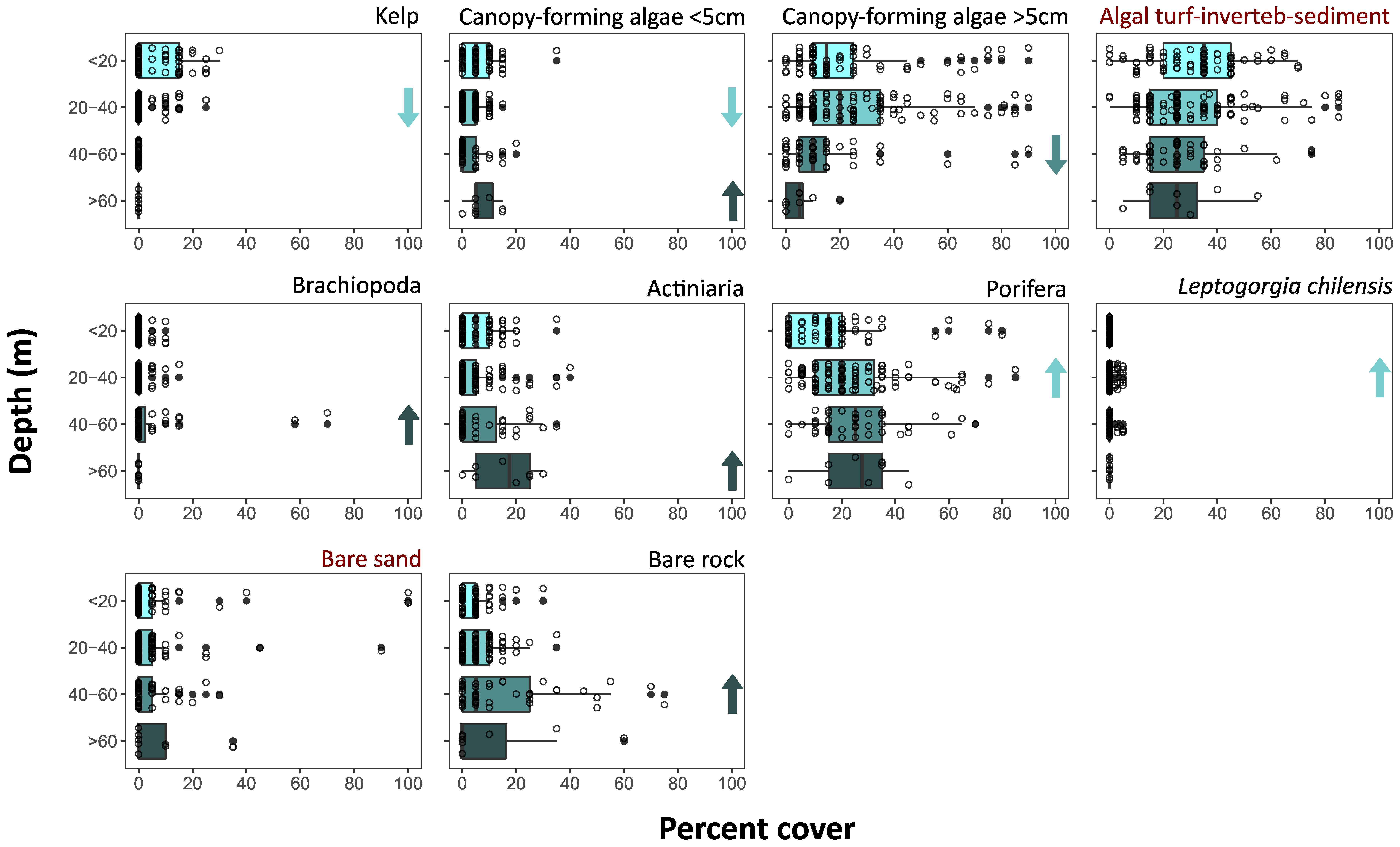
3.2. Benthic Community

A total of 13 invertebrate taxonomic entities and macrophyte groups were recognised in the quadrats, exhibiting different bathymetric distributional ranges (Figure 3). Each of these, together with bare rock and sand (not colonised substrate), individually appeared in at least 32 quadrats (of 233 analysed). The algal turf-invertebrate-sediment category, together with canopy-forming algae (two categories: <5 and >5 cm in height), almost covered the depth range studied, from 6.4 to 91 m (Figure 3, Supplementary Material Table S1). Live attached kelp Lessonia trabeculata was present from shallow depths to 39.5 m. Drifting kelp was observed only once, at 33 m in Los Vilos (10% cover). While Actiniaria and Porifera also appeared along the depth range studied, Brachiopoda disappeared at 57.7 m. Additionally, three taxa were only observed in deeper habitats, i.e., Leptogorgia chilensis (25.2–57 m), Axinella sp. (32–57.9 m), and Tetrapygus niger (25.4–47.6 m). On the other hand, mobile invertebrates, such as Stichaster striatus, Odontaster validus and Meyenaster gelatinosus, appear as shallow species, the first two slightly penetrating deeper habitats to 37.4 and 42.4 m, respectively (Figure 3, Supplementary Material Table S1).
Kelp density significantly decreased below 20 m (Figure 6, Supplementary Material Tables S6 and S7). While canopy-forming algae decreased with depth, those shorter than 5 cm increased again below 60 m deep. Increases in percent cover with depth were also found for Brachiopoda, Actiniaria, Porifera, and L. chilensis at 20, 40, or 60 m depth. An increase at 40 m was also found for bare rock.
The percent cover of benthic species shows a significant change in the community along the depth gradient, among sites, and for the interaction of the two (Table 4). The variance explained by the model was low. All sites were different from one another (F = 5.50–11.71, p = 0.001–0.025, Supplementary Material Table S8). In this case, the dispersion among sites was significant (F = 3.01, p = 0.036, Supplementary Material Table S9a), indicating that differences among sites may be caused by different within-group dispersion from the centroids. Indeed, Las Cruces showed a higher and significantly different dispersion compared to Algarrobo, El Quisco, and Los Vilos (Supplementary Material Table S9b).
The nMDS analysis of the cover data showed a high degree of overlap between the four sampled sites (Figure 7a) and among depth strata (Figure 7b).

4. Discussion

This study provides a general overview of the diversity patterns in shallow and mesophotic depths in central Chile. The patterns of species distribution show that TME here are characterised by the combination of depth-generalist species that appear at shallow and mesophotic depths together with a few species appearing from 22–32 m depth downward. These include the fish species S. oculatus, the soft coral L. chilensis (recently reviewed by Camps-Castellà et al. [57]), and the sponge A. polypoides. TME from central Chile show a lower fish richness and abundance compared to shallow waters, with less herbivores and detritivores abundance, while carnivore species are more abundant in mesophotic depths. An increase in the abundance of sponges below 20 m is very notorious.
The results suggest a transition zone at 22–32 m between shallow and mesophotic depths in central Chile. Bell et al. [9] already noted that animal-dominated communities may start to appear at 20 m in TME, shallower than the generality of MCE [2] and the typically considered (30 m) limit of the recreational SCUBA diving. Thus, although the irradiance and light penetration strongly vary between summer and winter in the study area [58], the species distributions provide more consistent limits for the upper mesophotic limits. Below 60 m, sponge, and coral species such as Axinella sp. and L. chilensis completely disappear, but the abundance of other porifera remains high and photosynthetic species, indicators of the photic zone, are still present [1,3]. This pattern suggests a second transition zone between the upper and lower mesophotic zones. This boundary depth varies in MCE from 55 m to 80 m, with 60 m the most commonly reported [2,58]. Thus, despite the great differences between tropical, subtropical, and temperate ecosystems, their contrasting richness patterns and variability in oceanographic conditions, the diversity breaks seem similar. However, these shallow, upper, and lower TME subdivisions were superficially investigated here, and this vertical zonation requires further research combining other methodologies to define the community characteristics of each depth zone.
The decrease in fish species richness and abundance with depth found in central Chile follows a general trend depicted worldwide common to MCE and TME [23,59,60]. Nevertheless, other authors have reported richness peaks at intermediate depths (30–90 m) in MCE, where shallow and deep species overlap [59]. The peak of species at intermediate depth, however, is expected in zones where the mesophotic endemics species exceed the richness of those in shallow waters, a pattern not evidenced in this study unless a considerable number of mesophotic species that cannot be adequately sampled with TUV systems remain to be discovered in the future. Another plausible explanation for the patterns of fish species richness and density found here is the topographic complexity. Since topographic complexity is not related to depth (correlation of −0.05), the general diversity trend with depth could be locally affected by the site-specific topographic complexity imposed by the habitat type. This habitat feature is important because it provides shelter, increasing fish survivorship [35,61]. Several previous studies have found a positive relationship between topographic complexity and reef fish diversity (e.g., [62]), although different approaches have been used to measure this feature. The second conspicuous pattern found in this study, matching previous reports for TME, is the decreasing abundance of herbivorous and omnivorous fishes with depth and an increasing abundance of planktivorous and carnivorous fish species (e.g., [7,60,63,64]). Exceptions to this pattern have been attributed to fishing pressure [31]. On the other hand, the increase in abundance of planktivorous fishes with depth reported in this study needs further analysis since this group is only represented by the damselfish C. crusma. The extremely high abundances found at 20–40 m might be due to the occurrence of large schools and patchy distributions known for this species [65]. Furthermore, an increase in food availability with depth, related to currents and upwelling events, has already been reported in mesophotic reefs [31,60] and may also explain the abundance of this species. C. crusma also requires rocky substrate as breeding territory for nest building [66]. Thus, the local availability of preferred substrates may be more important to explain its distribution.
A decline n herbivores, detritivores, and benthic algae follows the light attenuation with depth, which is expected to vary geographically according to water turbidity. Previous studies have reported that algae decrease below 50 m in TME [9]. We also observed this trend with a first decrease of smaller canopy-forming algae (<5 cm) below 20 m, followed by taller algae (>5 cm) below 40 m. Comparatively, taller algae strongly dominate until 60 m, where both groups persist and are equally abundant. Below 60 m, small benthic algae show a significant increase in abundance. This is also the case for sea anemones, which also appear to increase below 60 m. Nevertheless, fewer quadrats at deeper zones owing to limited visibility might be affecting these patterns.
One of the most conspicuous species in all the sites was the brachiopod. In contrast to other studies where this taxon was restricted to less than 15 m [9], it was recognised as up to 58 m here. Although there are about 15 brachiopod species described for continental Chile [67], the methodology used in this study lacks the resolution to distinguish among them. Thus, this wide depth distribution may correspond to overlapping ranges of different shallow and mesophotic species. Another contrasting pattern with other studies in TME is observed in sponges (Porifera), whose abundance peaks at 20–40 m in central Chile, while increases of abundance with depth beyond 50 m were observed in other TME [9]. However, the distinctive branching sponge A. polypoides only appears in deeper zones, between 32–58 m. On the other hand, Actiniaria and gorgonians (Octocorallia) show contrasting depth patterns in comparison with previous studies, which do not make this distinction within cnidarians [9]. Thus, while gorgonians peak at 20–40 m, anemones show similar abundances through the depth gradient (up to 40 percent cover).
The replacement of the shallow kelp forests by the gorgonian L. chilensis and porifera as A. polypoides below 20 m suggests the relevance of animal forests in TME. These invertebrate species collectively provide habitat and offer benthic complexity, generating refuges and food for other species [68,69]. In fact, a variety of gastropods, crustaceans, and other invertebrates are frequently observed in colonies of these species (personal observations). Contrary to what has been reported for similar species in other regions, as in the case of Paramuricea clavata in the Mediterranean [9], no dense aggregations of L. chilensis were observed at mesophotic depths. Nevertheless, the extent to which corals and sponges contribute to habitat complexity in TME of central Chile escapes the scope of this work. We have no data to conclude if the sparseness of these animals is or is not the result of damaging activities, such as fishing gear or other activities producing mechanical damages, including anchorages or divers [69]. Nonetheless, it is important to remark that these species have a slow-growing and long-lived nature, making them highly vulnerable to recovery after mortality events which might have long-lasting effects on the communities associated with animal forests [69]. For this reason, delineating the areas where these species form dense assemblages is essential to protect these animal forests, which may sustain commercially important fishes and other ecosystem services.
Despite the recognised constraints associated with the use of towed underwater cameras, it was possible to depict general diversity patterns for TME in central Chile. Among these constraints, the difficulties to manoeuvre the camera underwater might have affected the possibility to identify some specimens, underestimating the abundance and depth ranges. Additionally, the size of the quadrants (0.25 m2) might have limited the abundance of some mobile species. For instance, the black sea urchin T. niger was found below 25 m, but this is a common intertidal species (e.g., [70]). Thus, the shallow depth limit is underestimated. However, the deeper occurrence extends its known depth range from 40 m [70] to 47.6 m. On the other hand, the attained taxonomic resolution for the benthic community is comparable to previous studies in TME [9]. Overall, broad categories, such as canopy-forming algae (<5 cm/>5 cm) and “algal turf-invertebrate-sediment”, which appeared throughout the entire depth range, definitively require a finer resolution. Only then, the true number of taxa restricted to mesophotic depths will be revealed, as new species are also continuously being discovered in other ME [2,7]. Other considerations are related to the time of the day that the data was collected (e.g., limitations to detect nocturnal species), cryptic species and habitats (e.g., sheltered congers), or attraction/avoidance to the camera (mobile species react to the presence of the camera).
In general, the multivariate representation of both fish and the benthic assemblages shows that the community composition does not strongly differ among locations or depths. This means that there are minor environmental effects among sites or that these do not strongly affect the community structure. Globally, the community composition in TME has been reported to be different between depths but not among regions [9]. Although the spatial scale differs, this points to generalities among TME worldwide, and even MCE. Regarding depth, there is not enough evidence to discard its influence on the community composition here. This data has shown general patterns characteristic of TME and distinctive from shallow waters, and further research in combination with other methodologies (e.g., BRUVs, ROVs, eDNA, acoustic monitoring or video transects by technical diving) will be decisive to understand what extent communities change with depth in TME from central Chile.
In conclusion, this study focusing on TME from central Chile allows the first description of marine communities from shallow to 90 m depth. The relevance of increasing research efforts in these ecosystems, and the Southeastern Pacific in particular, is notably critical, considering the increasing anthropogenic effects that other studies have already stressed affect them.

Supplementary Materials

The following supporting information can be downloaded at: https://www.mdpi.com/article/10.3390/d15030360/s1, Figure S1: Images extracted from the TUV. Some of the main taxa observed in the TUV are pointed on each image. (a) Kelp. Las Cruces, 12.9 m; (b) Actiniaria and Porifera. Los Vilos, 47.6 m. (c) Brachiopoda, Porifera, and Sebastes oculatus. El Quisco, 50.7 m. (d) Porifera. Las Cruces, 33.5 m. (e) Canopy-forming algae > 5 cm. El Quisco, 9.9 m. (f) Stichaster striatus and Chromis crusma. Algarrobo, 25.2 m. (g) Leptogorgia chilensis. El Quisco, 38.7 m. (h) Axinella sp. El Quisco, 50.5 m; Figure S2: Density distribution of sampled depth at each site. Vertical lines represent the median depth sampled at each site (Algarrobo 31.3 m, N = 203; El Quisco 28.8 m, N = 124 Las Cruces 28.7 m, N = 192; Los Vilos 42.8 m, N = 259). Observations (N) correspond to 30 s intervals recorded by the GPS; Table S1: All sites and by-site depth range of fish and benthic taxa, including fish trophic categories. Empty cells correspond to taxon absence, while single depth values are single occurrences. Invert.: invertebrates; Figure S3: Species accumulation curves for the four sampled sites: (a) Algarrobo, (b) El Quisco, (c) Las Cruces and (d) Los Vilos; Table S2: Kruskal–Wallis rank sum test for the density of fish species and trophic categories between depth strata: <20 m (N = 33), 20–40 m (N = 44), 40–60 m (N = 27), >60 m (N = 16). Only species with more than two occurrences on each depth section (N = 120) are included, while all recognised fish taxa were grouped in trophic categories. p-values < 0.05 are highlighted in bold; Table S3: Pairwise comparison of fish species and trophic categories that showed a significantly different density among depth bands (<20 m, 20–40 m, 40–60 m, >60 m) using a Bonferroni´s correction. p-values < 0.05 are highlighted in bold; Table S4: Pairwise comparison of the fish community across sites using PERMANOVA (999 permutations). p-values < 0.05 are highlighted in bold; Table S5: Permutation test for homogeneity of multivariate dispersions on the fish community across sites. Table S6: Kruskal–Wallis rank sum test for the percentage cover data between depth bands: <20 m (N = 73), 20–40 m (N = 109), 40–60 m (N = 47), >60 m (N = 8). p-values < 0.05 highlighted in bold. Inverteb: invertebrates; Table S7: Pairwise comparison of the percentage cover data that showed a significantly different abundance between depth bands (<20 m, 20–40 m, 40–60 m, >60 m) using a Bonferroni´s correction. p-values < 0.05 are highlighted in bold; Table S8: Pairwise comparison of the percent cover data across sites using PERMANOVA (999 permutations). p-values < 0.05 are highlighted in bold. Table S9a: Permutation test for homogeneity of multivariate dispersions on the percent cover data of the benthic community across sites. p-value < 0.05 highlighted in bold; Table S9b: Pairwise comparison for homogeneity of multivariate dispersions on the percent cover data of the benthic community across sites. Observed p-value below diagonal, permuted p-value above diagonal. p-values < 0.05 in bold.

Author Contributions

Conceptualization, A.P.-M., E.A.W., R.A.-I., V.G., and M.F.; methodology, A.N.C., A.P.-M., E.A.W., R.A.-I., V.G., and M.F.; formal analysis, A.N.C.; writing—original draft preparation, A.N.C.; writing—review and editing, A.N.C., A.P.-M., E.A.W., R.B., S.A.N., and M.F.; supervision, A.N.C. and M.F.; project administration, M.F. All authors have read and agreed to the published version of the manuscript.

Funding

This research was funded by Núcleo Milenio grant number ICM_NCN19_056. APM was funded by Fondecyt regular #1210216.

Institutional Review Board Statement

Not applicable.

Informed Consent Statement

Not applicable.

Data Availability Statement

Not applicable.

Acknowledgments

We acknowledge Katherine Espinoza and Carlos Molinet for their advice on using the towed underwater video cameras. We especially thank Ainara Aguilar for her collaboration on field trips. Finally, we acknowledge Alexandre Génin for the helpful discussions.

Conflicts of Interest

The authors declare no conflict of interest.

References

  1. Cerrano, C.; Bastari, A.; Calcinai, B.; Di Camillo, C.; Pica, D.; Puce, S.; Valisano, L.; Torsani, F. Temperate mesophotic ecosystems: Gaps and perspectives of an amerging conservation challenge for the Mediterranean Sea. Eur. Zool. J. 2019, 86, 370–388. [Google Scholar] [CrossRef] [Green Version]
  2. Pyle, R.L.; Copus, J.M. Mesophotic coral ecosystems: Introduction and overview. In Mesophotic Coral Ecosystems; Loya, Y., Puglise, K.A., Bridge, T.C.L., Eds.; Springer: Cham, Switzerland, 2019; pp. 3–27. [Google Scholar]
  3. Turner, J.A.; Andradi-Brown, D.A.; Gori, A.; Bongaerts, P.; Burdett, H.L.; Ferrier-Pagès, C.; Voolstra, C.R.; Weinstein, D.K.; Bridge, T.C.L.; Costantini, F.; et al. Key questions for research and conservation of mesophotic coral ecosystems and temperate mesophotic ecosystems. In Mesophotic Coral Ecosystems; Loya, Y., Puglise, K.A., Bridge, T.C.L., Eds.; Springer: Cham, Switzerland, 2019; pp. 989–1003. [Google Scholar]
  4. Eyal, G.; Pinheiro, H.T. Mesophotic ecosystems: The link between shallow and deep-sea habitats. Diversity 2020, 12, 411. [Google Scholar] [CrossRef]
  5. Puglise, K.A.; Hinderstein, L.M.; Marr, J.C.A.; Dowgiallo, M.J.; Martinez, F.A. Mesophotic Coral Ecosystems Research Strategy. In Proceedings of the International Workshop to Prioritize Research and Management Needs for Mesophotic Coral Ecosystems, Jupiter, FL, USA, 12–15 July 2008; NOAA/National Centers for Coastal Ocean Science: Silver Spring, MD, USA; p. 24. [Google Scholar]
  6. Hinderstein, L.; Marr, J.C.A.; Martinez, F.A.; Dowgiallo, M.J.; Puglise, K.A.; Pyle, R.L.; Zawada, D.G.; Appeldoorn, R. Theme section on “mesophotic coral ecosystems: Characterization, ecology, and management”. Coral Reefs 2010, 29, 247–251. [Google Scholar] [CrossRef] [Green Version]
  7. Rocha, L.A.; Pinheiro, H.T.; Shepherd, B.; Papastamatiou, Y.P.; Luiz, O.J.; Pyle, R.L.; Bongaerts, P. Mesophotic coral ecosystems are threatened and ecologically distinct from shallow water reefs. Science 2018, 361, 281–284. [Google Scholar] [CrossRef] [Green Version]
  8. Cerrano, C.; Danovaro, R.; Gambi, C.; Pusceddu, A.; Riva, A.; Schiaparelli, S. Gold coral (Savalia savaglia) and gorgonian forests enhance benthic biodiversity and ecosystem functioning in the mesophotic zone. Biodivers. Conserv. 2010, 19, 153–167. [Google Scholar] [CrossRef] [Green Version]
  9. Bell, J.J.; Micaroni, V.; Harris, B.; Strano, F.; Broadribb, M.; Rogers, A. Global status, impacts, and management of rocky temperate mesophotic ecosystems. Conserv. Biol. 2022, e13945. [Google Scholar] [CrossRef]
  10. Micaroni, V.; McAllen, R.; Turner, J.; Strano, F.; Morrow, C.; Picton, B.; Harman, L.; Bell, J.J. Vulnerability of Temperate Mesophotic Ecosystems (TMEs) to environmental impacts: Rapid ecosystem changes at Lough Hyne Marine Nature Reserve, Ireland. Sci. Total Environ. 2021, 789, 147708. [Google Scholar] [CrossRef]
  11. Shepherd, B.; Phelps, T.; Pinheiro, H.T.; Pérez-Matus, A.; Rocha, L.A. Plectranthias ahiahiata, a new species of perchlet from a mesophotic ecosystem at Rapa Nui (Easter Island) (Teleostei, Serranidae, Anthiadinae). ZooKeys 2018, 762, 105–116. [Google Scholar] [CrossRef] [Green Version]
  12. Sheperd, B.; Pinheiro, H.T.; Phelps, T.; Pérez-Matus, A.; Rocha, L.A. Luzonichthys kiomeamea (Teleostei: Serranidae: Anthiadinae), a new species from a mesophotic coral ecosystem of Rapa Nui (Easter Island). J. Ocean Sci. Found. 2019, 33, 17–27. [Google Scholar]
  13. Easton, E.E.; Gorny, M.; Mecho, A.; Sellanes, J.; Gaymer, C.F.; Spalding, H.L.; Aburto, J. Chile and the Salas y Gómez Ridge. In Mesophotic Coral Ecosystems; Loya, Y., Puglise, K.A., Bridge, T.C.L., Eds.; Springer: Cham, Switzerland, 2019; pp. 477–490. [Google Scholar]
  14. Hoeksema, B.W.; Sellanes, J.; Easton, E.E. A high-latitude, mesophotic Cycloseris field at 85 m depth off Rapa Nui (Easter Island). Bull. Mar. Sci. 2019, 95, 101–102. [Google Scholar] [CrossRef]
  15. Shepherd, B.; Pinheiro, H.T.; Phelps, T.A.Y.; Easton, E.E.; Pérez-Matus, A.; Rocha, L.A. A New Species of Chromis (Teleostei: Pomacentridae) from Mesophotic Coral Ecosystems of Rapa Nui (Easter Island) and Salas y Gómez, Chile. Copeia 2020, 108, 326–332. [Google Scholar] [CrossRef]
  16. Sellanes, J.; Gorny, M.; Zapata-Hernández, G.; Álvarez, G.; Muñoz, P.; Tala, F. A new threat to local marine biodiversity: Filamentous mats proliferating at mesophotic depths off Rapa Nui. PeerJ 2021, 9, e12052. [Google Scholar] [CrossRef]
  17. Mecho, A.; Dewitte, B.; Sellanes, J.; van Gennip, S.; Easton, E.E.; Gusmao, J.B. Environmental drivers of mesophotic echinoderm assemblages of the southeastern Pacific Ocean. Front. Mar. Sci. 2021, 8, 574780. [Google Scholar] [CrossRef]
  18. Försterra, G.; Häussermann, V.; Laudien, J. Animal Forests in the Chilean fjords: Discoveries, perspectives and threats in shallow and deep waters. In Marine Animal Forests; Rossi, S., Bramanti, L., Gori, A., Orejas, C., Eds.; Springer: Cham, Switzerland, 2016. [Google Scholar]
  19. Gorny, M.; Easton, E.E.; Sellanes, J. First record of black corals (Antipatharia) in shallow coastal waters of northern Chile by means of underwater video. Lat. Am. J. Aquat. Res. 2018, 46, 457–460. [Google Scholar] [CrossRef]
  20. Holstein, D.M.; Fletcher, P.; Groves, S.H.; Smith, T.B. Ecosystem services of mesophotic coral ecosystems and a call for better accounting. In Mesophotic Coral Ecosystems; Loya, Y., Puglise, K.A., Bridge, T.C.L., Eds.; Springer: Cham, Switzerland, 2019; pp. 943–956. [Google Scholar]
  21. Gómez, F.A.; Spitz, Y.H.; Batchelder, H.P.; Correa-Ramírez, M.A. Intraseasonal patterns in coastal plankton biomass off central Chile derived from satellite observations and a biochemical model. J. Mar. Syst. 2017, 174, 106–118. [Google Scholar] [CrossRef]
  22. Thiel, M.; Macaya, E.C.; Acuña, E. The Humboldt Current system of northern and central Chile. Oceanogr. Mar. Biol. 2007, 45, 195–344. [Google Scholar]
  23. Kahng, S.E.; Garcia-Sais, J.R.; Spalding, H.L.; Brokovich, E.; Wagner, D.; Weil, E.; Hinderstein, L.; Toonen, R.J. Community ecology of mesophotic coral reef ecosystems. Coral Reefs 2010, 29, 255–275. [Google Scholar] [CrossRef]
  24. Glynn, P.W. Coral reef bleaching: Facts, hypotheses and implications. Glob. Chang. Biol. 1996, 2, 495–509. [Google Scholar] [CrossRef]
  25. Asher, J.; Williams, I.D.; Harvey, E.S. Mesophotic depth gradients impact reef fish assemblage composition and functional group partitioning in the main Hawaiian Islands. Front. Mar. Sci. 2017, 4, 98. [Google Scholar] [CrossRef] [Green Version]
  26. Voerman, S.E. Ecosystem engineer morphological traits and taxon identity shape biodiversity across the euphotic-mesophotic transition. Proc. R. Soc. B. 2022, 289, 20211834. [Google Scholar] [CrossRef]
  27. Lesser, M.P.; Slattery, M.; Leichter, J.J. Ecology of mesophotic coral reefs. J. Exp. Mar. Biol. Ecol. 2009, 375, 1–8. [Google Scholar] [CrossRef]
  28. Bongaerts, P.; Ridgway, T.; Sampayo, E.M.; Hoegh-Guldberg, O. Assessing the “deep-reef refugia” hypothesis: Focus on Caribbean reefs. Coral Reefs 2010, 29, 309–327. [Google Scholar] [CrossRef]
  29. Loya, Y.; Eyal, G.; Treibitz, T.; Lesser, M.P.; Appeldoorn, R. Theme section on mesophotic coral ecosystems: Advances in knowledge and future perspectives. Coral Reefs 2016, 35, 1–9. [Google Scholar] [CrossRef] [Green Version]
  30. Sih, T.L.; Cappo, M.; Kingsford, M.J. Deep-reef fish assemblages of the Great Barrier Reef shelf-break (Australia). Sci. Rep. 2017, 7, 10886. [Google Scholar] [CrossRef] [PubMed] [Green Version]
  31. Pinheiro, H.T.; Goodbody-Grinley, G.; Jessup, M.E.; Shepherd, B.; Chequer, A.D.; Rocha, L.A. Upper and lower mesophotic coral reef fish communities evaluated by underwater visual censuses in two Caribbean locations. Coral Reefs 2016, 35, 139–151. [Google Scholar] [CrossRef] [Green Version]
  32. Bridge, T.C.L.; Hughes, T.P.; Guinotte, J.M.; Bongaerts, P. Call to protect all coral reefs. Nat. Clim. Chang. 2013, 3, 528–530. [Google Scholar] [CrossRef] [Green Version]
  33. Smith, T.B.; Glynn, P.W.; Maté, J.L.; Toth, L.T.; Gyory, J. A depth refugium from catastrophic coral bleaching prevents regional extinction. Ecology 2014, 95, 1663–1673. [Google Scholar] [CrossRef] [PubMed] [Green Version]
  34. Pérez-Matus, A.; Neubauer, P.; Shima, J.S.; Rivadeneira, M.M. Reef fish diversity across the Temperate South Pacific Ocean. Front. Ecol. Evol. 2022, 10, 768707. [Google Scholar] [CrossRef]
  35. Carbines, G.; Cole, R.C. Using a remote drift underwater video (DUV) to examine dredge impacts on demersal fishes and benthic habitat complexity in Foveaux Strait, Southern New Zealand. Fish. Res. 2009, 96, 230–237. [Google Scholar] [CrossRef]
  36. Schneider, C.A.; Rasband, W.S.; Eliceiri, K.W. NIH Image to ImageJ: 25 years of image analysis. Nat. Methods 2012, 9, 671–675. [Google Scholar] [CrossRef]
  37. Foster, M.S.; Harrold, C.; Hardin, D.D. Point vs. photo quadrat estimates of the cover of sessile marine organisms. J. Exp. Mar. Biol. Ecol. 1991, 146, 193–203. [Google Scholar] [CrossRef]
  38. Kohler, K.E.; Gill, S.M. Coral Point Count with Excel extensions (CPCe): A visual basic program for the determination of coral and substrate coverage using random point count methodology. Comput. Geosci. 2006, 32, 1259–1269. [Google Scholar] [CrossRef]
  39. Gotelli, N.J.; Colwell, R.K. Estimating Species Richness. In Biological Diversity: Frontiers in Measurement and Assessment; Magurran, A.E., McGill, B.J., Eds.; Oxford University Press: New York, NY, USA, 2011; Chapter 4; pp. 39–54. [Google Scholar]
  40. Chao, A.; Shen-Ming, L. Estimating the number of classes via sample coverage. JASA 1992, 87, 210–217. [Google Scholar] [CrossRef]
  41. Dormann, C.F.; Elith, J.; Bacher, S.; Buchmann, C.; Carl, G.; Carré, G.; Marquéz, J.R.G.; Gruber, B.; Lafourcade, B.; Leitão, P.J.; et al. Collinearity: A review of methods to deal with it and a simulation study evaluating their performance. Ecography 2013, 36, 27–46. [Google Scholar] [CrossRef]
  42. Anderson, M.J. A new method for non-parametric multivariate analysis of variance. Austral Ecol. 2001, 26, 32–46. [Google Scholar]
  43. Kruskal, J.B.; Wish, M. Multidimensional Scaling; Sage Publications: Thousand Oaks, CA, USA, 1978; p. 93. [Google Scholar]
  44. R Core Team. R: A Language and Environment for Statistical Computing. Vienna, Austria: R Foundation for Statistical Computing. 2019. Available online: https://www.r-project.org (accessed on 25 January 2023).
  45. Delignette-Muller, M.L.; Dutang, C. Fitdistrplus: An R package for fitting distributions. J. Stat. Softw. 2015, 64, 1–34. [Google Scholar] [CrossRef] [Green Version]
  46. Wei, T.; Simko, V. R Package ‘Corrplot’: Visualization of a Correlation Matrix (Version 0.92). 2021. Available online: https://github.com/taiyun/corrplot (accessed on 25 January 2023).
  47. Bates, D.; Maechler, M.; Bolker, B.; Walker, S. Fitting linear mixed-effects models using lme4. J. Stat. Softw. 2015, 67, 1–48. [Google Scholar] [CrossRef]
  48. Barton, K. MuMIn: Multi-Model Inference. R package Version 1.46.0. 2022. Available online: https://CRAN.R-project.org/package=MuMIn (accessed on 25 January 2023).
  49. Korner-Nievergelt, F.; Roth, T.; von Felten, S.; Guelat, J.; Almasi, B.; Korner-Nievergelt, P. Bayesian Data Analysis in Ecology Using Linear Models with R, BUGS and Stan; Elsevier: Amsterdam, The Netherlands, 2015. [Google Scholar]
  50. Halekoh, U.; Højsgaard, S. A Kenward-Roger approximation and parametric bootstrap methods for tests in linear mixed models—The R package pbkrtest. J. Stat. Softw. 2014, 59, 1–30. [Google Scholar] [CrossRef] [Green Version]
  51. Haritg, F. DHARMa: Residual Diagnostics for Hierarchical (Multi-Level/Mixed) Regression Models. R Package Version 0.4.6. 2022. Available online: https://CRAN.R-project.org/package=DHARMa (accessed on 25 January 2023).
  52. Wickham, H. Ggplot2: Elegant Graphics for Data Analysis; Springer: New York, NY, USA, 2016. [Google Scholar]
  53. Lüdecke, D. Ggeffects: Tidy Data Frames of Marginal Effects from Regression Models. J. Open Source Softw. 2018, 3, 772. [Google Scholar] [CrossRef] [Green Version]
  54. Vavrek, M.J. Fossil: Palaeoecological and palaeogeographical analysis tools (version 0.4.0). Palaeontol. Electron. 2011, 14, 1. [Google Scholar]
  55. Oksanen, J.; Blanchet, F.G.; Kindt, R.; Legendre, P.; O’hara, R.B.; Simpson, G.L.; Solymos, P.; Stevens, M.H.H.; Wagner, H. Vegan: Community Ecology Package. R Package Version 2.6-2. 2022. Available online: https://CRAN.R-project.org/package=vegan (accessed on 25 January 2023).
  56. Hervé, M. RVAideMemoire: Testing and Plotting Procedures for Biostatistics. R Package Version 0.9-81-2. Available online: https://CRAN.R-project.org/package=RVAideMemoire (accessed on 25 January 2023).
  57. Camps-Castellà, J.; Breedy, O.; Vera-Escalona, I.; Vargas, S.; Silva, F.; Hinojosa, I.A.; Prado, P.; Brante, A. Distribution and divergence of shallow and upper mesophotic cold-water gorgonians (Octocorallia: Gorgoniidae) in Chilean coasts, with the description of a new species. In Proceedings of the VIII International Symposium on Marine Sciences, Las Palmas de Gran Canaria, Spain, 6–8 July 2022; p. 198. [Google Scholar]
  58. Montecino, V.; Pizarro, G. Phytoplankton acclimation and spectral penetration of UV irradiance off the central Chilean coast. Mar. Ecol. Prog. Ser. 1995, 121, 261–269. [Google Scholar] [CrossRef] [Green Version]
  59. Pyle, R.L.; Kosaki, R.K.; Pinheiro, H.T.; Rocha, L.A.; Whitton, R.K.; Copus, J.M. Fishes: Biodiversity. In Mesophotic Coral Ecosystems; Loya, Y., Puglise, K.A., Bridge, T.C.L., Eds.; Springer: New York, NY, USA, 2019; pp. 749–777. [Google Scholar]
  60. Thresher, R.E.; Colin, P.L. Trophic structure, diversity and abundance of fishes of the deep reef (30–300 m) at Enewetak, Marshall Islands. Bull. Mar. Sci. 1986, 38, 253–272. [Google Scholar]
  61. Connell, S.D.; Jones, G.P. The influence of habitat complexity on postrecruitment processes in a temperate reef fish population. J. Exp. Mar. Biol. Ecol. 1991, 151, 271–294. [Google Scholar] [CrossRef]
  62. Friedlander, A.M.; Brown, E.K.; Jokiel, P.L.; Smith, W.R.; Rodgers, K.S. Effects of habitat, wave exposure, and marine protected area status on coral reef fish assemblages in the Hawaiian archipelago. Coral Reefs 2003, 22, 291–305. [Google Scholar] [CrossRef]
  63. Bejarano, I.; Appeldoorn, R.S.; Nemeth, M. Fishes associated with mesophotic coral ecosystems in La Parguera, Puerto Rico. Coral Reefs 2014, 33, 313–328. [Google Scholar] [CrossRef]
  64. Stefanoudis, P.V.; Rivers, M.; Smith, S.R.; Schneider, C.W.; Wagner, D.; Ford, H.; Rogers, A.D.; Woodall, L.C. Low connectivity between shallow, mesophotic and rariphotic zone benthos. R. Soc. Open Sci. 2019, 6, 190958. [Google Scholar] [CrossRef] [PubMed] [Green Version]
  65. Pérez-Matus, A.; Ferry-Graham, L.; Cea, A.; Vásquez, J. Community structure of temperate reef fishes in kelp-dominated subtidal habitats of northern Chile. Mar. Fresh. Res. 2007, 58, 1069–1085. [Google Scholar] [CrossRef]
  66. Navarrete-Fernández, T.; Landaeta, M.F.; Bustos, C.A.; Pérez-Matus, A. Nest building and description of parental care behavior in a temperate reef fish, Chromis crusma (Pisces: Pomacentridae). Rev. Chil. Hist. Nat. 2014, 87, 30. [Google Scholar] [CrossRef] [Green Version]
  67. Lee, M.R.; Hermosilla, C.; Castilla, J.C.; Fernández, M.; Clarke, M.; González, C.; Prado, L.; Rozbaczylo, N.; Valdovinos, C. Free-living benthic marine invertebrates in Chile. Rev. Chil. Hist. Nat. 2008, 81, 51–67. [Google Scholar] [CrossRef] [Green Version]
  68. Coni, E.O.C.; Ferreira, C.M.; de Moura, R.L.; Meirelles, P.M.; Kaufman, L.; Francini-Filho, R.B. An evaluation of the use of branching fire-corals (Millepora spp.) as refuge by reef fish in the Abrolhos Bank, eastern Brazil. Environ. Biol. Fishes 2013, 96, 45–55. [Google Scholar] [CrossRef]
  69. Ponti, M.; Turicchia, E.; Ferro, F.; Cerrano, C.; Abbiati, M. The understorey of gorgonian forests in mesophotic temperate reefs. Aquat. Conserv. Mar. Freshw. Ecosyst. 2018, 28, 1153–1166. [Google Scholar] [CrossRef]
  70. Rodríguez, S.R. Consumption of drift kelp by intertidal populations of the sea urchin Tetrapygus niger on the central Chilean coast: Possible consequences at different ecological levels. Mar. Ecol. Prog. Ser. 2003, 251, 141–151. [Google Scholar] [CrossRef] [Green Version]
Figure 1. Towed underwater video transects performed at four sites: Los Vilos, Algarrobo, El Quisco and Las Cruces.
Diversity 15 00360 g001
Figure 2. Conditional curves depicting the predicted fish density (a,b) and richness (c,d) by the GLMM and actual values (coloured dots). Depth and topographic complexity were standardised to have zero mean and unit standard deviation. Covariables not represented in each graph (fixed and random effects) were held at zero in the predictions. For fish density (a,b), the transect surface is held at 194.54 m2 (offset mean), and fish density is obtained by dividing predicted fish abundance by 194.54. GLMM for fish richness does not include offset. N = 120.
Diversity 15 00360 g002
Figure 3. Violin plots showing taxa and fish trophic categories occurrences with depth, based on number of sections where each taxon appeared in the case of fish species and fish trophic categories, and number of 0.25 m2 quadrats for benthic taxa. Only fish taxa with more than two occurrences on depth sections (N = 120) are individually represented, while all fish taxa were grouped in trophic categories. Invert: invertebrates.
Diversity 15 00360 g003
Figure 4. Density of fish species and trophic categories in depth strata. Points are taxa occurrences on video sections; on boxplots: vertical lines indicate median value; boxplot hinges indicate first and third quartiles; boxplot whiskers indicate largest and lower values no further than 1.5× inter-quartile range from the respective hinge; and data beyond the whiskers indicate outliers. Taxa in red highlight non-significant differences between depth strata (Kruskal–Wallis rank sum test, p-value < 0.05). Arrows indicate significant increases or decreases regarding the immediate shallower depth category as given by pairwise comparisons.
Diversity 15 00360 g004
Figure 5. Non-metric multidimensional scaling (nMDS) plot using a Bray–Curtis dissimilarity matrix (dimensions = 2, stress = 0.10, Shepard plot non-metric R2 = 0.99). (a) Sites. (b) Depth strata. Ellipses include 95% of the data for each group. Dots with black borders and a more intense colour indicate the centroids for each site.
Diversity 15 00360 g005
Figure 6. Percent cover of benthic taxa and bare sand or rock (available for colonisation) in depth strata. Points represent occurrences on quadrats; on boxplots: vertical lines indicate median value; boxplot hinges indicate first and third quartiles; boxplot whiskers indicate largest and lower values no further than 1.5× inter-quartile range from the respective hinge; and data beyond the whiskers indicate outliers. Red highlights non-significant differences between depth strata (Kruskal–Wallis rank sum test, p-value < 0.05). Arrows indicate significant increases or decreases regarding the immediate shallower depth category as given by pairwise comparisons.
Diversity 15 00360 g006
Figure 7. Non-metric multidimensional scaling (nMDS) plot using a Bray–Curtis dissimilarity matrix (dimensions = 3, stress = 0.13, Shepard plot non-metric R2 = 0.98). (a) Sites. (b) Depth strata. Ellipses include 95% of the data for each group. Dots with black borders and a more intense colour indicate the centroids for each site.
Diversity 15 00360 g007
Table 1. Sampled sites (see Figure 1 for location details), sampled area (m2), and number of transects performed. For each dataset, the total observations (N) and sampled depth range (m) are specified. Observations correspond to video sections for reef fish species and 0.25 m2 quadrats for the benthic community. Depth for reef fish species corresponds to the mean depth of the video section.
SiteAreaTransectsReef Fish SpeciesBenthic Community
NDepthNDepth
Los Vilos8557.206487.0–88.9846.4–91
Algarrobo5229.2832321.8–68.15018–50.5
El Quisco2631.077228.4–63.9488–50.7
Las Cruces6927.1322711.9–60.95112.3–55.8
Total23,344.68181207.0–88.92336.4–91
Table 2. Summary of the final GLMM fits modelling fish abundance and fish richness. Depth, topographic complexity, and sampled area are standardised explanatory variables. Transect (N = 18) and site (N = 4) are nested random effects in both models. Std. Error: standard error, Std. Dev.: standard deviation, R2m: marginal pseudo-r-squared, R2c: conditional pseudo-r-squared. N = 120. p-values < 0.05 highlighted in bold.
Fish Abundance
Negative Binomial Distribution (thetha = 1.23)
Fixed effectsEstimateStd. Error2.5%97.5%z-valuep-value
(Intercept)
Depth
Topographic complexity
−3.30
−0.57
0.97
0.22
0.15
0.13
−6.39
−0.05
0.69
−4.21
−0.01
1.19
−14.73
−3.73
7.45
<0.001
<0.001
<0.001
Random effectsVarianceStd. Dev.
Transect: site
Site
0.22
0.09
0.47
0.31
R2m 0.519, R2c 0.640
Overdispersion 1.02
Fish richness
Poisson Distribution
Fixed effectsEstimateStd. Error2.5%97.5%z-valuep-value
(Intercept)
Sampled area
Depth
Topographic complexity
0.64
0.03
−0.35
0.36
0.08
0.08
0.09
0.09
0.47
−0.12
−0.52
0.21
0.83
0.19
−0.17
0.53
8.07
0.43
−3.98
4.19
<0.001
0.668
<0.001
<0.001
Random effectsVarianceStd. Dev.
Transect: site
Site
0.003
0.001
0.054
0.031
R2m 0.356, R2c 0.362
Overdispersion 0.85
Table 3. Permutational multivariate analysis of variance (PERMANOVA, 999 permutations, based on a Bray–Curtis dissimilarity matrix) for the reef fish community. p-values < 0.05 highlighted in bold.
DfSum SqR2Fp
Depth14.020.1318.370.001
Site31.870.062.840.003
Topographic complexity12.710.0912.380.001
depth:site31.510.052.300.010
Topographic complexity:site30.620.020.940.531
Residuals9119.900.65
Total10230.611.00
Table 4. Permutational multivariate analysis of variance (PERMANOVA, 999 permutations, based on a Bray–Curtis dissimilarity matrix) for the percent cover of benthic species. p-values < 0.05 highlighted in bold.
DfSum SqR2Fp
Depth11.730.0514.880.001
Site32.850.088.160.001
depth:site32.850.088.170.001
Residuals22926.650.78
Total23634.081.00
Disclaimer/Publisher’s Note: The statements, opinions and data contained in all publications are solely those of the individual author(s) and contributor(s) and not of MDPI and/or the editor(s). MDPI and/or the editor(s) disclaim responsibility for any injury to people or property resulting from any ideas, methods, instructions or products referred to in the content.

