Measured Effects of Anthropogenic Development on Vertebrate Wildlife Diversity

Smallwood, K. Shawn; Smallwood, Noriko L.

doi:10.3390/d15101037

Open AccessEditor’s ChoiceArticle

Measured Effects of Anthropogenic Development on Vertebrate Wildlife Diversity

by

K. Shawn Smallwood

^*

and

Noriko L. Smallwood

Independent Researcher, 3108 Finch Street, Davis, CA 95616, USA

^*

Author to whom correspondence should be addressed.

Diversity 2023, 15(10), 1037; https://doi.org/10.3390/d15101037

Submission received: 26 July 2023 / Revised: 18 September 2023 / Accepted: 21 September 2023 / Published: 27 September 2023

(This article belongs to the Special Issue Diversity and Distribution of Wildlife Species in Relation to Human Impacts)

Download

Browse Figures

Review Reports Versions Notes

Abstract

:

A major driver of the declining biodiversity is landcover change leading to loss of habitat. Many studies have estimated large-scale declines in biodiversity, but loss of biodiversity at a local scale due to the immediate effects of development has been poorly studied. California, in particular, is a biodiversity hotspot and has rapidly developed; thus, it is important to understand the effects of development on wildlife in the State. Here, we conducted reconnaissance surveys—a type of survey often used by consulting biologists in support of environmental review of proposed projects—to measure changes in the relative abundance and richness of vertebrate species in response to urban development. We completed 2 reconnaissance surveys at each of 52 control sites that remained undeveloped at the times of both surveys, and at each of 26 impact sites that had been developed by the time of the second survey. We completed the surveys as part of a before–after, control–impact (BACI) experimental design. Our main interest was the interaction effect between the before–after phases and the control–impact treatment levels, or the impact of development. After controlling for survey duration, we also tested for the effects of the number of years intervening the surveys in the before and after phases, project area size, latitude, degree of connectedness to adjacent open space, and whether the site was a redevelopment site, infill, or not infill. After development, the average number of vertebrate wildlife species we detected declined by 48% within the project area, and by 66% within the bounds of the project sites. Further, the average number of vertebrate animals we counted declined by 90% within the project area, and 89% within the bounds of the project sites. Development impacts measured by the mean number of species detected per survey were greatest for amphibians (−100%), followed by mammals (−86%), grassland birds (−75%), raptors (−53%), special-status species (−49%), all birds as a group (−48%), non-native birds (−44%), and synanthropic birds (−28%). Our results indicated that urban development substantially reduced vertebrate species richness and numerical abundance, even after richness and abundance had likely already been depleted by the cumulative effects of loss, fragmentation, and degradation of habitat in the urbanizing environment. Monitoring is needed in and around urbanizing areas to measure the cumulative effects of urbanization, and so are conservation measures to mitigate the effects of urbanization.

Keywords:

BACI experiment; birds; California; development; reconnaissance survey; species richness; urbanization; vertebrate wildlife

1. Introduction

Urbanization has been defined as “the process of human settlement that gradually transforms uninhabited wildlands into lands including some degree of relatively permanent human presence” [1]. Urban growth profoundly affects the availability and condition of natural resources, and within its immediate area it often fragments and degrades habitat and simplifies biological species composition [2], as well as homogenizes species composition of plants [3], arthropods [4,5,6], birds [7,8,9,10,11], and land-cover composition, landscape structure, and ecosystem functions [12]. Urban areas also reduce avian taxonomic diversity [13]. Biodiversity is on the decline [14,15]. A major driver of declining trends in biodiversity within metropolitan areas is the extent of landcover that serves as habitat [11].

In the context of a city or metropolitan area, where habitat is lost to impervious surfaces, and where habitat is degraded by noise, light, and air pollution and by sources of mortality [16], habitat loss is likely exacerbated by habitat fragmentation, which results in a cumulative net loss of species’ productive capacity that exceeds that of habitat loss alone [17]. Since habitat loss and habitat fragmentation have rapidly progressed around the world, the cumulative effects of these processes on wildlife are also rapidly advancing [18]. Already, there have been documented genetic effects [19], and shifts in community composition and in morphologies and behaviors of species remaining within the areas of urbanization [16,20].

Many species of vertebrate wildlife have been in numerical decline across North America [21]. These declines have been attributed to multiple causal factors, but habitat loss and habitat fragmentation have usually been hypothesized as the leading causes of declines [11,22]. Habitat loss is readily believable because we can see and measure the extent to which we have been clearing natural vegetation to make way for agricultural, industrial, commercial, and residential uses and all of their connecting roads and highways, pipelines, and electrical transmission lines. Less measured, however, has been the actual changes in wildlife species composition and numerical abundance on sites where natural or managed vegetation has been removed to accommodate anthropogenic structures [1,22,23].

The effects of habitat loss due to development have more often been assumed or inferred from gradient experiments. To indicate the effects of habitat loss due to urbanization, correlational analysis has been performed on bird species richness with variables intended to measure urbanization and degrees of departure from natural conditions [23,24,25,26,27,28]. Investigators in one study estimated the relative species richness of birds as an indicator of the effects of urbanization by comparing sampled species richness to a specified reference community or to the regional pool of species that should have existed prior to development [29]. The reference community would indicate a baseline ecological integrity, or the biological species assemblage during pristine conditions [30]. This approach, however, directly measured the effects of urbanization only if its pristine reference community was accurately specified. Direct measurements of the effects of habitat loss have been conducted in short-term studies lacking key elements of experimental design, and thus prone to finding equivocal to no effects of development on bird communities [31,32]. Long-term studies or experimental studies including controls to more directly test for the effects of urbanization are rare [1].

Urban development presents opportunities for experiments to measure the effects of urbanization on wildlife [1,31]. Realistically, however, these opportunities must make use of baseline environmental settings that are highly disturbed or consist of habitat fragments in an urbanizing landscape [31,32]. What can be measured in such experiments are only the later-stage, onsite effects of urbanization on biota. We had the opportunity to measure the effects of urbanization on vertebrate wildlife because we often survey for wildlife at sites proposed for development. The California Environmental Quality Act (CEQA) requires the characterization of the existing environmental setting. This characterization informs the public and decision-makers of what is at stake, and it serves as the baseline from which to opine on or predict project-caused impacts and to formulate appropriate mitigation measures. To this end, consulting biologists usually perform what are referred to as reconnaissance surveys, otherwise known as general biological surveys. These surveys typically include one or more biologists walking over the project site or scanning the site from vantage points. The surveys vary in duration without any clear stopping rules, but typically last one to several hours. Following the consultants’ surveys, we were often hired by parties other than the project applicants or the permitting agencies to also survey the project sites, and sometimes to survey project sites that had not been surveyed previously.

We managed our surveys of project sites in the framework of a before–after, control–impact experiment to measure average project impacts to wildlife. Our control sites were those project sites that had not been developed prior to our second survey, which represented the after phase of the experiment, and the impact sites were those sites that had been developed by the time of our second survey. Our primary objective was to measure changes in the local vertebrate wildlife community caused by development, based on the following metrics: (1) the number of vertebrate species detected, (2) the number of species uniquely detected at a site in one phase relative to the species detected in the other phase, (3) counts of live animals, and (4) the percentage of project sites within each BACI treatment group where we detected each species. Our secondary objective was to explore whether other measured variables might explain the residual variation from the analysis of variance (ANOVA) model used to test the BACI hypotheses for main and interaction effects. We additionally tested for effects of survey duration, years intervening the surveys in the before and after phases, project area, latitude, level of site disturbance, degree of connectedness to adjacent open space, and whether the site was a redevelopment site, infill, or not infill.

2. Materials and Methods

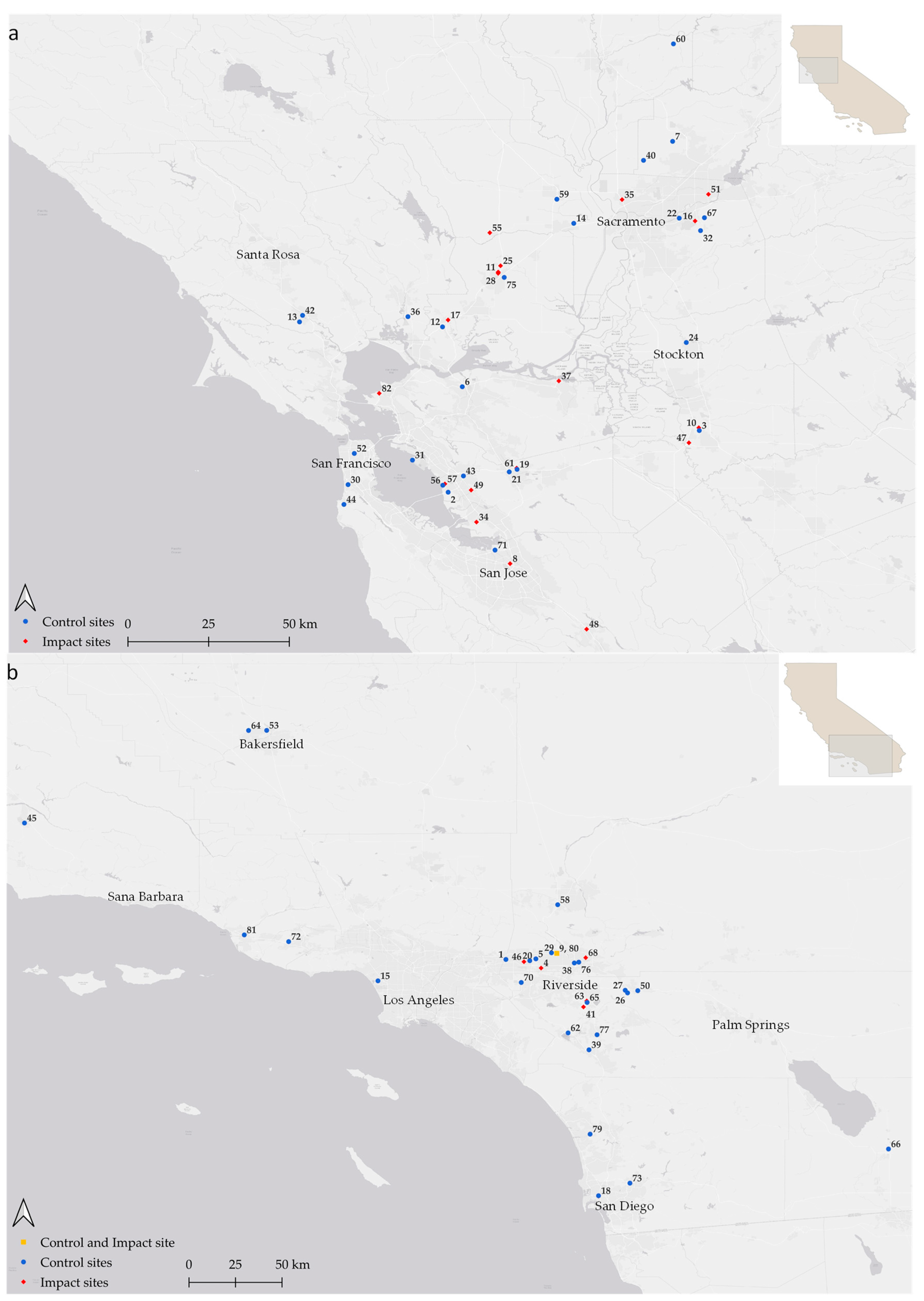
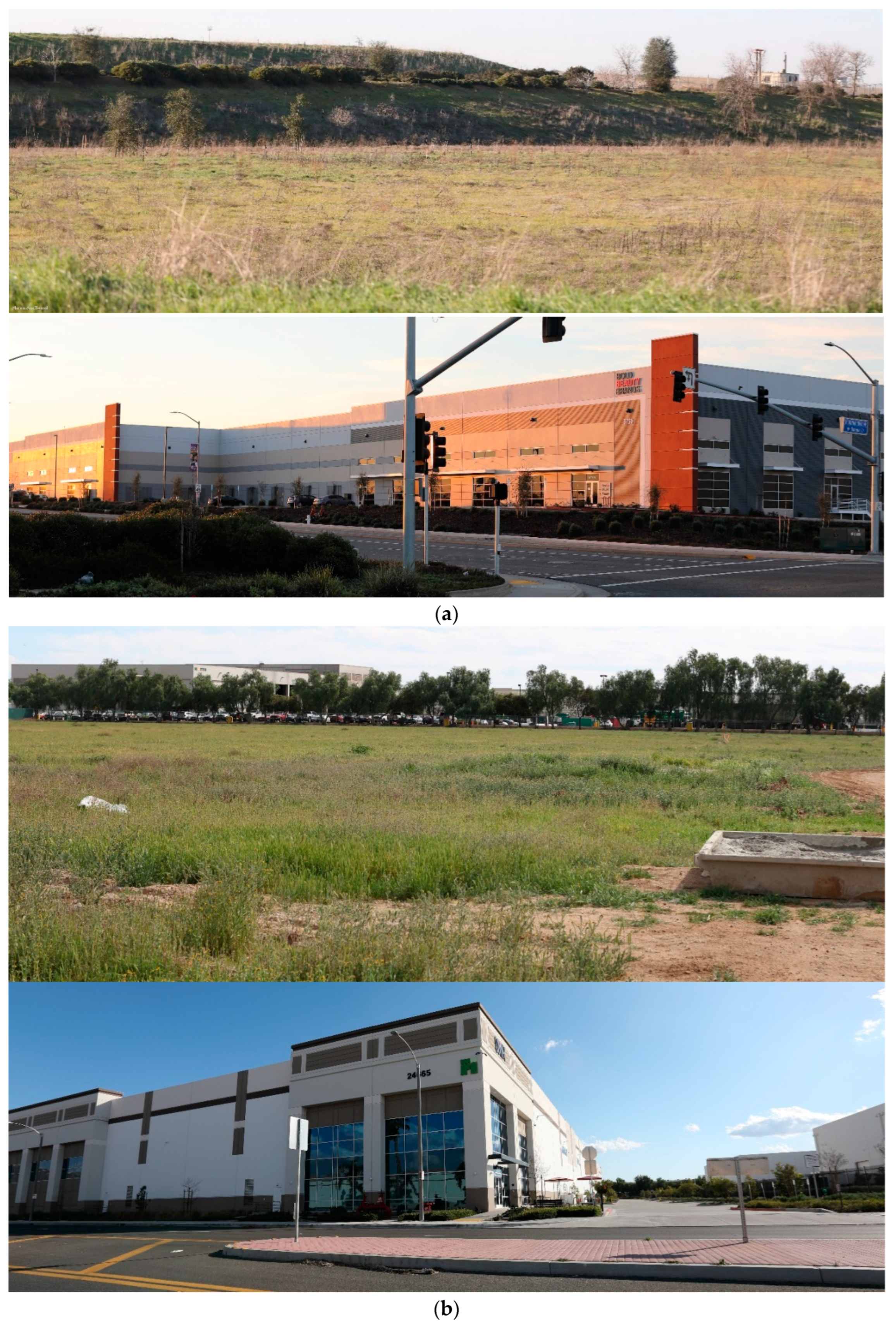
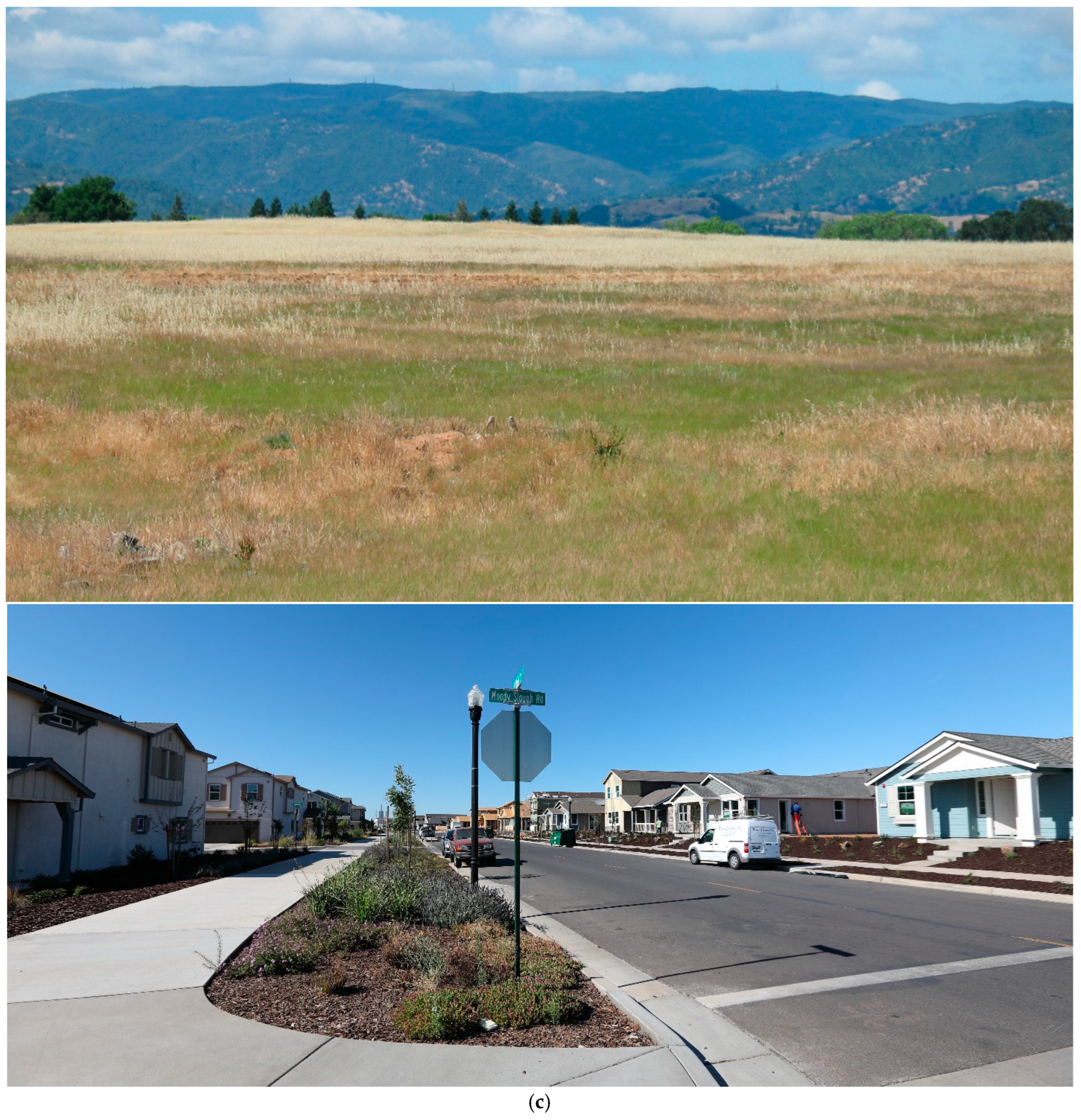
2.1. Study Area

Our study sites were clustered in the Sacramento and Central Valleys, the San Francisco Bay Area, and the coastal region of southern California (Figure 1). Each of these sites was selected because applications had been submitted for development. We later added follow-up surveys where practical and when we could closely match the date and start time of the initial surveys. Twenty-six of the sites had been developed by the time of our follow-up surveys, whereas fifty-two sites remained undeveloped. Developed sites were those for which the intended structures of the project were completely or nearly completely built, but they did not have to be occupied (some structures remained vacant for extended periods) (Figure 2). Thirty-five of the sites were within or peripheral to existing urban, commercial, or industrial areas, but thirty were located on agricultural or desert landscapes (Table A1). The condition of most of our study sites was poor to moderate at the times of our initial surveys, as most sites had been disturbed by mechanical clearing of vegetation (Figure 3), frequent fires, off-road vehicle use, invasive plant species composition (Figure 4), or by other forms of pollution, e.g., dumping of waste materials and mowing for weed abatement. Only four of the sites were surrounded on all sides by open space. Study sites ranged from 0.526 ha to 1,549 ha (mean = 91.26 ha, SD = 255.44 ha), with the two largest study sites consisting of natural reserves, which we used as control sites.

2.2. Reconnaissance Surveys

We performed what are referred to in California as reconnaissance surveys, also known as general biological surveys. We intentionally implemented the same methodology as used by environmental consultants when they perform reconnaissance surveys. In these surveys, all species are recorded if detected by visual or auditory means or by signs such as burrows, tracks, or scat. Wildlife recorded included birds, mammals, amphibians, and reptiles. We surveyed by walking the perimeter of the site, or by a stationary vantage point, where we scanned for wildlife with the use of binoculars. We recorded those animals that were onsite, i.e., within the boundary of the project site, and which we refer to hereafter as onsite. We also recorded animals in the project area, which included those onsite and those we judged were close enough to the project site to readily make use of it, which was usually ≤100 m from the site. In most surveys, we recorded the time within the survey when a new species was detected, whether the species was on the project site or in the surrounding area, and the approximate abundance of that species. We recorded temperature, wind, and sky conditions at the start and end of most surveys, and we recorded ground conditions at all sites at the time of each survey.

Reconnaissance surveys are unbound by time, but typically last between one and several hours. We stopped our initial survey at each project site once our species detection rate declined to about one new species per 20 or 30 min, similar to the rule advocated by Watson [33]. These lower detection rates typically coincided with the increasing heat of the day or oncoming darkness of the evening. In the cases of our second surveys to represent the after phase of the experiment, we stopped each survey at the time it took to record all of the species that had been recorded in each initial survey.

Beginning in January 2020, we began to resurvey sites of proposed building projects that we had originally surveyed during the same time of year and about the same time of day between 1 and 19 years earlier. In addition to starting the repeat survey as close to the original start time as possible, we surveyed for the same duration and using the same person, or both of us if we had originally surveyed together. Of the sites we resurveyed, 52 had remained undeveloped and 26 had been developed since our initial survey. Upon each repeat survey, we assigned sites that remained undeveloped to the control group, and sites that were since developed to the impact group. We applied the same survey standards between control and impact sites.

2.3. BACI Tests

We compared our survey outcomes in a BACI experimental design. One metric of the survey outcome was the total number of vertebrate species seen during the survey, including species seen in the project area but off the project site. A second metric was the total number of species seen only on the project site. A third metric was the number of vertebrate species detected solely offsite. A fourth metric was the number of species uniquely detected at a site in one phase relative to the other phase. A fifth metric was the total number of live animals counted during the survey (excluding fossorial mammals indicated by signs of burrow activity). A sixth metric was the number of sites at which a species or group of species was detected. For each metric, we quantified the expected outcome at impact sites (E_IA) relative to the before–after change in outcomes at the control site, and the effect of the development on the impact treatment level:

E_{I A} = (\frac{C A}{C B}) \times I B

E f f e c t = \frac{(I A - E_{I A})}{E_{I A}} \times 100 %,

where treatment levels were CB = control-before, CA = control-after, IB = impact-before, and IA = impact-after.

We compared rates of species detections with increasing time into the survey by the following experimental treatment groups: control-before (CB), control-after (CA), impact-before (IB), and impact-after (IA). To arrive at these comparisons, we fit a nonlinear least-squares regression model to the cumulative number of species detected, Y, as a function of the number of minutes, X, into each survey. The form of the model was

Y = \frac{1}{\frac{1}{a} + b \times {(X + 1)}^{- c}}

, where X represents minutes into the survey, and a, b, and c were best-fit coefficients. Since the surveys varied in duration, this modeling approach was also useful for minimizing the effect of survey duration on the metric, number of species detected. We did this by using each model to predict the number of species that would be detected after one hour. We chose 1 h because it was within the data range of all but 4 of the surveys we completed. We also projected the model to 5 h for comparison.

We used 2-factor analysis of variance with interest mostly in the significance of the interaction effect between the before–after time period (BA) and the control–impact treatment (CI) of each BACI experiment, as implemented by others [34,35]. We performed the tests on data collected from the project areas as well as those strictly from onsite. Except for our model-predicted number of species detected after one hour of surveying, we log₁₀-transformed count variables, such as the number of species detected and number of animals counted. We visually examined normal probability plots, and we performed Hartley’s F-max test for homogeneity of variance to determine whether our tests met the assumptions of ANOVA. The assumptions were met in nearly every test. To further assess the 2-factor ANOVA interaction effects, we calculated their statistical power.

2.4. Effects of Other Factors

From the BACI test of the number of vertebrate species detected, we saved ANOVA model residuals for exploring whether additional variation in the data could be explained by factors represented by other measured variables. We did the same for the BACI test of the model-predicted number of vertebrate species detected at 1 h. We regressed both sets of residuals on survey duration (minutes of survey common to both the before and after phases) to compare the degrees to which the effect of survey duration had been reduced, and hence to decide which set of residuals to use in exploration of the effects of other factors, such as landscape and site attributes. Our objective was to maximally control for the effect of survey duration when testing whether and how the number of vertebrate species detected related to project size (ha), latitude, number of years between the surveys in the before and after phases, the similarity index [36], and as described in the following paragraph, the intensity of pre-survey actions that would have suppressed wildlife, landscape settings such as whether the site was infill, redevelopment, or surrounded by open space, and the site disturbance rating. We note that whereas the similarity index was intended to measure the similarity of community composition of constituent species, its true measurement must also be of species detection probabilities attributable to the surveys.

We categorized an urban setting index for each site as 0 = largely non-urbanized, 1 = urban infill, and 2 = redevelopment. We rated the connectivity of project site borders to adjacent open space (including agriculture) as 0%, 10%, 25%, 50%, 75%, and 100%. We categorized sites as having undisturbed vegetation; evidence of disturbance over the last 5 years or so; ruderal; mowed; neglected by accumulation of trash, construction debris, waste soil or machine parts; neglected by cessation of irrigation; burned; disked; graded; construction ongoing, or constructed, as well as combinations of the foregoing categories. From these categories, we rated sites for the level of disturbance as: 1 = natural and biologically intact, with no more than small patches of non-native vegetation; 2 = mostly intact, with some native and some non-native vegetation, or all native with some past ground disturbance; 3 = modified (disked or highly disturbed) in the past but with a substantial extent of vegetation, such as patches of shrubs or scattered trees; 4 = landscaped parks or golf courses; 5 = agriculture, including orchards and vineyards; 6 = agriculture, including row crops; 7 = parking lot with mature shrubs or trees, and where buildings do not cover the entire site; 8 = highly modified with little vegetation remaining; 9 = compacted, pervious ground with no vegetation remaining; 10 = impervious ground with no vegetation remaining; 11 = constructed buildings. We further categorized site conditions to represent the intensity of actions that likely would have suppressed wildlife as: 0 = none evident, 1 = low (ruderal, cleared fire break), 2 = routine disturbance, 3 = moderate (mowed, neglected), 4 = earlier intense (near-recent grading, regrowth after disking), 5 = intense (cleared, disked, disked and neglected), and 6 = very intense (converted to crop, graded, constructed).

2.5. Species Characteristics

We compared the species detected among surveys to identify the frequency that each was found in the before and after phases and between the control and impact treatment levels. We further grouped species into classes, including amphibians, reptiles, mammals, birds, grassland birds, raptors, synanthropic birds, non-native species, and special-status species. The latter class was informed by legal protections afforded species by state and federal statutes and by designations assigned to species by state and federal wildlife agencies (species names, species groupings, and special-status species are listed in Table A2). We measured development impacts to these classes by the mean number of species within each that was detected per survey.

3. Results

Impact sites differed from control sites in several ways, including their average smaller size, lower elevation, and 94 km more northerly locations (Table 1). On average, impact sites were half to less than half connected to open space, as compared to control sites. Impact sites also ranked higher on the urban setting index, which meant they were more likely to be infill or redevelopment projects. Furthermore, impact sites rated higher for the level of disturbance, even prior to development, and they ranked higher on the intensity of actions resulting in suppression of wildlife occurrences, even prior to development (Table 1). On average, the survey duration was briefer on impact sites by nearly half an hour, and the time between the first and second surveys was longer by 1.3 years, but the average difference in start times was insubstantial.

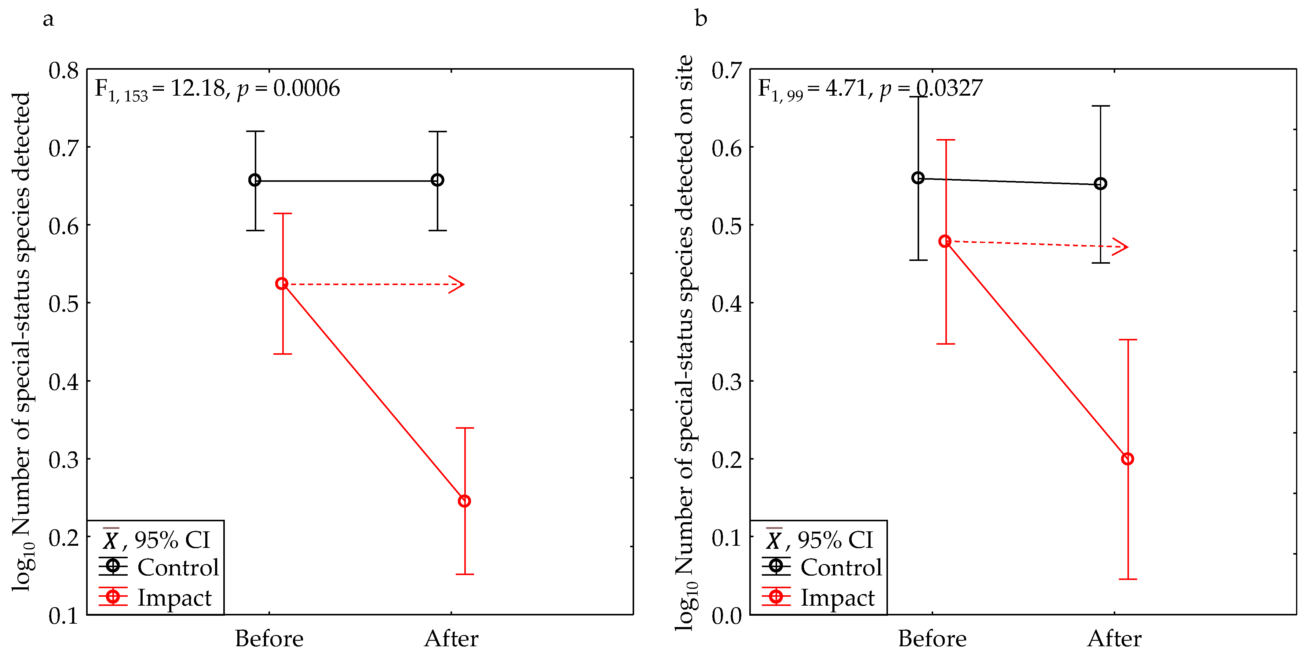
3.1. BACI Experiment

As part of our experiment, we completed 78 pairs of before and after surveys, or 156 surveys. Our cumulative number of species detections increased with the increasing survey duration, but the rates of these increases differed between sites in the control and impact treatment levels, and the mean rate was slowest among sites in the impact-after group, i.e., the sites that had been developed (Figure 5a). The model-predicted number of species detected by 1 h into a survey averaged about 10.4 in the IA group, as compared to 20.8 to 21.8 in the CB and CA groups. By 5 h, the disparity increased to 12.7 species detected in the IA group, as compared to 37.6 in the CB and CA groups (Figure 5b). At 1 h, the model-predicted number of species detected was 51% lower in the IA group, but at 5 h it was 66% lower.

We observed large changes in species composition and relative abundance among the project sites that were developed before our second survey. Some of the species we detected in the before phase were relatively abundant, but their abundance sharply declined after development. For example, at the CenterPoint Warehouse Project site in Manteca, our before and after counts changed from 300 to 9 American crows, from 40 to 3 mourning doves, from 400 to 0 western meadowlarks, and from 30 to 0 house finches. On average, we counted 88% fewer vertebrate animals, including 85% fewer animals of special-status species, on impact sites after development, and we detected 44% fewer vertebrate species on impact sites after development, and 62% fewer vertebrate species on the project footprint (Table 2).

We also observed changes in species composition and relative abundance among the project sites that did not undergo development and which we treated as our control sites. For example, at the Operon HKI Project site in Perris, our before and after counts shifted from 10 to 20 savannah sparrows (Figure 6), 0 to 20 western meadowlarks, and 0 to 20 horned larks. On average, we detected about 2–3 additional species in most groups of species during our second surveys among the control sites, and we counted about 26% more birds, but notably we counted 56% fewer species, and 44% fewer animals of special-status species vertebrate wildlife (Table 2).

In the before phase, the number of species detected averaged fewer at the impact sites compared to the controls, whereas the number of animals counted averaged more at the impact sites compared to the controls (Table 2). Consequently, the control–impact main effects were significant for all but one of the metrics consisting of the number of species detected, whereas they were not significant for any of the metrics of the number of animals counted (Table 3). The before–after main effects were significant for the number of vertebrate species detected and the number of birds detected, but not for the numbers of species detected of mammals or reptiles and amphibians. The before–after main effects were significant for all the metrics of the number of animals counted. However, whereas these main effects point towards potential biases, our main interest was in the interaction effect, which informs of the impact of the action (development), and which presumably would have been largely controlled for in the experiment.

After development, the average number of vertebrate wildlife species we detected declined by 48% within the project area, and by 66% within the bounds of the project sites (Table 2, Figure 7a,b). These declines were significant (Table 3). At the same time, the number of vertebrate wildlife species we detected solely offsite increased by 334% (Table 2, Figure 7c), which was significant (Table 3).

The average number of bird species declined by 45% within the project area, and by 64% within the bounds of the project sites (Table 2). These declines were also significant (Table 3). Although not significant due to insufficient statistical power (Table 3), the average number of mammal species declined by 79% across the entire viewshed and by 92% within the bounds of the project sites, and the average number of amphibians and reptiles (“herps”) declined by 47% in the project area, and by 100% within the bounds of the project sites (Table 2).

After development, the average number of vertebrate animals we counted declined by 90% within the project area (Figure 8a), and by 89% within the bounds of the project sites (Table 2). These declines were significant (Table 3). The average number of birds we counted declined by 91% within the project area (Table 2, Figure 8b), and by 89% within the bounds of the project sites (Table 2), both of which were significant (Table 3).

After development, the average number of special-status species declined by 49% within the project area, and by 58% within the bounds of the project sites (Table 2, Figure 9a). The average number of vertebrate animals of special-status species that we counted declined by 70% within the project area, and by 82% within the bounds of the project sites (Table 2, Figure 9b). All of these declines were significant (Table 3).

After development, the average model-predicted number of vertebrate species detected in one hour of surveying declined by 37% within the project area (Table 2, Figure 10a), which was significant (Table 3). The number of vertebrate species uniquely detected at a site in one phase relative to the other phase declined by 74% (Table 2, Figure 10b), which was also significant (Table 3).

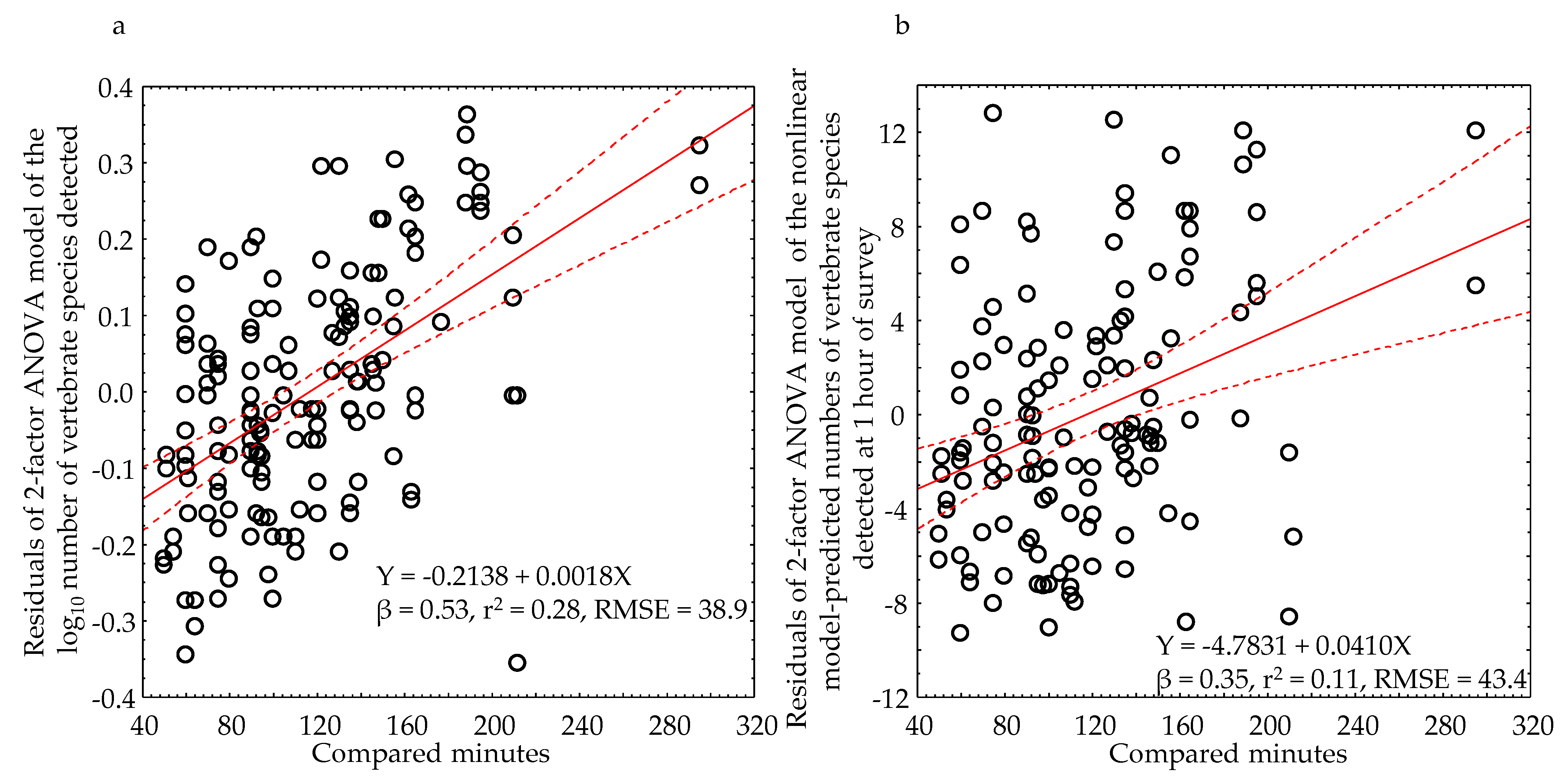
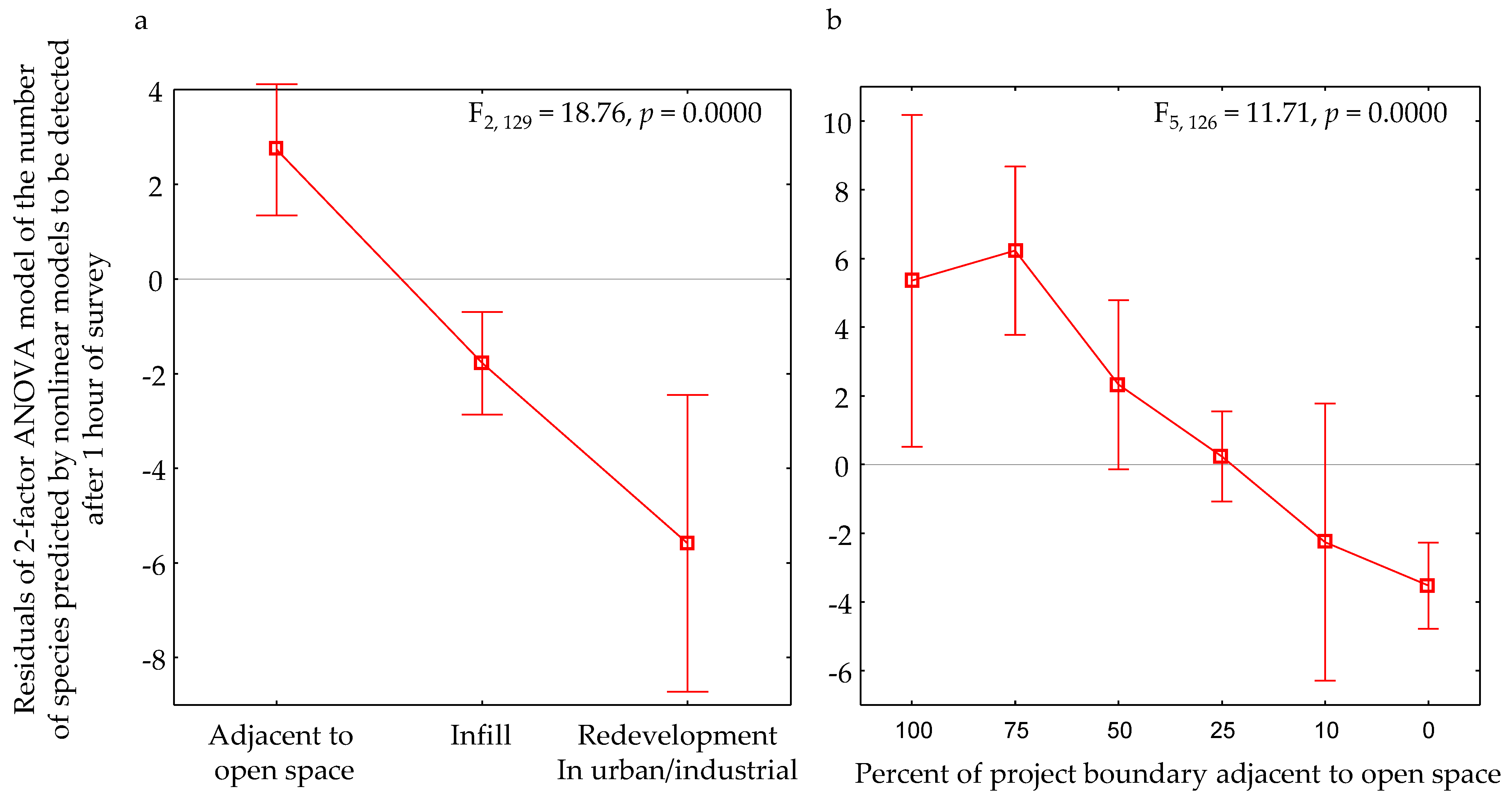
3.2. Effects of Other Factors

We found that the ANOVA model residuals significantly increased with the increasing survey duration (Figure 11a), which should have had no effect on our BACI tests, but which would likely confound our tests for the effects of other factors. Therefore, we used the ANOVA residuals from the BACI experiment involving model-predicted numbers of vertebrate species detected after one hour of surveying, assuming the residuals from this test would most effectively minimize any residual variation of survey duration. The model-derived residuals continued to increase with the increasing survey duration (Figure 11b), but with a much smaller r², a smaller standardized slope coefficient, β, and a slightly larger root-mean squared error (RMSE), all of which indicated a reduced residual effect of survey duration.

Model-adjusted residuals related only weakly with multiple variables, including with the intensity of pre-survey actions that would have suppressed wildlife (F_6,125 = 1.14, p = 0.3437), project size (ha), latitude, the number of years between the surveys in the before and after phases, the site disturbance rating, and the similarity index measured between the before and after surveys at the same site. However, they significantly differed among groups of sites located in open space or in an infill setting, or as redevelopment within developed areas such as cities (Figure 12a). Mean residuals were positive within open areas, and negative in areas of infill or redevelopment. Model-adjusted residuals also significantly differed by levels of connectedness to open space (Figure 12b). Mean residuals were positive among sites with >50% connectivity to open space, and negative among sites with <50% connectivity to open space.

3.3. Species Characteristics

A few species of wildlife increased in the frequency of detection among project sites that were developed, including, in order of increase: Cooper’s hawk, ruby-crowned kinglet, yellow-rumped warbler, California gull, black phoebe, house cat, and Anna’s hummingbird (Table A2). Many more species, however, decreased in the frequency of detection, including, in order of decrease: California ground squirrel, Botta’s pocket gopher, burrowing owl, California quail, California vole, Cassin’s kingbird, cedar waxwing, coyote, great-tailed grackle, killdeer, loggerhead shrike, northern rough-winged swallow, oak titmouse, orange-crowned warbler, Sierran treefrog, white-tailed kite, white-throated swift, and yellow-billed magpie, followed by: western meadowlark, red-winged blackbird, western fence lizard, great egret, American robin, eastern gray squirrel, mallard, American kestrel, red-tailed hawk, white-crowned sparrow, black-tailed jackrabbit, dark-eyed junco, western gull, savannah sparrow, European starling, California towhee, bushtit, lesser goldfinch, Brewer’s blackbird, Canada goose, northern flicker, turkey vulture, Nuttall’s woodpecker, barn swallow, western kingbird, Swainson’s hawk, rock pigeon, mourning dove, red-shouldered hawk, double-crested cormorant, house finch, Eurasian collared-dove, California scrub-jay, cliff swallow, house sparrow, desert cottontail, northern mockingbird, common raven, American goldfinch, Say’s phoebe, and American crow (Table A2).

Groups of wildlife that declined the most following development included, in the following order: amphibians, mammals, grassland birds, raptors, special-status species, all birds as a group, non-native birds, and synanthropic birds (Table 4).

4. Discussion

4.1. Effects of Development on Vertebrate Wildlife

Assuming our sampling design sufficiently controlled for differences in size, condition, and setting between control and impact sites, and for differences in survey duration, our experiment revealed substantial reductions in vertebrate species richness and numerical abundance caused by development. Although our surveys likely failed to detect all the species or to count all the animals available at the times of our surveys, we believe it is unlikely that underlying survey biases could have substantially confounded the magnitudes of development impacts we measured. We suggest, for example, that survey bias cannot explain the 74% decline we measured in the number of vertebrate species that we uniquely detected at a site in one phase relative to the species we detected in the other phase. The magnitude of this effect was too large to be explained by anything other than a profound shift in the species composition of project sites following development. Site-specific project impacts are generally devastating to wildlife.

Immediately offsite, we detected a >3-fold increase in the number of vertebrate species that were solely offsite. This increase likely reflected a spatial shift by a few species in response to development, but the numbers of species we detected solely offsite were small regardless of the treatment group. Many of the species we detected on project sites were also detected offsite, but we did not record which species were both on- and off-site until the last few surveys.

Only seven species of wildlife increased in the frequency of detection among surveys at sites where development preceded our surveys in the after phase of our experiment. Of these seven species, two were generalists—California gull and yellow-rumped warbler—consistent with the finding that generalist species of birds were most often the species that adapt to urbanized landscapes [37]. Black phoebe, house cat, and Anna’s hummingbird were three other species that increased in the frequency of occurrence, but their increases were small. Ruby-crowned kinglet’s increase remains questionable, considering the small sample sizes, but Cooper’s hawk is a specialized forager that appears to capitalize on urbanization. Otherwise, majority of wildlife species with sufficient sample sizes declined in their numbers of detection among our surveys at sites where buildings were constructed in the period between our before and after surveys. We suggest that the categorization of wildlife as urban avoiders, urban adapters, and urban exploiters [38] provides a useful framework for understanding how wildlife respond to urbanization, but we also suggest that most of the urban adapters and urban exploiters can be vulnerable to the final stage of development at a given site.

Whereas invasive and synanthropic species might fare better than native species in urban environments [39], we found that species in both these groups also declined after the development of project sites, similar to the finding of Scott [31]. The declines of species in these groups were not as great as for raptors and grassland bird species, but they were nevertheless substantial. Overall, the development projects reduced the species richness and wildlife abundance.

Terrestrial vertebrate species declined the most in our study, consistent with previous findings [40,41,42], but the declines we measured were not significant due to insufficient statistical power. Though not statistically significant, we suggest that our measured declines ought to be considered biologically significant. In the field, finding fewer or no terrestrial mammals and amphibians where we had seen them before was noticeable, and we assert that these declines resulted directly from development. Some of these terrestrial vertebrate species were ecological keystone species, such as the Botta’s pocket gopher (Figure 13) and California ground squirrel. The California ground squirrel, in particular, has been found to limit the distribution of multiple special-status species, such as the burrowing owl [43] and loggerhead shrike [44]. Indeed, where development preceded our second surveys, California ground squirrels were not observed, and neither were any of the burrowing owls or loggerhead shrikes that we had seen at those sites prior to development (Figure 13).

4.2. Landscape Effects

Andrén [45] predicted that “landscapes with highly fragmented habitat, patch size and isolation will complement the effect of habitat loss and the loss of species or decline in population size will be greater than expected from habitat loss alone”. Our results tended to support this prediction. Our mean ANOVA residuals of the number of vertebrate species detected at one hour of surveying was negative among sites in urban infill and redevelopment settings, and positive among sites surrounded by open space (Figure 12), meaning there were relatively fewer species in urban settings and relatively more in settings of open space. This result resembles that of another study that found that bird species richness in urban settings correlated positively with bird species richness in adjacent landscapes composed of managed or natural vegetation [46].

We note, also, that we detected more species composed of smaller average counts of individuals in the before phase of control sites, as compared to the before phase of impact sites—the sites that were to be developed later during our study; alternatively, we found smaller numbers of species of larger average counts at impact sites even in the before phase, which was a pattern previously noted [31]. By the time we initiated our first surveys at the impact sites, they were already different in species composition. In fact, the impact sites differed from control sites with their average smaller size and lower elevation, but perhaps more importantly, with their lower connectivity to open space, their higher average rank on the urban setting index, their higher average ratings for the level of disturbance, and their average higher intensity of actions resulting in suppression of wildlife occurrences. We also surveyed impact sites more briefly than we surveyed control sites, but our briefer surveys probably reflected the smaller average size of impact sites. Earlier in our study, we could not have predicted which sites would be developed sooner than other sites, but now it appears that smaller infill sites tend to be managed more aggressively to suppress wildlife, tend to support fewer species, and are more likely to be approved for development.

Numerous species of vertebrate wildlife were found only at control sites, further revealing the potential wildlife community difference that already existed by the time of our first surveys at project sites, but which also prevented species-specific measures of development effects. Such species included Allen’s hummingbird and the black-chinned hummingbird, American coot, black-necked stilt, blue-gray gnatcatcher and California gnatcatcher, bobcat, California thrasher, common yellowthroat, great horned owl, hairy woodpecker, hooded oriole, horned lark, marsh wren, mule deer, olive-sided flycatcher, ring-billed gull, song sparrow, striped skunk, western bluebird, white-breasted nuthatch, and Wilson’s warbler. A mitigating factor in our findings of these species only at control sites was the fact that we surveyed twice the number of control sites compared to impact sites.

4.3. Evidence of Ongoing Cumulative Effects of Urbanization

Before- and after-phase surveys at control sites revealed a trend that was likely more indicative of cumulative effects at landscape scales, as these surveys were of equal number and free of onsite development. Despite our average detections of about 2–3 additional species after our second surveys at control sites, and despite our average counts of 26% more birds in the absence of site-specific development, in our follow-up surveys we detected 56% fewer special-status species, and we counted 44% fewer animals of special-status species. During our study, special-status species of vertebrate wildlife appeared to have been on the decline within the regions of our study. These declines indicate that project-specific mitigation measures have been failing to avoid cumulative impacts.

4.4. Potential Biases

We endeavored to design and implement our study to minimize the effects of bias and error by standardizing site-specific survey dates, start times, survey duration, and survey methods. Where we walked a transect along the perimeter of a site during the first survey, we tried to repeat the walk of the same transect during the second survey. We surveyed most sites the second time with the same investigator, or both of us, as we had surveyed the first time. However, there was variation in the survey methods between sites, most notably the survey duration. We attempted to adjust our survey findings for variation in the survey duration by best-fitting a nonlinear model to each survey’s increase in the cumulative number of detected species with the increasing time into the survey. From each model, we predicted the number of species detected after one hour of surveying, which was enough time to predict a substantial number of species but also well within the range of survey durations that we completed among the project sites. Nevertheless, the ANOVA model’s residuals derived from model-predicted numbers of species detected after 1 h continued to weakly increase with the increasing survey duration among project sites (Figure 11b). We did not eliminate the effects of survey duration. We do not believe that the remaining effect of survey duration significantly affected our study results, but we note this effect for designing future studies of the effects of urbanization on wildlife. The effect was stronger without the model-based adjustments, but the model-based adjustments appear to have been sample-dependent. The duration of the survey affects the pattern of the increasing cumulative number of species with the increasing survey duration, and hence affects the nonlinear model fit to the pattern. It might be possible to standardize the pattern in the cumulative number of species detected by standardizing Watson’s [33] results-based stopping rule, or by standardizing the survey duration [47]. If the latter, then we recommend a relatively long survey duration, such as ≥2 h.

Another potential bias is the change in detection rates of wildlife species after the project sites were developed. Our probability of detecting the average bird was likely higher after the available perches transitioned from trees and shrubs to light standards on parking lots and the rooflines of warehouses. The detection likelihood might have increased after opportunities to view flying birds transitioned from views of complex environmental backgrounds to the walls of warehouses, although the environmental backgrounds of most of our project sites were rather simple. At some sites, the landscaping around warehouses and other new structures comprising the project might have been simpler than the pre-construction environments, thus better enabling us to detect an animal on those portions of the project site had the animals been present. Although we acknowledge this potential bias, the amount of survey time we committed to each site gave us ample opportunity to detect the species of wildlife that were truly there at the times of both of our surveys. At developed sites, our rates of detection of wildlife species were much slower (Figure 8) and the total numbers of species detected were fewer (Table 2 and Table 3), but we believe that these differences more likely reflected biological conditions than they did our survey detection rates.

Another potential bias was the differential detection rates among species of wildlife. We likely disproportionately detected the most readily detectable species, while failing to detect those species that are smallest in body size, nocturnal, fossorial, and more cryptic. Furthermore, the numerical abundances we attributed to the species we detected likely often differed from the true numerical abundances, even within the spatial and temporal scopes of our surveys. Whereas our counts of animals might have more often approached the true numbers of the largest-bodied species, such as red-tailed hawks (Buteo jamaicensis) and mule deer (Odocoileus hemionus), they likely under-represented the smaller-bodied species, such as sparrows, warblers, western fence lizards, and Belding’s orange-throated whiptails.

Our baseline settings in the before-phase surveys were far from pristine at most project sites, but they nevertheless served as baselines for measuring changes brought about by construction of buildings to the number of vertebrate species detected and to our counts of live animals, which we intended to indicate, respectively, as species richness and relative abundance. We use the term “indicate” here because we recognize that we did not truly measure species richness nor true abundance, as multiple potential biases and errors prevented such measurement [48]. On the other hand, our surveys were of sufficient duration to detect most of the diurnal bird species that would have been available to us at each site at the times of our surveys [47].

5. Conclusions

By use of an experiment including control sites, we found that development projects directly and substantially reduced vertebrate wildlife species richness and wildlife abundance. Vertebrate wildlife species most affected by development in California were terrestrial species, as well as grassland birds, raptors, and special-status species. We also found that special-status species declined on control sites even in the absence of site-specific development, which indicates widespread ineffectiveness of project-level mitigation measures, and hence cumulative impacts from regionwide urbanization. More needs to be learned as soon as possible about the impacts of urbanization on wildlife. Experiments need to be designed with the use of control sites to more directly measure project-level effects, and with sampling plots to monitor regional effects of urbanization.

To follow-up on Marzluff’s [18] recommendation, and to take advantage of the opportunities to measure the effects of development projects on wildlife, the California Environmental Quality Act should be amended to require that reconnaissance surveys be repeated in each season of the year preceding the public circulation of an environmental review document. The required mitigation plan should include funding for post-construction reconnaissance surveys of the same methods, number, and seasonal spacing to more robustly represent the wildlife community before and after development. The CEQA should be further amended to require a sufficient funding allocation from each project applicant that would be directed to control sites, which should also be integrated into cumulative effects monitoring. Whereas the CEQA requires a cumulative impacts analysis, data needed to analyze the cumulative impacts to wildlife usually do not exist, and thus consultants’ analyses of cumulative impacts are speculative. Since long-term monitoring is often not required, and thus not performed, the consultants’ conclusions about the cumulative impacts cannot be confirmed nor denied. Long-term monitoring would give all parties involved a better understanding of how to analyze the cumulative impacts, because we would have a better understanding of how development truly affects each species. A cumulative impacts fund should be administered by a trusted party to ensure that unbiased, qualified biologists implement long-term monitoring of wildlife within a spatial area that can meaningfully inform of cumulative effects.

To soften the impacts of urbanization on wildlife, the CEQA should be amended to require the use of native and xeric-adapted plants in landscaping, i.e., chaparral, grassland, and locally appropriate scrub plants, as opposed to landscaping with lawn and exotic shrubs. Native plants offer more structure, cover, food resources, and breeding substrates for wildlife than landscaping with lawn [49,50] and increase the abundance and diversity of birds, especially native birds [51,52,53,54]. Landscaping with native plants is a way to interconnect patches of habitat for wildlife [55,56].

The CEQA should also be amended to require project applicants to contribute funding to wildlife rehabilitation facilities. As projects are built, and wildlife are subsequently injured by the windows of buildings, project-generated traffic, and free-ranging house cats of new residents, wildlife rehabilitation facilities should be provided the resources they need to attempt to rectify these types of project impacts.

Author Contributions

Conceptualization, K.S.S.; methodology, K.S.S. and N.L.S.; formal analysis, K.S.S.; investigation, K.S.S. and N.L.S.; writing—original draft, K.S.S. and N.L.S.; writing—review and editing, N.L.S.; supervision, K.S.S. All authors have read and agreed to the published version of the manuscript.

Funding

The research specific to this study received no external funding, but all the surveys in the before phase of the experiment were funded by the authors’ clients who had interests in the outcomes of the proposed projects. All but one of the surveys in the after phase were self-funded.

Data Availability Statement

Data supporting the reported results can be requested from the authors.

Acknowledgments

We thank our clients for funding the initial survey at each site of the proposed development projects. We also thank the two anonymous peer reviewers for their very helpful reviews of earlier drafts of this manuscript.

Conflicts of Interest

We declare no conflict of interest.

Appendix A

Table A1. Project site and survey attributes.

Pair	Treatment Level	Phase	Survey Minutes Compared	Project	Location	Proposed Use	Survey Date	Start Time	Ha	Conditions on the Ground
1	Control	Before	64	11th Street Development	Upland	Warehouse	8 November 2020	6:40	1.98	Ruderal scrub around old cement pad
1	Control	After	64	11th Street Development	Upland	Warehouse	24 November 2021	6:43	1.98	Same as above
2	Control	Before	135	4150 Point Eden Way Industrial Development	Hayward	Warehouse	11 May 2021	6:40	4.37	Grassland bounded by salt ponds, including those of Eden Landing Reserve, CA Highway 92, and industrial warehouses
2	Control	After	135	4150 Point Eden Way Industrial Development	Hayward	Warehouse	10 May 2022	7:12	4.37	Same as above
3	Control	Before	135	Airport Business Centre	Manteca	Warehouse	28 April 2021	16:17	9.51	Mowed hay bordered on the north by warehouses
3	Control	After	135	Airport Business Centre	Manteca	Warehouse	28 March 2022	16:31	9.51	Unmowed hay bordered on the north and west by warehouses
4	Impact	Before	50	Almond Street Warehouse	Fontana	Warehouse	27 April 2019	9:25	4.05	Former parking lot with ornamental trees
4	Impact	After	50	Almond Street Warehouse	Fontana	Warehouse	25 April 2022	8:50	4.05	Warehouse
5	Control	Before	105	Alta Cuvee	Rancho Cucamonga	Residential	4 September 2021	6:54	2.55	Highly disturbed dirt field with low shrubs and non-native grass
5	Control	After	105	Alta Cuvee	Rancho Cucamonga	Residential	30 August 2022	7:04	2.55	Same as above
6	Control	Before	163	Amare Apartments	Martinez	Residential	4 June 2018	17:17	2.45	Disked woodland savannah
6	Control	After	163	Amare Apartments	Martinez	Residential	19 July 2021	17:07	2.45	Same as above
7	Control	Before	130	Antonio Mountain Ranch	Placer County	Residential	18 November 2002	14:30	359.00	Grassland/vernal pool complex with riparian
7	Control	After	130	Antonio Mountain Ranch	Placer County	Residential	16 November 2021	14:45	359.00	Same as above
8	Impact	Before	135	Brokaw Campus	San Jose	Corporate Campus	16 November 2018	12:45	6.78	Disked with ruderal cover
8	Impact	After	135	Brokaw Campus	San Jose	Corporate Campus	30 October 2021	12:42	6.78	Four tall buildings
9	Control	Before	80	Casmalia and Linden	Rialto	Warehouse	21 June 2020	6:10	2.77	Grassland and shrubs
9 ^a	Control	After	80	Casmalia and Linden	Rialto	Warehouse	31 July 2021	6:12	2.77	Grassland and shrubs
10	Impact	Before	94	CenterPoint	Manteca	Warehouse	31 October 2018	16:15	9.12	Ruderal vegetation subsequent to grading
10	Impact	After	94	CenterPoint	Manteca	Warehouse	11 November 2021	15:26	9.12	Warehouse with parking lot
11	Impact	Before	100	Cessna and Aviator Warehouse	Vacaville	Warehouse	12 August 2018	18:00	5.21	Disked annual grassland
11	Impact	After	100	Cessna and Aviator Warehouse	Vacaville	Warehouse	31 August 2022	18:07	5.21	Warehouse and parking lot
12	Control	Before	95	Cordelia Industrial	Cordelia	Warehouse	16 October 2019	15:54	13.11	Disked annual grassland with some regrowth next to riparian
12	Control	After	95	Cordelia Industrial	Cordelia	Warehouse	7 October 2021	12:38	13.11	Disked annual grassland next to riparian; new houses on west side
13	Control	Before	165	Davidon Homes	Petaluma	Residential	11 February 2021	7:41	23.74	Grassland and riparian oak woodland
13	Control	After	165	Davidon Homes	Petaluma	Residential	1 March 2022	7:33	23.74	Same as above
14	Control	Before	54	Aggie Research Campus	Davis	Residential	13 April 2020	18:39	74.90	Planted sugarbeets, wheat, almonds
14	Control	After	54	Aggie Research Campus	Davis	Residential	2 April 2022	18:33	74.90	Wheat, dirt furrows, planted sugarbeets
15	Control	Before	93	Del Rey Pointe Residential Project	Playa Del Rey	Residential	31 October 2019	14:07	1.16	Ruderal vegetation bordered by Eucalyptus and 3 concrete-lined streams
15	Control	After	93	Del Rey Pointe Residential Project	Playa Del Rey	Residential	18 October 2021	13:54	1.16	Ruderal vegetation undergoing clearing by tractor; bordered by Eucalyptus and 3 concrete-lined streams
16	Impact	Before	122	GLP Store	Mather	Warehouse	12 February 2020	6:56	3.76	Annual grassland
16	Impact	After	122	GLP Store	Mather	Warehouse	18 February 2022	7:09	3.76	Warehouse
17	Impact	Before	90	Green Valley II	Fairfield	Residential	18 November 2019	9:00	5.39	Disked grassland with 1 oak and bordered by shrubs
17	Impact	After	90	Green Valley II	Fairfield	Residential	7 December 2021	9:47	5.39	Nearly built warehouse and apartments
18	Control	Before	120	Hillcrest LRDP	Bachman Canyon	None	9 November 2019	7:00	12.95	Diegan coastal sage scrub
18	Control	After	120	Hillcrest LRDP	Bachman Canyon	None	11 December 2021	7:11	12.95	Same as above
19	Control	Before	90	IKEA Outlet	Dublin	Warehouse retail	26 March 2018	11:15	11.11	Ruderal and annual grassland
19	Control	After	90	IKEA Outlet	Dublin	Warehouse retail	25 March 2022	9:53	11.11	Ruderal and annual grassland; tractors and trucks onsite, and about 15% to 20% is graded
20	Control	Before	110	Jersey Industrial Complex	Rancho Cucamonga	Warehouse	16 June 2021	6:26	2.99	Ruderal vegetation on disturbed soil, surrounded by warehouses and major roads and railroad tracks
20	Control	After	110	Jersey Industrial Complex	Rancho Cucamonga	Warehouse	11 July 2022	6:30	2.99	Previously disked, non-native grass present, surrounded by warehouses and major roads and railroad tracks
21	Control	Before	120	Johnson Drive Economic Zone	Pleasanton	Warehouse retail, hotel	29 July 2019	17:38	16.19	Mix of developed structures, vacant lots, and grassland
21	Control	After	120	Johnson Drive Economic Zone	Pleasanton	Warehouse retail, hotel	26 July 2021	17:46	16.19	Same as above
22	Control	Before	195	Kassis	Rancho Cordova	Residential	3 December 2020	7:47	16.51	Disked grassland and abandoned walnuts
22	Control	After	195	Kassis	Rancho Cordova	Residential	2 November 2021	7:39	16.51	Same as above
24	Control	Before	70	Lake Home	Lodi	Residential	13 March 2019	8:28	3.56	Abandoned orchard
24	Control	After	70	Lake Home	Lodi	Residential	25 March 2022	7:26	3.56	Same as above
25	Impact	Before	92	LDK Warehouse	Vacaville	Warehouse	10 November 2018	7:50	27.88	Disked annual grassland, riparian
25	Impact	After	92	LDK Warehouse	Vacaville	Warehouse	13 November 2021	7:53	27.88	Operational warehouse and nearly completed empty warehouse
26	Control	Before	127	Legacy Highlands	Beaumont, upper	Residential	4 May 2021	17:39	647.50	Sage scrub
26	Control	After	127	Legacy Highlands	Beaumont, upper	Residential	24 April 2022	17:34	647.50	Sage scrub
27	Control	Before	189	Legacy Highlands	Beaumont, lower	Residential	5 May 2021	6:02	647.50	Riparian, grassland, sage scrub
27	Control	After	189	Legacy Highlands	Beaumont, lower	Residential	26 April 2022	6:02	647.50	Riparian, grassland, sage scrub
28	Impact	Before	90	Logisticenter at Vacaville	Vacaville	Warehouse	1 September 2018	7:50	5.68	Disked annual grassland
28	Impact	After	90	Logisticenter at Vacaville	Vacaville	Warehouse	5 September 2021	7:48	5.68	Warehouse surrounded by warehouses on 3 sides, disked on 4th side
29	Control	Before	100	Mango Avenue	Fontana	Warehouse	24 January 2021	7:33	2.35	Ruderal grassland
29	Control	After	100	Mango Avenue	Fontana	Warehouse	13 February 2022	7:25	2.35	Ruderal grassland
30	Control	Before	112	Vista Mar	Pacifica	Residential	20 August 2020	6:59	0.53	Trees, shrubs, grassland
30	Control	After	112	Vista Mar	Pacifica	Residential	15 September 2021	7:17	0.53	Trees, shrubs, grassland
31	Control	Before	75	Marriott Hotel	Harbor Bay Parkway, Alameda	Hotel	16 November 2018	15:18	2.23	Ruderal cover on disked field lined by trees
31	Control	After	75	Marriott Hotel	Harbor Bay Parkway, Alameda	Hotel	30 October 2021	14:54	2.23	Same as above
32	Control	Before	188	Mather South Masterplan	Mather	Residential	16 February 2019	8:02	343.17	Annual grassland, wetland, riparian
32	Control	After	188	Mather South Masterplan	Mather	Residential	6 February 2022	7:20	343.17	Same as above
33	Impact	Before	145	Monte Vista Warehouse	Vacaville	Warehouse	23 June 2019	6:48	4.67	Disked grassland with volunteer shrubs/trees
33	Impact	After	145	Monte Vista Warehouse	Vacaville	Warehouse	16 June 2021	6:48	4.67	Nearly completely constructed warehouse; field to west under construction wtih pad
34	Impact	Before	70	Morton Salt Plant	Newark	Warehouse	8 May 2018	16:58	12.10	Abandoned salt ponds
34	Impact	After	70	Morton Salt Plant	Newark	Warehouse	3 June 2021	16:20	12.10	Warehouses next to row of Eucalyptus
35	Impact	Before	75	Natomas Crossing	Natomas	Commercial	30 June 2018	19:00	27.60	Feral grassland on disked soil
35	Impact	After	75	Natomas Crossing	Natomas	Commercial	9 June 2021	18:30	27.60	New buildings and parking lots; field to east was disked
36	Control	Before	90	Nova Business Park	Napa	Warehouse	15 July 2018	18:50	9.39	Annual grassland and riparian forest
36	Control	After	90	Nova Business Park	Napa	Warehouse	14 July 2021	18:19	9.39	Annual grassland and riparian forest, but early grading for project over past month or two and lots of development in surrounding area
37	Impact	Before	70	Oakley Logistics Center	Oakley	Warehouse	22 November 2019	8:04	152.04	Marsh, grassland, riparian, disturbed
37	Impact	After	70	Oakley Logistics Center	Oakley	Warehouse	7 December 2021	7:55	152.04	Warehouses and parking lots
38	Control	Before	90	Olympic Holding Inland Center	San Bernardino	Warehouse	1 December 2019	8:18	2.12	Barren ground and ruderal vegetation lined by trees
38 ^b	Control	After	90	Olympic Holding Inland Center	San Bernardino	Warehouse	6 December 2021	8:24	2.12	Barren ground and ruderal vegetation lined by trees
39	Control	Before	75	PARS Global Storage	Murietta	Warehouse	31 October 2019	10:06	1.28	Shrubs, grass, trees
39	Control	After	75	PARS Global Storage	Murietta	Warehouse	19 October 2021	10:02	1.28	Shrubs, grass, trees
40	Control	Before	177	Regional University	Roseville	University	15 January 2008 ^a	16:10	468.42	Annual grasslands, vernal pools
40 ^c	Control	After	165	Regional University	Roseville	University	12 January 2022 ^a	15:13	468.42	Annual grasslands, vernal pools
41	Impact	Before	150	Rider Warehouse	Perris	Warehouse	22 July 2019	6:55	3.89	Disked annual grassland
41 ^d	Impact	After	150	Rider Warehouse	Perris	Warehouse	28 March 2021	6:50	3.89	Warehouse
42	Control	Before	138	Clover Project	Petaluma	Residential	13 July 2020	17:24	1.36	Grassland with a few mature trees, next to Petaluma River
42	Control	After	138	Clover Project	Petaluma	Residential	22 July 2021	17:30	1.36	Grassland with a few mature trees, next to Petaluma River
43	Control	Before	135	Ruby Street	Castro Valley	Multi-family housing	17 October 2020	7:23	2.55	Grass meadow next to riparian forest of San Lorenzo Creek and otherwise surrounded by residential
43	Control	After	135	Ruby Street	Castro Valley	Multi-family housing	10 September 2021	7:40	2.55	Grass meadow next to riparian forest of San Lorenzo Creek and otherwise surrounded by residential
44	Control	Before	295	San Pedro Mountain	Pacifica	Residential	3 June 2021	6:00	9.45	Eucalyptus/Monterey Pine forest and Coyote bush scrub
44	Control	After	295	San Pedro Mountain	Pacifica	Residential	6 June 2022	6:36	9.45	Eucalyptus/Monterey Pine forest and Coyote bush scrub
45	Control	Before	60	Santa Maria Airport Business Park	Santa Maria	Office complex	9 April 2021	7:14	11.33	Strawberries with Eucalyptus woodland border
45	Control	After	60	Santa Maria Airport Business Park	Santa Maria	Office complex	11 May 2022	8:03	11.33	Strawberries with Eucalyptus woodland border
46	Impact	Before	60	Scheu Warehouse	Rancho Cucamongo	Warehouse	31 October 2019	8:02	5.35	Mowed grassland
46	Impact	After	60	Scheu Warehouse	Rancho Cucamonga	Warehouse	19 October 2021	8:07	5.35	Warehouse with dirt mound on west side
47	Impact	Before	61	Seefried Warehouse	Lathrop	Warehouse	20 November 2019	8:23	4.65	Disked grassland
47	Impact	After	61	Seefried Warehouse	Lathrop	Warehouse	17 November 2021	9:44	4.65	Warehouse and parking lot
48	Impact	Before	100	Shoe Palace	Morgan Hill	Warehouse	16 November 2018	9:45	15.40	Annual grassland
48	Impact	After	100	Shoe Palace	Morgan Hill	Warehouse	30 October 2021	10:15	15.40	Warehouse and parking lot with strip of planted shrubs
49	Impact	Before	60	South Hayward	Hayward	Residential	14 April 2018	17:00	10.42	Annual grass either side of water channel
49	Impact	After	60	South Hayward	Hayward	Residential	3 June 2021	18:06	10.42	Residential development either side of water channel
50	Control	Before	165	Sun Lakes Village North	Banning	Warehouse	9 November 2020	7:15	19.03	Annual grassland with willow patch and buckwheat scrub
50	Control	After	165	Sun Lakes Village North	Banning	Warehouse	23 November 2021	6:55	19.03	Annual grassland with willow patch and buckwheat scrub
51	Impact	Before	90	The Promenade	Carmichael	Commercial	1 October 2002	9:25	4.13	Woodland savannah
51	Impact	After	90	The Promenade	Carmichael	Commercial	13 October 2021	9:22	4.13	Commercial strip/parking lots
52	Control	Before	210	UCSF Parnassus Campus and Sutro Park	San Francisco	University expansion	20 August 2020	8:17	67.99	Campus; forested
52	Control	After	210	UCSF Parnassus Campus and Sutro Park	San Francisco	University expansion	16 July 2021	9:14	67.99	Campus; forested
53	Control	Before	110	Veterans Affairs Clinic	Bakersfield	VA Clinic	20 January 2021	8:00	4.07	Recently burned annual grassland
53	Control	After	110	Veterans Affairs Clinic	Bakersfield	VA Clinic	11 January 2022	7:21	4.07	Annual grassland
55	Impact	Before	150	Winter’s Highlands and Callahan Estates	Winters	Residential	18 May 2004	9:20	60.70	Annual grassland
55	Impact	After	150	Winter’s Highlands and Callahan Estates	Winters	Residential	11 June 2021	9:04	60.70	Residential
56	Control	Before	75	Hayward Regional Shoreline	Hayward	None	31 January 2018	14:45	734.50	Coastal scrub and wetlands
56	Control	After	75	Hayward Regional Shoreline	Hayward	None	23 January 2022	14:50	734.50	Coastal scrub and wetlands
57	Impact	Before	75	Winton Ave Industrial Project	Hayward	Warehouse	31 January 2018	14:45	9.47	Vacant lot with old concrete pads surrounded by ruderal vegetation
57	Impact	After	75	Winton Ave Industrial Project	Hayward	Warehouse	23 January 2022	16:07	9.47	Warehouse
59	Control	Before	107	Woodland Research Park	South of Woodland	Residential	30 June 2021	18:04	156.61	Agricultural field crops and woodland/savannah between residential and Highway 113
59	Control	After	107	Woodland Research Park	South of Woodland	Residential	13 July 2022	17:56	156.61	Agricultural field crops and woodland/savannah between residential and Highway 113
60	Control	Before	155	Yuba Highlands	Spenceville WMRA	Residential	12 November 2006	13:00	1174.40	Annual grassland, oak woodland, riparian; east of proposed project
60	Control	After	155	Yuba Highlands	Spenceville WMRA	Residential	20 November 2021	13:55	1174.40	Annual grassland, oak woodland, riparian
61	Impact	Before	60	Zeiss Innovation Center	Dublin	Office commercial	8 February 2018	10:50	4.60	Annual grassland
61	Impact	After	60	Zeiss Innovation Center	Dublin	Office commercial	3 February 2021	10:38	4.60	Mid-rise buildings and parking lots nearly completed
62	Control	Before	133	Fairway Business Park	Lake Elsinore	Warehouse	1 December 2021	7:12	3.56	Non-native grassland and ruderal shrubs
62	Control	After	133	Fairway Business Park	Lake Elsinore	Warehouse	8 December 2022	7:15	3.56	Annual grass and shrubs, and mule fat and salt cedar
63	Impact	Before	51	First Industrial Logistics Center II	Moreno Valley	Warehouse	28 February 2020	13:25	3.93	Ruderal grassland with piles of dirt and debris from neighboring development
63	Impact	After	51	First Industrial Logistics Center II	Moreno Valley	Warehouse	5 February 2023	13:25	3.93	Warehouse landscaped with low shrubs and ornamental trees
64	Control	Before	118	Hagemon	Bakersfield	Warehouse	9 January 2022	15:20	31.95	Annual grassland that had been disked within last few years
64	Control	After	118	Hagemon	Bakersfield	Warehouse	4 February 2023	15:32	31.95	Annual grassland that had been disked again recently
65	Control	Before	98	Operon HKI	Perris	Warehouse	21 November 2021	7:03	3.52	Mowed grassland surrounded by warehouses
65	Control	After	98	Operon HKI	Perris	Warehouse	9 December 2022	7:22	3.52	Annual grass and prickly Russian thistle surrounded by warehouses
66	Control	Before	162	Brawley Solar Energy Facility	Brawley	Utility-scale solar	4 February 2022	6:52	91.86	Alfalfa, ruderal, Atriplex, Tamarisk, and Sueda along railroad tracks
66 ^e	Control	After	162	Brawley Solar Energy Facility	Brawley	Utility-scale solar	22 February 2023	6:22	91.86	Alfalfa, ruderal, Atriplex, Tamarisk, and Sueda along railroad tracks
67	Control	Before	210	Rio Del Oro	Rancho Cordova	Residential	25 May 2008 ^b	19:30	1549.14	Annual grassland, wetland, oak woodland
67 ^f	Control	After	208	Rio Del Oro	Rancho Cordova	Residential	13 June 2021 ^b	18:58	1549.14	Same as above, but bordered by new grading to the west and houses to the east and south
68	Impact	Before	93	San Bernardino Logistics Center	San Bernardino	Warehouse	25 January 2018	8:00	8.22	Feral grassland on disked soil
68	Impact	After	93	San Bernardino Logistics Center	San Bernardino	Warehouse	8 February 2023	7:12	8.22	Warehouse
70	Control	Before	95	The Ranch at Eastvale	Eastvale	Warehouse	9 January 2020	9:22	7.08	Disked grassland bordered by irrigated, planted native plants, shrubs, trees
70	Control	After	95	The Ranch at Eastvale	Eastvale	Warehouse	6 February 2023	8:58	7.08	Warehouses with landscaped shrubs and trees
71	Control	Before	156	Alviso Hotel	Alviso	Hotel	1 April 2022	6:44	2.52	Wetland and ruderal vegetation
71	Control	After	156	Alviso Hotel	Alviso	Hotel	6 April 2023	7:12	2.52	Wetland and ruderal vegetation
72	Control	Before	146	Conejo Summit	Thousand Oaks	Biotech industrial buildings	7 March 2022	15:18	20.17	Annual grassland, sage scrub dominated by California buckwheat, California sagebrush, coyote brush, deerweed
72	Control	After	146	Conejo Summit	Thousand Oaks	Biotech industrial buildings	2 April 2023	15:18	20.17	Annual grassland, sage scrub dominated by California buckwheat, California sagebrush, coyote brush, deerweed
73	Control	Before	147	Gillespie Field	El Cajon	Warehouse	13 March 2021	6:48	12.83	Annual grassland, San Diegan sage scrub
73	Control	After	147	Gillespie Field	El Cajon	Warehouse	29 March 2023	6:56	12.83	Annual grassland, San Diegan sage scrub
75	Control	Before	130	Greentree	Vacaville	Residential	25 May 2022	5:31	76.65	Disked abandoned golf course with dead and living trees and dried wetlands
75	Control	After	130	Greentree	Vacaville	Residential	18 May 2023	5:37	76.65	Freshly disked abandoned golf course with more dead trees, some removed
76	Control	Before	60	Amazing 34	San Bernardino	Warehouse	25 April 2022	10:18	1.55	Demolished buildings and annual grassland and ornamental trees around pads
76	Control	After	60	Amazing 34	San Bernardino	Warehouse	22 May 2023	10:08	1.55	Demolished buildings and annual grassland and ornamental trees around pads
77	Control	Before	139	Haun and Holland	Menifee	Warehouse	6 June 2020	6:06	15.00	Annual grassland and ruderal vegetation
77	Control	After	139	Haun and Holland	Menifee	Warehouse	22 May 2023	6:13	15.00	Annual grassland and ruderal vegetation
78	Impact	Before	120	Hillcrest LRDP	UCSD, Hillcroft Campus	Campus redevelopment	9 November 2019	7:00	12.95	Riparian, Eucalyptus
78	Impact	After	120	Hillcrest LRDP	UCSD Hillcroft Campus	Campus redevelopment	11 December 2021	7:11	12.95	New buildings and construction underway on campus
79	Control	Before	195	Diamond Street Warehouse	San Marcos	Warehouse	25 June 2021	5:59	9.31	Coastal sage scrub with grown-over disturbed area in central aspect
79	Control	After	195	Diamond Street Warehouse	San Marcos	Warehouse	14 June 2023	6:35	9.31	Coastal sage scrub with grown-over disturbed area in central aspect
80	Impact	Before	80	Casmalia and Linden	Rialto	Warehouse	31 July 2021	6:12	2.77	Grassland and shrubs
80	Impact	After	80	Casmalia and Linden	Rialto	Warehouse	8 July 2023	6:12	2.77	Warehouses with landscaping
81	Control	Before	135	Fore Apartments	Oxnard	Residential	26 June 2022	6:40	1.71	Mowed annual grassland with a few peripheral trees
81	Control	After	135	Fore Apartments	Oxnard	Residential	15 July 2023	6:54	1.71	Ruderal grassland around graded plots
82	Impact		148	Scannell Properties	Richmond	Warehouses	13 July 2021	17:50	11.90	Ruderal grassland around graded plots
82	Impact		148	Scannell Properties	Richmond	Warehouses	16 July 2023	17:45	11.90	Operational warehouse and nearly completed empty warehouse

^a The site was used twice in the experiment, once as a control site and then as an impact site. N.L.S. surveyed this site twice before it was developed into a warehouse, so the first two surveys represented the control treatment. She completed a third survey after the site was developed, so based on the second and third surveys we also treated the site as an impact treatment. ^b Whereas both of us surveyed the site in 2019, N.L.S. surveyed it alone in 2021. ^c The survey in the before phase consisted of two surveys separated by 6 days. Since the species detected were lumped between the two surveys, we could not single out the first survey date for comparison. Therefore, we treated the survey in the after phase the same way by completing a second survey 7 days after the first survey. Shown in the Appendix are only the dates and start times of the first survey in both phases. The second surveys in both phases were completed 6 and 7 days later, respectively, on 21 January 2008 and 12 January 2021, and the combined survey duration between the before and after phases differed by only 12 min. ^d We did not quantify our defined metrics from the unconstrained viewshed, because our survey extended too far beyond the Rider project footprint and, therefore, included too many animals that were less likely to have been directed affected by the project. We did, however, quantify our metrics for the onsite comparisons, because we had carefully noted which species were onsite. Additionally, one of us (N.L.S.) surveyed the site alone in the after phase, whereas both of us surveyed the site in the before phase. The season of the second survey did not match the season of the first (March instead of July), because the second survey was in response to a client request to survey the adjacent property and had to be completed in March 2021. ^e Whereas K.S.S. surveyed the site alone in 2022, both of us surveyed it in 2023. ^f The survey in the before phase consisted of two surveys separated by 3 days. Since the species detected were lumped between the two surveys, we could not single out the first survey date for comparison. Therefore, we treated the survey in the after phase similarly by completing a second survey 20 days after the first survey. Shown in the Appendix are only the dates and start times of the first survey in both phases. The second surveys in both phases were completed 3 and 20 days later, respectively, on 21 January 2008 and 3 July 2021, and the combined survey duration between the before and after phases differed by only 2 min.

Table A2. Frequency of detection of each species among the surveys in the experimental treatment groups of control-before, control-after, impact-before, and impact-after. Measures of the effect of development appear in the right column for those species with sufficient sample sizes or special status.

Species	Scientific Name	Type ¹	Status ²	Control (n = 52)		Impact (n = 26)		Effect (%)
Species	Scientific Name	Type ¹	Status ²	Before	After	Before	After	Effect (%)
Abert’s towhee	Melozone aberti			1	1	0	0
Acorn woodpecker	Melanerpes formicivorus			6	12	0	0
Alameda song sparrow	Melospiza melodia pusillula		BCC, SSC₂	1	0	0	0
Allen’s hummingbird	Selasphorus sasin		BCC	9	10	0	0
American avocet	Recurvirostra americanus		BCC *	0	1	0	0
American beaver	Castor canadensis			0	1	0	0
American bittern	Botaurus lentiginosus			1	0	0	0
American coot	Fulica americana			3	5	0	0
American crow	Corvus brachyrhynchos	S		41	38	24	21	−6
American goldfinch	Spinus tristis			18	10	8	4	−10
American kestrel	Falco sparverius	R	BOP	20	22	14	5	−68
American pipit	Anthus rubescens	G		4	9	1	0
American robin	Turdus migratorius			15	12	5	1	−75
American wigeon	Mareca americana			1	3	0	0
Anna’s hummingbird	Calypte anna	S		35	40	12	15	9
Ash-throated flycatcher	Myiarchus cinerascens			5	5	0	1
Baja California treefrog	Pseudacris hypochondriaca			1	2	0	0
Bald eagle	Haliaeetus leucocephalus	R	CE, BGEPA, CFP	1	1	0	1
Band-tailed pigeon	Patagioenas fasciata			1	1	0	0
Barn swallow	Hirundo rustica			9	13	5	4	−45
Bat sp.				1	0	0	0
Belted kingfisher	Ceryle alcyon			2	2	0	0
Bewick’s wren	Thryomanes bewickii			10	7	1	0
Black-chinned hummingbird	Sayornis nigricans			3	1	0	0
Black-crowned night-heron	Nycticorax nycticorax			2	0	1	1
Black-headed grosbeak	Archilochus alexandri			2	1	1	0
Black-necked stilt	Nycticorax nycticorax			3	4	0	0
Black-tailed gnatcatcher	Pheucticus melanocephalus		TWL	1	1	0	0
Black-tailed jackrabbit	Himantopus mexicanus			6	3	6	1	−67
Black-throated gray warbler	Polioptila melanura			0	1	1	0
Black phoebe	Lepus californicus	S		30	22	11	9	12
Blue-gray gnatcatcher	Passerina caerulea			3	4	0	0
Blue grosbeak	Polioptila caerulea			0	1	2	0
Bobcat	Felis rufus			4	2	0	0
Botta’s pocket gopher	Thomomys bottae			24	31	8	0	−100
Brewer’s blackbird	Euphagus cyanocephalus			9	13	6	4	−54
Brewer’s sparrow	Spizella breweri			0	1	0	0
Broad-footed mole	Scapanus latimanus			0	2	0	0
Brown-headed cowbird	Molothrus ater			9	3	3	1	0
Bryant’s Savannah sparrow	Passerculus sandwichensis alaudinus	G	SSC₃	1	0	0	0
Bryant’s woodrat	Neotoma bryanti			1	2	0	0
Bufflehead	Bucephala albeola			2	1	0	0
Bullock’s oriole	Icterus bullockii		BCC	3	2	1	0
Burrowing owl	Athene cunicularia	R, G	BCC, SSC₂, BOP	3	1	1	0	−100
Bushtit	Psaltriparus minimus			19	21	4	2	−55
Cactus wren	Campylorhynchus brunneicapillus			1	1	0	0
California brown pelican	Pelicanus occidentalis californicus		CFP	1	2	0	0
California gnatcatcher	Polioptila c. californica		FT, SSC₂	4	1	0	0
California ground squirrel	Otospermophilus beecheyi			18	24	8	0	−100
California gull	Larus californicus		BCC, TWL	22	15	11	10	33
California horned lark	Eremophila alpestris actia	G	TWL	1	3	0	0
California quail	Callipepla californica			6	10	3	0	−100
California scrub-jay	Aphelocoma californica			19	25	10	9	−32
California thrasher	Toxostoma redivivum		BCC	4	3	0	0
California towhee	Melozone crissalis			19	18	5	2	−58
California vole	Microtus californicus			5	5	2	0	−100
Calliope hummingbird	Stellula calliope			1	0	0	0
Canada goose	Branta canadensis			12	19	5	4	−50
Cassin’s kingbird	Tyrannus vociferans			8	10	2	0	−100
Cattle egret	Bubulcus ibis			1	1	0	0
Cedar waxwing	Bombycilla cedrorum			3	4	3	0	−100
Chestnut-backed chickadee	Poecile rufescens			6	6	0	1
Chipping sparrow	Spizella passerina			1	1	1	0
Cinnamon teal	Spatula cyanoptera			1	2	0	0
Cliff swallow	Petrochelidon pyrrhonota			10	14	4	4	−29
Common goldeneye	Bucephala clangula			1	0	0	0
Common ground dove	Columbina passerina			1	0	0	0
Common merganser	Mergus merganser			1	0	0	0
Common raven	Corvus corax	S		33	34	11	10	−12
Common yellowthroat	Geothlypis trichas			2	5	0	0
Cooper’s hawk	Accipiter cooperii	R	TWL, BOP	13	10	3	4	73
Costa’s hummingbird	Calypte costae		BCC	1	0	0	0
Coyote	Canis latrans			15	11	2	0	−100
Dark-eyed junco	Junco hyemalis			7	7	3	1	−67
Deer mouse	Peromyscus maniculatus			0	1	0	0
Desert cottontail	Sylvilagus audubonii			12	7	2	1	−14
Domestic dog	Canis familiaris			2	0	0	0
Double-crested cormorant	Nannopterum auritum		TWL	13	10	4	2	−35
Downy woodpecker	Dryobates pubescens			2	5	1	0
Eared grebe	Podiceps nigricollis			0	1	0	0
Eastern fox squirrel	Sciurus niger			2	3	0	0
Eastern gray squirrel	Sciurus carolinensis			3	4	3	1	−75
Egyptian goose	Alopochen aegyptiacus			0	0	0	1
Eurasian collared-dove	Streptopelia decaocto	S		18	23	15	13	−32
European starling	Sturnus vulgaris	S		28	35	20	10	−60
Evening grosbeak	Coccothraustes vespertinus			0	1	1	0
Ferruginous hawk	Buteo regalis	R	TWL, BOP	0	1	2	0
Forster’s tern	Sterna forstreri			1	2	0	1
Fox sparrow	Passerella iliaca			0	0	1	0
Gadwall	Anas strepera			1	1	0	0
Gambel’s quail	Callipepla gambelii			1	1	0	0
Glaucous-winged gull	Larus glaucescens			1	1	1	0
Golden eagle	Aquila chrysaetos	R	BGEPA, CFP, BOP, TWL	0	2	0	0
Golden-crowned sparrow	Zonotrichia atricapilla			1	4	1	0
Gopher snake	Pituophis melanoleucus			1	0	0	0
Granite spiny lizard	Sceloporus orcutti			1	1	0	0
Grasshopper sparrow	Ammodramus savannarum	G	SSC₂	1	1	0	0
Gray fox	Urocyon cinereoargenteus			2	1	0	0
Great Basin fence lizard	Sceloporus occidentalis longipes			2	2	0	0
Great blue heron	Ardea herodias			9	7	1	0
Great egret	Ardea alba			17	12	7	1	−80
Great horned owl	Bubo virginianus	R	BOP	5	3	0	0
Greater roadrunner	Geococcyx californianus			1	3	0	0
Greater white-fronted goose	Anser albifrons			1	0	0	0
Greater yellowlegs	Tringa melanoleuca			2	1	0	0
Great-tailed grackle	Quiscalus mexicanus			3	2	3	0	−100
Green heron	Butorides virescens			1	1	0	0
Hairy woodpecker	Dryobates villosus			3	4	0	0
Harbor seal	Phoca vitulina			1	1	0	0
Herring gull	Larus argentatus			2	0	2	0
Hooded merganser	Lophodytes cucullatus			0	1	0	0
Hooded oriole	Icterus cucullatus			3	5	0	0
Horned grebe	Podiceps auritus			2	0	0	0
Horned lark	Eremophila alpestris	G		4	7	0	0
House cat	Felis catus			5	3	3	2	11
House finch	Haemorphous mexicanus	S		45	46	18	12	−35
House sparrow	Passer domesticus	S		10	9	7	5	−21
House wren	Troglodytes aedon			1	2	0	0
Hutton’s vireo	Vireo huttoni			3	1	1	0
Kangaroo rat	Dipodomys sp.			4	4	0	0
Killdeer	Charadrius vociferus	G		16	13	9	0	−100
Large-billed savannah sparrow	Passerculus sandwichensis rostratus		SSC₂	1	0	0	0
Lark sparrow	Chondestes grammacus			2	3	0	1
Lawrence’s goldfinch	Spinus lawrencei		BCC	4	2	0	0
Lazuli bunting	Passerina amoena			1	2	0	0
Least sandpiper	Calidris minutilla			1	2	0	0
Lesser goldfinch	Spinus psaltria	S		22	32	6	4	−54
Lesser nighthawk	Chordeiles acutipennis			1	2	0	0
Lesser scaup	Aythya affinis			1	0	0	0
Lesser yellowlegs	Tringa flaviceps			0	1	0	0
Lincoln’s sparrow	Melospiza lincolnii			7	10	1	0
Loggerhead shrike	Lanius ludovicianus	G	SSC₂	2	2	3	0	−100
Long-billed curlew	Numenius americanus		TWL, BCC *	1	0	0	0
Long-tailed weasel	Mustella frenata			1	0	0	0
MacGillivray’s warbler	Geothlypus tolmiei			1	2	0	0
Mallard	Anas platyrhynchos			17	19	3	1	−70
Marsh wren	Cistothorus palustris			3	2	0	0
Merlin	Falco columbarius	R	TWL, BOP	4	1	1	0
Merriam’s chipmunk	Neotamias merriami			1	0	0	0
Mew gull	Larus canus			1	0	0	0
Mouse sp.				1	0	0	0
Mountain bluebird	Sialia currucoides			1	0	0	0
Mountain chickadee	Parus gambeli			1	1	0	0
Mountain lion	Puma concolor		CCT	1	1	0	0
Mourning dove	Zenaida macroura	S		43	43	21	12	−43
Mule deer	Odocoileus hemionus			7	6	0	0
Muskrat	Ondatra zibethicus			1	0	0	0
Mute swan	Cygnus olor			1	1	1	0
Nashville warbler	Vermivora ruficapilla			1	1	0	0
Northern flicker	Colaptes auratus			10	13	6	4	−49
Northern harrier	Circus hudsonius	R, G	BCC, SSC₃, BOP	8	7	0	1
Northern mockingbird	Mimus polyglottos	S		27	25	16	13	−12
Northern pintail	Anas acuta			1	0	0	0
Northern rough-winged swallow	Stelgidopteryx serripennis			15	9	4	0	−100
Nutmeg mannikin	Lonchura punctulata			2	2	0	0
Nuttall’s woodpecker	Dryobates nuttallii		BCC	8	15	1	1	−47
Oak titmouse	Baeolophus inornatus		BCC	5	11	1	0
Olive-sided flycatcher	Contopus cooperi		BCC, SSC₂	3	2	0	0
Orange-crowned warbler	Leiothlypis celata			3	6	1	0
Osprey	Pandion haliaetus	R	TWL, BOP	2	2	1	1
Pacific-slope flycatcher	Empidonax difficilis			1	2	0	0
Pacific wren	Troglodytes pacificus			1	2	0	0
Pelagic cormorant	Phalacrocorax pelagicus			0	1	0	0
Peregrine falcon	Falco peregrinus	R	CFP, BOP	5	3	1	1
Phainopepla	Phainopepla nitens			2	3	0	0
Pied-billed grebe	Podilymbus podiceps			2	1	0	0
Prairie falcon	Falco mexicanus	R, G	TWL, BOP	1	0	1	0
Purple finch	Haemorhous purpureus			2	2	1	0
Pygmy nuthatch	Sitta pygmaea			1	2	0	0
Raccoon	Procyon lotor			3	3	1	0
Red-breasted nuthatch	Sitta canadensis			1	3	0	0
Red-breasted sapsucker	Sphyrapicus ruber			1	0	0	0
Red-masked parakeet	Psittacara erythrogenys			0	1	0	0
Red-necked phalarope	Phalaropus lobatus			0	1	0	0
Red-shouldered hawk	Buteo lineatus	R	BOP	7	3	4	1	−42
Red-tailed hawk	Buteo jamaicensis	R	BOP	35	44	17	7	−67
Red-winged blackbird	Agelaius phoeniceus			14	16	6	1	−85
Red fox	Vulpes vulpes			1	1	0	0
Ring-billed gull	Larus delawarensis			4	7	0	0
Ring-necked pheasant	Phasianus colchicus			2	0	0	0
Rock pigeon	Columba livia	S	Non-native	21	31	18	15	−44
Rose-ringed parakeet	Psittacula krameri			0	2	0	0
Ruby-crowned kinglet	Regulus calendula			6	12	1	3	50
Ruddy duck	Oxyura jamaicensis			0	1	0	0
Rufous hummingbird	Selasphorus rufus		BCC			1	0
San Diegan tiger whiptail	Aspidoscelis tigris stejnegeri		SSC	1	0	0	0
San Francisco common yellowthroat	Geothlypis trichas sinuosa		BCC, SSC₃	1	1	0	0
San Francisco dusky-footed woodrat	Neotoma fuscipes annectens		SSC	1	1	0	0
Savannah sparrow	Passerculus sandwichensis	G		13	14	5	2	−63
Say’s phoebe	Sayornis saya	G		21	15	6	4	−7
Sharp-shinned hawk	Accipiter striatus	R	TWL, BOP	1	2	0	1
Short-billed dowitcher	Limnodromus griseus		BCC	1	0	0	0
Short-eared owl	Asio flammeus	R	BCC, SSC₃, BOP	2	0	0	0
Side-blotched lizard	Uta stansburiana			1	0	0	0
Sierran treefrog	Pseudacris sierra			3	9	1	0	−100
Snow goose	Chen caerulescens			1	1	0	0
Snowy egret	Egretta thula			3	4	0	1
Song sparrow	Melospiza melodia			13	15	0	0
Sora	Porzana carolina			1	0	0	0
Southern alligator lizard	Gerrhonotus multicarinatus			2	1	0	0
Southern California rufous-crowned sparrow	Aimophila ruficeps canescens		TWL	2	0	0	0
Southern mule deer	Odocoileus hemionus fuliginatus			1	1	0	0
Southern Pacific rattlesnake	Crotalus oreganus helleri			1	1	0	0
Southern sagebrush lizard	Sceloporus graciosus vandenburgianus			1	0	0	0
Spotted sandpiper	Actitis macularius			1	1	0	0
Spotted towhee	Pipilo maculatus			10	11	0	0
Steller’s jay	Cyanocitta stelleri			4	3	0	0
Striped skunk	Mephitis mephitis			3	3	0	0
Surf scoter	Melanitta perspicillata			0	1	0	0
Swainson’s hawk	Buteo swainsoni	R	CT, BOP	5	3	3	1	−44
Swainson’s thrush	Catharus ustulatus			1	1	0	0
Townsend’s warbler	Setophaga townsendi			1	2	1	0
Tree swallow	Tachycineta bicolor			6	6	0	1
Tricolored blackbird	Agelaius tricolor	G	CT, BCC, SSC₁	2	0	0	0
Tundra swan	Cygnus columbianus			1	0	0	0
Turkey vulture	Cathartes aura	R	BOP	17	21	11	7	−49
Vaux’s swift	Chaetura vauxi		SSC₂, BCC	0	1	0	0
Verdin	Auriparus flaviceps		BCC	1	1	0	0
Vermilion flycatcher	Pyrocephalus rubinus	G	SSC₂	1	0	0	0
Violet-green swallow	Tachycineta thalassina			3	4	0	1
Virginia opossum	Didelphis virginianus			2	0	0	0
Warbling vireo	Vireo gilvus			2	1	0	0
Western bluebird	Sialia mexicana			9	12	0	0
Western fence lizard	Sceloporus occidentalis			2	6	2	1	−83
Western gray squirrel	Sciurus griseus			3	5	0	1
Western gull	Larus occidentalis		BCC	2	6	1	1	−67
Western kingbird	Tyrannus verticalis			10	9	4	2	−44
Western meadowlark	Sturnella neglecta	G		18	23	11	2	−86
Western sandpiper	Calidris mauri			0	1	0	0
Western screech-owl	Megascops kennicottii	R	BOP	1	0	0	0
Western side-blotched lizard	Uta stansburiana elegans			4	5	0	0
Western tanager	Piranga ludoviciana			2	2	0	0
White-breasted nuthatch	Sitta carolinensis			4	6	0	0
White-crowned sparrow	Zonotrichia leucophrys			17	23	9	4	−67
White-faced ibis	Plegadis chihi		TWL	1	3	1	0
White-tailed kite	Elanus leucurus	R	CFP, BOP	14	7	7	0	−100
White-throated swift	Aeronautes saxatalis			5	3	2	0	−100
White-winged dove	Zenaida asiatica			1	0	0	0
Wild turkey	Meleagris gallopavo			6	7	2	0	−100
Willet	Tringa semipalmata		BCC	3	3	0	0
Willow flycatcher	Empidonax traillii		CE	0	1	1	0
Wilson’s snipe	Gallinago delicata			0	2	1	0
Wilsons warbler	Wilsonia pusilla			3	6	0	0
Wood duck	Aix sponsa			1	0	0	0
Wrentit	Chamaea fasciata		BCC	5	6	0	0
Yellow-billed magpie	Setophaga petechia		BCC	2	1	3	0	−100
Yellow-headed blackbird	Pica nuttalli	G	SSC₃	1	0	0	0
Yellow-rumped warbler	Xanthocephalus xanthocephalus	S		21	21	7	10	43
Yellow warbler	Setophaga coronata		SSC₂	5	6	0	2

¹ G = grassland bird, R = raptor, S = synanthrope. ² FT or FE = federal threatened or endangered, FC = federal candidate for listing as threatened or endangered, BGEPA = Bald and Golden Eagle Protection Act, BCC = U.S. Fish and Wildlife Service’s Birds of Conservation Concern, CT or CE = California threatened or endangered, CCT or CCE = candidate California threatened or endangered, CFP = California Fully Protected (California Fish and Game Code 3511), SSC = California Species of Special Concern (not threatened with extinction, but rare, very restricted in range, declining throughout range, peripheral portion of species’ range, associated with habitat that is declining in extent), SSC₁, SSC₂, and SSC₃ = California Bird Species of Special Concern priorities 1, 2, and 3, respectively [57], TWL = California Taxa to Watch List, and BOP = Birds of Prey (California Fish and Game Code 3503.5). * Uncertain of range of BCC status based on 2021 Bird of Conservation Concern list.

References

Marzluff, J.M.; Bowman, R.; Donnelly, R. A historical perspective on urban bird research: Trends, terms, and approaches. In Avian Ecology and Conservation in an Urbanizing World; Springer Science & Business Media: New York, NY, USA, 2001; pp. 1–18. [Google Scholar]
Alberti, M. The effects of urban patterns on Ecosystem function. Int. Reg. Sci. Rev. 2005, 28, 168–192. [Google Scholar] [CrossRef]
McKinney, M.L. Urbanization as a major cause of biotic homogenization. Biol. Conserv. 2006, 127, 247–260. [Google Scholar] [CrossRef]
Fenoglio, M.S.; Rossetti, M.R.; Videla, M. Negative effects of urbanization on terrestrial arthropod communities: A meta-analysis. Glob. Ecol. Biogeogr. 2020, 29, 1412–1429. [Google Scholar] [CrossRef]
Piano, E.; Souffreau, C.; Merckx, T.; Baardsen, L.F.; Backeljau, T.; Bonte, D.; Brans, K.I.; Cours, M.; Dahirel, M.; Debortoli, N.; et al. Urbanization drives cross-taxon declines in abundance and diversity at multiple spatial scales. Glob. Chang. Biol. 2020, 26, 1196–1211. [Google Scholar] [CrossRef] [PubMed]
Chatelain, M.; Rüdisser, J.; Traugott, M. Urban-driven decrease in arthropod richness and diversity associated with group-specific changes in arthropod abundance. Front. Ecol. Evol. 2023, 11, 980387. [Google Scholar] [CrossRef]
Donnelly, R.; Marzluff, J.M. Importance of reserve size and landscape context to urban bird conservation. Conserv. Biol. 2003, 18, 733–745. [Google Scholar] [CrossRef]
Crooks, K.R.; Suarez, A.V.; Bolger, D.T. Avian assemblages along a gradient of urbanization in a highly fragmented landscape. Biol. Conserv. 2004, 115, 451–462. [Google Scholar] [CrossRef]
Chace, J.F.; Walsh, J.J. Urban effects on native avifauna: A review. Landsc. Urban Plan. 2006, 74, 46–69. [Google Scholar] [CrossRef]
Devictor, V.; Julliard, R.; Couvet, D.; Lee, A.; Jiguet, F. Functional homogenization effect of urbanization on bird communities. Conserv. Biol. 2007, 21, 741–751. [Google Scholar] [CrossRef]
Aronson, M.F.J.; La Sorte, F.A.; Nilon, C.H.; Katti, M.; Goddard, M.A.; Lepczyk, C.A.; Warren, P.S.; Williams, N.S.; Cilliers, S.; Clarkson, B.; et al. A Global Analysis of the Impacts of Urbanization on Bird and Plant Diversity Reveals Key Anthropogenic Drivers. Proc. R. Soc. B Biol. Sci. 2014, 281, 20133330. [Google Scholar] [CrossRef]
Groffman, P.M.; Cavender-Bares, J.; Bettez, N.D.; Grove, J.M.; Hall, S.J.; Heffernan, J.B.; Hobbie, S.E.; Larson, K.L.; Morse, J.L.; Neill, C.; et al. Ecological homogenization of urban USA. Front. Ecol. Environ. 2014, 12, 74–81. [Google Scholar] [CrossRef]
Ibáñez-Álamo, J.D.; Rubio, E.; Benedett, Y.; Morell, F. Global loss of avian evolutionary uniqueness in urban areas. Glob. Change Biol. 2017, 23, 2990–2998. [Google Scholar] [CrossRef] [PubMed]
Salwasser, H. Conserving biological diversity: A perspective on scope and approaches. For. Ecol. Manag. 1990, 35, 79–90. [Google Scholar] [CrossRef]
Chapin III, F.; Zavaleta, E.; Eviner, V.; Naylor, R.L.; Vitousek, P.M.; Reynolds, H.L.; Hooper, D.U.; Lavorel, S.; SalaI, O.E.; Hobbie, S.E.; et al. Consequences of changing biodiversity. Nature 2000, 405, 234–242. [Google Scholar] [CrossRef] [PubMed]
Isaksson, C.; Rodewald, A.D.; Gil, D. Editorial: Behavioural and ecological consequences of urban life in birds. Front. Ecol. Evol. 2018, 6, 50. [Google Scholar] [CrossRef]
Smallwood, K.S. Habitat fragmentation and corridors. In Wildlife Habitat Conservation: Concepts, Challenges, and Solutions; Morrison, M.L., Mathewson, H.A., Eds.; John Hopkins University Press: Baltimore, MD, USA, 2015; pp. 84–101. [Google Scholar]
Marzluff, J.M. Avian Ecology and Conservation in an Urbanizing World; Springer Science & Business Media: New York, NY, USA, 2001. [Google Scholar]
Delaney, K.S.; Riley, S.P.D.; Fisher, R.N. A rapid, strong, and convergent genetic response to urban habitat fragmentation in four divergent and widespread vertebrates. PLoS ONE 2010, 5, e12767. [Google Scholar] [CrossRef]
Sol, D.; Lapiedra, O.; Gonz’alez-Lagos, C. Behavioural adjustments for a life in the city. Anim. Behav. 2013, 85, 1101–1112. [Google Scholar] [CrossRef]
Rosenberg, K.V.; Dokter, A.M.; Blancher, P.J.; Sauer, J.R.; Smith, A.C.; Smith, P.A.; Stanton, J.C.; Panjabi, A.; Helft, L.; Parr, M.; et al. Decline of the North American avifauna. Science 2019, 366, 120–124. [Google Scholar] [CrossRef]
McKinney, M.L. Urbanization, Biodiversity, and Conservation. BioScience 2002, 52, 10. [Google Scholar] [CrossRef]
Rodríguez-Estrella, R. Land use changes affect distributional patterns of desert birds in the Baja California peninsula, Mexico. Divers. Distrib. 2007, 13, 877–889. [Google Scholar] [CrossRef]
Germaine, S.S.; Rosenstock, S.S.; Schweinsburg, R.E.; Richardson, W.S. Relationships among breeding birds, habitat, and residential development in greater Tucson, Arizona. Ecol. Appl. 1998, 8, 680–691. [Google Scholar] [CrossRef]
Palomino, D.; Carrascal, L.M. Urban influence on birds at a regional scale: A case study with the avifauna of northern Madrid province. Landsc. Urban Plan. 2006, 77, 276–290. [Google Scholar] [CrossRef]
Minor, E.; Urban, D. Forest bird communities across a gradient of urban development. Urban Ecosyst. 2010, 13, 51–71. [Google Scholar] [CrossRef]
Kang, W.; Minor, E.S.; Park, C.R.; Lee, D. Effects of habitat structure, human disturbance, and habitat connectivity on urban forest bird communities. Urban Ecosyst. 2015, 18, 857–870. [Google Scholar] [CrossRef]
Blair, R.B. Creating a homogeneous avifauna. In Avian Ecology and Conservation in an Urbanizing World; Springer Science & Business Media: New York, NY, USA, 2001; pp. 459–486. [Google Scholar]
Cam, E.; Nichols, J.D.; Sauer, J.R.; Hines, J.E.; Flather, C.H. Relative species richness and community completeness: Birds and urbanization in the mid-Atlantic states. Ecol. Appl. 2000, 10, 1196–1210. [Google Scholar] [CrossRef]
Karr, J.R. Landscapes and Management for Ecological Integrity. In Biodiversity and Landscape: A Paradox for Humanity; Kim, K.C., Weaver, R.D., Eds.; Cambridge University Press: New York, NY, USA, 1994; pp. 229–251. [Google Scholar]
Scott, T.A. Initial effects of housing construction on woodland birds along the wildland urban interface. In Interface Between Ecology and Land Development in California; Keeley, J.E., Ed.; Southern California Academy of Sciences: Los Angeles, CA, USA, 1993; pp. 181–187. [Google Scholar]
Hostetler, M.; Duncan, S.; Paul, J. Post-construction effects of an urban development on migrating, resident, and wintering birds. Southeast. Nat. 2005, 4, 421–434. [Google Scholar] [CrossRef]
Watson, D.M. The “standardized search”: An improved way to conduct bird surveys. Austral Ecol. 2003, 28, 515–525. [Google Scholar] [CrossRef]
Long, A.M.; Colón, M.R.; Bosman, J.L.; Robinson, D.H.; Pruett, H.L.; McFarland, T.M.; Mathewson, H.A.; Szewczak, J.M.; Newnam, J.C.; Morrison, M.L. A before–after control–impact assessment to understand the potential impacts of highway construction noise and activity on an endangered songbird. Ecol. Evol. 2017, 7, 379–389. [Google Scholar] [CrossRef]
Smallwood, K.S.; Bell, D.A. Effects of wind turbine curtailment on bird and bat fatalities. J. Wildl. Manag. 2020, 84, 684–696. [Google Scholar] [CrossRef]
Sørenson, T. A method of establishing groups of equal amplitude in plant sociology based on similarity of species content. K. Dan. Vidensk. Selsk. Skr. 1948, 5, 1–34. [Google Scholar]
Callaghan, C.T.; Major, R.E.; Wilshire, J.H.; Martin, J.M.; Kingsford, R.T.; Cornwell, W.K. Generalists are the most urban-tolerant of birds: A phylogenetically controlled analysis of ecological and life history traits using a novel continuous measure of bird responses to urbanization. Oikos 2019, 128, 845–858. [Google Scholar] [CrossRef]
Blair, R.B. Land use and avian species diversity along an urban gradient. Ecol. Appl. 1996, 6, 506–519. [Google Scholar] [CrossRef]
González-Lagos, C.; Cardador, L.; Sol, D. Invasion success and tolerance to urbanization in birds. Ecography 2021, 44, 1642–1652. [Google Scholar] [CrossRef]
Bolger, D.T.; Alberts, A.C.; Sauvajot, R.M.; Potenza, P.; McCalvin, C.; Tran, D.; Mazzoni, S.; Soule, M.E. Response of Rodents to Habitat Fragmentation in Coastal Southern California. Ecol. Appl. 1997, 7, 552–563. [Google Scholar] [CrossRef]
Sauvajot, R.M.; Buechner, M.; Kamradt, D.A.; Shonewald, C.M. Patterns of human disturbance and response by small mammals and birds in chaparral near urban development. Urban Ecosyst. 1998, 2, 279–297. [Google Scholar] [CrossRef]
McKinney, M.L. Effects of urbanization on species richness: A review of plants and animals. Urban Ecosyst. 2008, 11, 161–176. [Google Scholar] [CrossRef]
Smallwood, K.S.; Morrison, M.L. Nest-site selection in a high-density colony of burrowing owls. J. Raptor. Res. 2018, 52, 454–470. [Google Scholar] [CrossRef]
Smallwood, K.S.; Smallwood, N.L. Breeding density and collision mortality of loggerhead shrike (Lanius ludovicianus) in the Altamont Pass Wind Resource Area. Diversity 2021, 13, 540. [Google Scholar] [CrossRef]
Andrén, H. Effects of habitat fragmentation on birds and mammals in landscapes with different proportions of suitable habitat: A review. Oikos 1994, 71, 355–366. [Google Scholar] [CrossRef]
Clergeau, P.; Jokimäki, J.; Savard, J.P.L. Are urban bird communities influenced by the bird diversity of adjacent landscapes? J. Appl. Ecol. 2001, 38, 1122–1134. [Google Scholar] [CrossRef]
Hutto, R.L. Should scientists be required to use a model-based solution to adjust for possible distance-based detectability bias? Ecol. Appl. 2016, 26, 1287–1294. [Google Scholar] [CrossRef]
Thompson, W.L. Towards reliable bird surveys: Accounting for individuals present but not detected. Auk 2002, 119, 18–25. [Google Scholar] [CrossRef]
Narango, D.L.; Tallamy, D.W.; Marra, P.P. Native plants improve breeding and foraging habitat for an insectivorous bird. Biol. Conserv. 2017, 213, 42–50. [Google Scholar] [CrossRef]
Adams, B.J.; Li, E.; Bahlai, C.A.; Meineke, E.K.; McGlynn, T.P.; Brown, B.V. Local and landscape-scale variables shape insect diversity in an urban biodiversity hot spot. Ecol. Appl. 2020, 30, e02089. [Google Scholar] [CrossRef]
Lerman, S.B.; Warren, P.S. The conservation value of residential yards: Linking birds and people. Ecol. Appl. 2011, 21, 1327–1339. [Google Scholar] [CrossRef]
Burghardt, K.T.; Tallamy, D.W.; Shriver, W.G. Impact of native plants on bird and butterfly biodiversity in suburban landscapes. Conserv. Biol. 2008, 23, 219–224. [Google Scholar] [CrossRef]
Berthon, K.; Thomas, F.; Bekessy, S. The role of ‘nativenes’ in urban greening to support animal biodiversity. Landsc Urban Plan 2021, 205, 103959. [Google Scholar] [CrossRef]
Smallwood, N.L.; Wood, E.M. The ecological role of native-plant landscaping in residential yards to birds during the nonbreeding period. Ecosphere 2022, 14, e4360. [Google Scholar] [CrossRef]
Goddard, M.A.; Dougill, A.J.; Benton, T.G. Scaling up from gardens: Biodiversity conservation in urban environments. Trends Ecol. Evol. 2009, 25, 90–98. [Google Scholar] [CrossRef]
Tallamy, D.W. Nature’s Best Hope: A New Approach to Conservation That Starts in Your Yard; Timber Press: Portland, OR, USA, 2020. [Google Scholar]
Shuford, W.D.; Gardali, T. California Bird Species of Special Concern: A Ranked Assessment of Species, Subspecies, and Distinct Populations of Birds of Immediate Conservation Concern in California; Studies of Western Birds 1; Western Field Ornithologists and California Department of Fish and Game: Camarillo, CA, USA, 2008. [Google Scholar]

Figure 1. Locations of 78 project sites in (a) northern California and (b) southern California where we completed reconnaissance surveys used in a before–after, control–impact (BACI) experiment of the effects of development (habitat loss) on species of vertebrate wildlife. Numbers refer to before and after pairs of surveys, which are described in Table A1.

Figure 2. (a) GLP Warehouse project site on 12 February 2020 (a, top) and 18 February 2022 (a, bottom). (b) First Industrial Warehouse project site on 28 February 2020 (b, top) and 5 February 2023 (b, bottom). (c) Winters Highlands residential project site on 18 May 2004 (c, top) and 11 June 2021 (c, bottom). A pair of burrowing owls are visible in the foreground, center-left aspect of the top photo.

Figure 3. Western meadowlark on the Mango Avenue Warehouse project site in Fontana, despite the ground disturbance caused by human activities.

Figure 4. Despite the dominant tree cover of non-native blue gum eucalyptus (Eucalyptus globulus) on Mount Sutro Open Space Reserve, which was one of our control sites, Pacific wren continued to thrive onsite, along with numerous other species of vertebrate wildlife.

Figure 5. Mean and 95% confidence intervals (CI) of the model-predicted number of vertebrate wildlife species detected by minute into the reconnaissance survey, and extended to 5 h (a) and only 1 h (b), where for each survey the model fit to the cumulative number of species detected, Y, was of the form:

Y = \frac{1}{\frac{1}{a} + b \times {(X + 1)}^{- c}}

, where X represents minutes into the survey, and a, b, and c are the best-fit coefficients. The coefficient of determination, r², averaged among the models fit to the data.

Figure 5. Mean and 95% confidence intervals (CI) of the model-predicted number of vertebrate wildlife species detected by minute into the reconnaissance survey, and extended to 5 h (a) and only 1 h (b), where for each survey the model fit to the cumulative number of species detected, Y, was of the form:

Y = \frac{1}{\frac{1}{a} + b \times {(X + 1)}^{- c}}

, where X represents minutes into the survey, and a, b, and c are the best-fit coefficients. The coefficient of determination, r², averaged among the models fit to the data.

Figure 6. A savannah sparrow at the Operon HKI project site in Perris on 21 November 2021, which was the date of the first survey in the before phase. Twice as many savannah sparrows were counted in the second survey at this site, which was not developed. Where projects were developed, development impacts reduced savannah sparrow counts by 63% on average.

Figure 7. BACI tests revealed that development reduced the number of species detected by 48% (a) and the number of species detected within the bounds of the study site by 66% (b) and increased the number of species detected solely offsite by 334% (c). The red dashed arrow points to the expected value had no development impact occurred.

Figure 8. BACI tests revealed that development reduced the counts of observed animals by 90% (a) and the counts of birds by 91% (b). The red dashed arrow points to the expected value had no development impact occurred.

Figure 9. BACI tests revealed that development reduced the number of special-status species detected by 49% (a) and the number of special-status species detected within the bounds of the study site by 58% (b). The red dashed arrow points to the expected value had no development impact occurred.

Figure 10. BACI tests revealed that development reduced the mean model-predicted number of species detected after one hour of surveying by 37% (a), and the number of uniquely detected species at a site in one phase relative to the species detected in the other phase declined by 74% (b). The red dashed arrow points to the expected value had no development impact occurred.

Figure 11. ANOVA residuals of: (a) number of vertebrate species detected and (b) model-predicted number of vertebrate species detected at one hour regressed on survey duration (minutes).

Figure 12. ANOVA residuals of model-predicted number of vertebrate species detected at one hour, compared by (a) whether the project site was situated in open space or as infill or redevelopment within developed areas, and by (b) the percentage of the project boundary adjacent to open space.

Figure 13. A Botta’s pocket gopher (left) peers from its burrow system on the Brokaw Campus project site in San Jose on 16 November 2018. This and any other pocket gopher stood no chance of survival following the development of the project, and no evidence of this species was seen during the second survey of 30 October 2021. Although the loggerhead shrike (right) was detected on 23 June 2019 at the Monte Vista Warehouse project site in Vacaville, it was not detected in the follow-up survey on 16 June 2021 after the project was built.

Table 1. Summary of survey, site, and landscape attributes of the 78 project sites we surveyed in California, in 2002–2023, where the treatment levels were: CB = control-before, CA = control-after, IB = impact-before, and IA = impact-after.

Metric	CB (n = 52)		CA (n = 52)		IB (n = 26)		IA (n = 26)
Metric	$\bar{X}$	SD	$\bar{X}$	SD	$\bar{X}$	SD	$\bar{X}$	SD
Size of project site (Hectares)	131	310			16.25	30.22
Elevation (m)	175	214			138	243
Northing (m)	3,994,623	241,749			4,088,256	213,973
Urban setting	0.55	0.61			0.77	0.51
Connectivity (%)	35.0	30.8	35.0	30.8	17.3	19.7	15.4	17.4
Project site disturbance	4.12	2.70	4.13	2.70	5.20	2.69	10.58	1.65
Rating of suppressive actions	1.24	1.92	1.51	2.24	2.58	2.47	5.50	1.63
Survey duration (minutes)	128	47	125	46	96	38	96	38
Years since first survey			2.7	3.9			4.0	4.2
Start time difference (minutes)			−3.6	38.0			−2.9	34.4

Table 2. Mean and standard deviation of the number of species detected and the number of animals counted in the reconnaissance surveys, and the number of sites (N) within the BACI experimental treatment levels: control-before (CB), control-after (CA), impact-before (IB), and impact-after (IA), where impact sites were those at which a proposed project had been developed prior to the survey that was completed in the after phase of the study. All project sites were in California. Unique species per survey refers to the number of uniquely detected species at a site in one phase relative to the species detected in the other phase.

Metric	CB			CA			IB			IA			Effect
Metric	$\bar{X}$	SD	N	$\bar{X}$	SD	N	$\bar{X}$	SD	N	$\bar{X}$	SD	N	Effect
Number of species
All vertebrates	26.4	11.1	51	28.2	10.7	51	19.1	5.9	26	10.7	3.7	26	−48
Onsite vertebrates	22.8	12.9	30	25.5	12.6	30	17.4	6.6	20	6.6	3.3	20	−66
Offsite vertebrates	5.0	8.85	30	3.55	3.50	30	1.25	1.58	20	3.85	2.89	20	334
All birds	23.5	9.6	51	25.2	9.4	51	17.6	5.9	26	10.3	3.6	26	−45
Onsite birds	19.9	11.3	30	22.5	11.1	30	16.0	6.4	20	6.5	3.3	20	−64
All mammals	2.5	2.3	51	2.4	1.9	51	1.3	0.9	26	0.3	0.6	26	−79
Onsite mammals	2.5	2.4	30	2.3	2.0	30	1.3	1.0	20	0.1	0.3	20	−92
All herps	0.4	0.7	51	0.5	0.8	51	0.2	0.4	26	0.1	0.3	26	−47
Onsite herps	0.5	0.9	27	0.6	0.7	27	0.1	0.3	20	0.0	0.0	20	−100
All non-birds	2.9	2.6	51	3.0	2.1	51	1.5	1.0	26	0.4	0.8	26	−75
Onsite non-birds	2.9	2.9	30	2.8	2.3	30	1.4	1.0	20	0.1	0.2	20	−96
All special-status species	5.2	2.8	51	4.9	2.3	51	3.7	2.1	26	1.8	1.0	25	−49
Onsite special-status species	4.3	3.1	30	4.3	2.5	30	3.0	1.8	20	1.3	1.3	19	−58
Model-predicted at 1 h	20.0	6.4	42	21.3	5.2	51	16.9	4.5	14	11.3	4.8	25	−37
Unique species per survey	9.9	5.2	51	11.6	4.9	51	12.6	4.8	27	3.9	2.2	27	−74
Animals counted
All vertebrates	155.4	117.0	19	187.2	157.4	19	358.7	259.0	15	42.9	23.7	15	−90
Onsite vertebrates	107.7	144.3	14	99.0	80.9	14	335.4	284.4	14	34.9	18.2	14	−89
All birds	135.6	102.6	19	183.3	154.3	19	354.0	255.3	15	42.5	23.5	15	−91
Onsite birds	98.6	130.4	14	96.7	80.4	14	330.5	280.3	14	34.8	18.1	14	−89
All special-status species	30.9	67.5	19	17.3	22.2	19	31.8	51.0	15	5.4	6.6	14	−70
Onsite special-status species	11.8	16.0	14	9.9	12.5	14	35.1	54.1	13	5.3	7.4	12	−82

Table 3. Before–after, control–impact (BACI) comparisons of log₁₀ number of vertebrate species detected and log₁₀ number of animals counted in the reconnaissance surveys at sites of proposed projects in California, where the CI × BA interaction effect is the principal effect of interest, but tests for main effects are also reported. Also reported are determinations of whether the data were normally distributed based on visual examination of normal probability plots, the p-value of Hartley’s F-max test for homogeneity of variance, and statistical power (1 − β, where β is the probability of a Type II error), estimated for the interaction effect. Unique species per survey refers to the number of uniquely detected species at a site in one phase relative to the species detected in the other phase.

Metric	Normally Distributed?	Hartley’s F-Max p-Value	Control–Impact Main Effect		Before–After Main Effect		CI × BA Interaction Effect
Metric	Normally Distributed?	Hartley’s F-Max p-Value	F	p	F	p	F	p	1 − β
Number of species
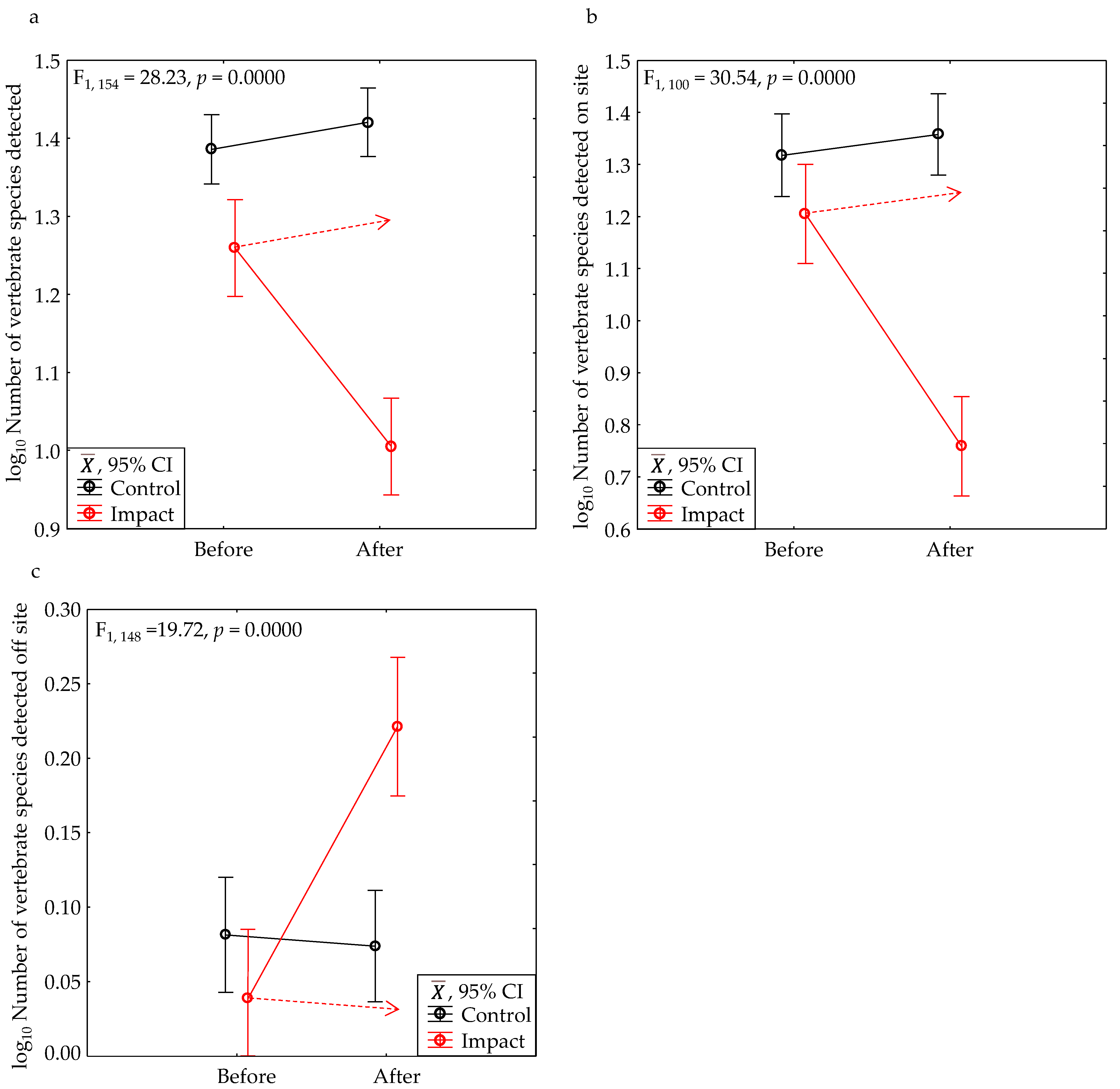
All vertebrates	Yes	0.6161	99.34	0.0000	16.31	0.0001	28.23	0.0000	1.00
Onsite vertebrates	Yes	0.7228	65.44	0.0000	21.31	0.0000	30.54	0.0000	1.00
Offsite vertebrates	Yes	0.0002	5.98	0.0163	16.71	0.0001	19.72	0.0000	0.99
All birds	Yes	0.7747	84.00	0.0000	12.52	0.0005	23.90	0.0000	1.00
Onsite birds	Yes	0.6205	49.67	0.0000	15.93	0.0001	26.42	0.0000	1.00
All mammals	Yes	0.0600	8.52	0.0043	0.60	0.4408	0.03	0.8560	0.05
Onsite mammals	Yes	0.1827	5.78	0.0192	1.20	0.2783	0.60	0.4402	0.12
All herps	Yes	1.0000	3.07	0.0888	0.01	0.9104	0.01	0.9104	0.05
Onsite herps
All non-birds	Yes	0.0622	14.50	0.0002	1.19	0.2770	0.56	0.4576	0.11
Onsite non-birds	Yes	0.0837	4.24	0.0436	0.71	0.4029	0.47	0.4947	0.10
All special-status species	Yes	0.6230	46.00	0.0000	12.18	0.0006	12.18	0.0006	0.93
Onsite special-status species	Yes	0.2806	12.05	0.0008	5.26	0.0242	4.71	0.0327	0.57
Model-predicted at 1 h	Yes	0.2336	37.04	0.0000	4.06	0.0459	10.32	0.0017	0.89
Unique species per survey	Yes	0.7910	24.05	0.0000	36.01	0.0000	71.50	0.0000	1.00
Animals counted
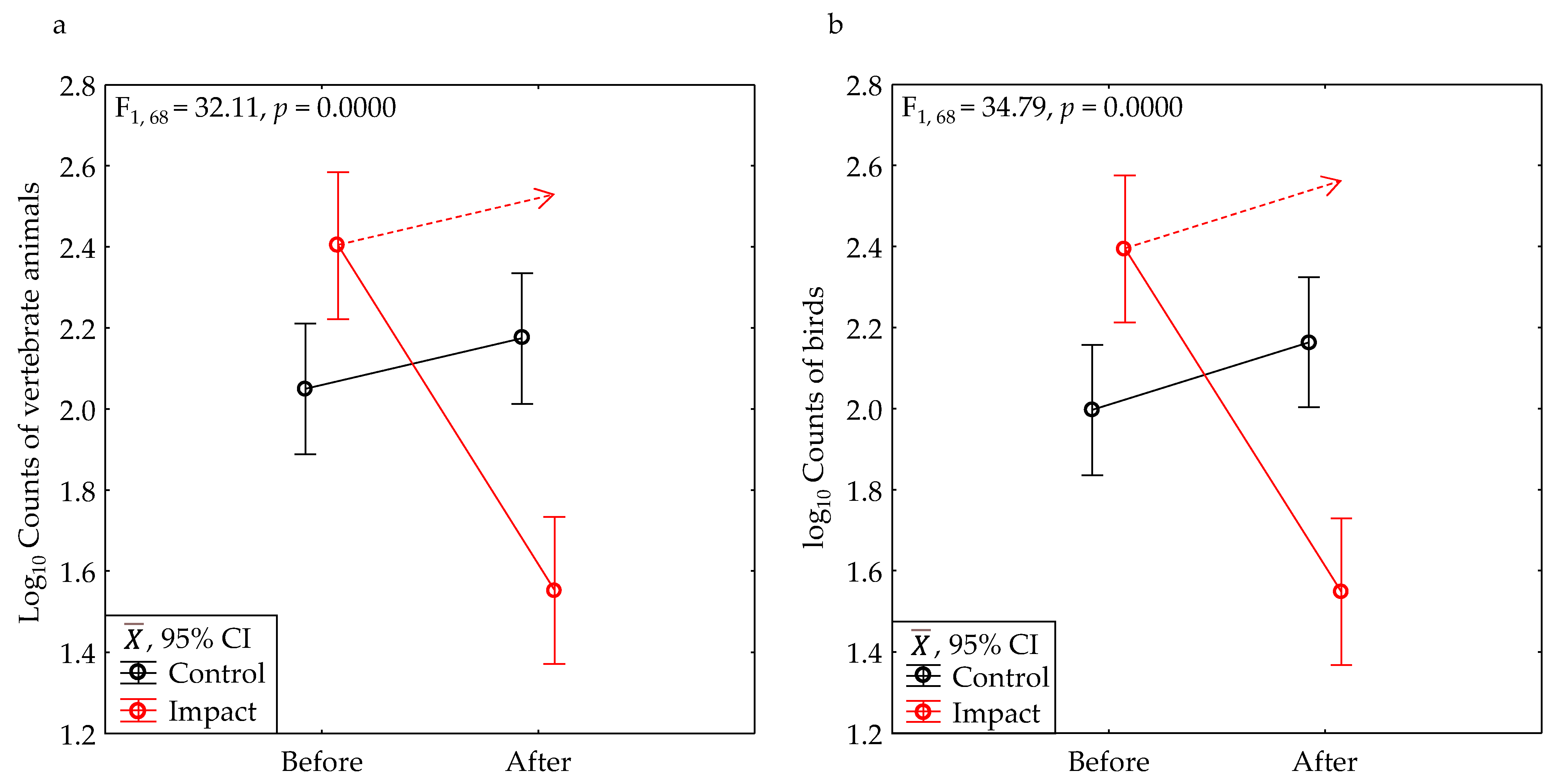
All vertebrates	Yes	0.2890	2.44	0.1235	17.80	0.0001	32.11	0.0000	1.00
Onsite vertebrates	Yes	0.0035	0.02	0.8842	7.40	0.0088	11.77	0.0012	0.92
All birds	Yes	0.2916	1.62	0.2076	15.63	0.0002	34.79	0.0000	1.00
Onsite birds	Yes	0.0040	0.00	0.9964	6.68	0.0126	11.86	0.0011	0.92
All special-status species	Yes	0.8945	1.96	0.1672	10.11	0.0023	4.76	0.0331	0.57
Onsite special-status species	Yes	0.8629	0.84	0.3647	9.87	0.0030	6.15	0.0171	0.68

Table 4. Mean number of species detected per survey in each identified species’ group among the surveys in the experimental treatment groups of control-before, control-after, impact-before, and impact-after. Measures of the percentage effect of development appear in the right column.

Group	Control (n = 52)		Impact (n = 26)		Effect (%)
Group	Before	After	Before	After	Effect (%)
Birds	23.1	25.73	17.73	10.19	−48
Mammals	2.52	2.42	1.38	0.19	−86
Reptiles	0.33	0.33	0.08	0.08	0
Amphibians	0.06	0.4	0.04	0	−100
Special-status species	5.11	4.88	3.69	1.81	−49
Non-native birds	1.98	2.37	2.69	1.81	−44
Synanthropic birds	7.19	7.67	7.42	5.73	−28
Raptors	2.77	2.61	2.58	1.15	−53
Grassland birds	1.9	1.81	1.5	0.36	−75

Disclaimer/Publisher’s Note: The statements, opinions and data contained in all publications are solely those of the individual author(s) and contributor(s) and not of MDPI and/or the editor(s). MDPI and/or the editor(s) disclaim responsibility for any injury to people or property resulting from any ideas, methods, instructions or products referred to in the content.

© 2023 by the authors. Licensee MDPI, Basel, Switzerland. This article is an open access article distributed under the terms and conditions of the Creative Commons Attribution (CC BY) license (https://creativecommons.org/licenses/by/4.0/).

Share and Cite

MDPI and ACS Style

Smallwood, K.S.; Smallwood, N.L. Measured Effects of Anthropogenic Development on Vertebrate Wildlife Diversity. Diversity 2023, 15, 1037. https://doi.org/10.3390/d15101037

AMA Style

Smallwood KS, Smallwood NL. Measured Effects of Anthropogenic Development on Vertebrate Wildlife Diversity. Diversity. 2023; 15(10):1037. https://doi.org/10.3390/d15101037

Chicago/Turabian Style

Smallwood, K. Shawn, and Noriko L. Smallwood. 2023. "Measured Effects of Anthropogenic Development on Vertebrate Wildlife Diversity" Diversity 15, no. 10: 1037. https://doi.org/10.3390/d15101037

Note that from the first issue of 2016, this journal uses article numbers instead of page numbers. See further details here.

Article Menu

Measured Effects of Anthropogenic Development on Vertebrate Wildlife Diversity

Abstract

1. Introduction

2. Materials and Methods

2.1. Study Area

2.2. Reconnaissance Surveys

2.3. BACI Tests

2.4. Effects of Other Factors

2.5. Species Characteristics

3. Results

3.1. BACI Experiment

3.2. Effects of Other Factors

3.3. Species Characteristics

4. Discussion

4.1. Effects of Development on Vertebrate Wildlife

4.2. Landscape Effects

4.3. Evidence of Ongoing Cumulative Effects of Urbanization

4.4. Potential Biases

5. Conclusions

Author Contributions

Funding

Data Availability Statement

Acknowledgments

Conflicts of Interest

Appendix A

References

Share and Cite

Article Metrics

Article Access Statistics

Further Information

Guidelines

MDPI Initiatives

Follow MDPI