Article

Distribution and Environmental Impact Factors of Phytoplankton in the Bay of Bengal during Autumn

1
College of Food Science and Engineering, Tianjin University of Science and Technology, Tianjin 300457, China
2
Research Centre for Indian Ocean Ecosystem, Tianjin University of Science and Technology, Tianjin 300457, China
3
College of Marine Science and Technology, China University of Geosciences (Wuhan), Wuhan 430074, China
4
State Key Laboratory of Biogeology and Environmental Geology, China University of Geosciences (Wuhan), Wuhan 430074, China
*
Author to whom correspondence should be addressed.
Diversity 2022, 14(5), 361; https://doi.org/10.3390/d14050361
Submission received: 18 March 2022 / Revised: 19 April 2022 / Accepted: 19 April 2022 / Published: 3 May 2022

Abstract

:
In order to better understand the effects of environmental factors and water mixing on the phytoplankton community structure in the Bay of Bengal, a field investigation was conducted from October to December 2016. A total of 276 species from 68 genera were identified, including Bacillariophyta (81 species), Miozoa (188 species), Cyanobacteria (four species), and Ochrophyta (three species). The abundance and distribution of dominant cyanobacteria gradually decreased along the latitude. This is evidenced in the vertical direction, which shows that cyanobacteria were affected by changes in environmental factors caused by the vertical mixing of seawater. The relationship between stratified N:P and phytoplankton also revealed that the changes in the vertical direction of the water deeply affected the phytoplankton community structure in the Bay of Bengal. The regions with strong vertical stratification were more favorable for the growth of cyanobacteria, while the regions with weak vertical stratification were more favorable for the growth of diatoms and dinoflagellates. According to the canonical correspondence analysis, nitrogen, silicates, phosphates, vertical stratification, and temperature were key control factors for phytoplankton communities. However, changes in these chemical parameters in the study area were also caused by the seawater cycle process.

1. Introduction

As primary producers in the ocean, phytoplankton contribute nearly 50% of global primary production [1] and play important roles in biogeochemical cycling and the global carbon cycle [2]. Phytoplankton are the major producers and food sources of marine ecosystems [3]. Moreover, in marine ecosystems, phytoplankton diversity has a stabilizing effect on ecosystem function and is the best predictor for resource use efficiency under considerable environmental gradients [4]. Therefore, understanding phytoplankton diversity can help in assessing the importance of phytoplankton in the functioning of marine ecosystems. Different functional groups of phytoplankton are involved in marine primary productivity [5], marine biological resource biomass [6], food web stability [7], and biological pump efficiency [8,9]. Therefore, the importance of marine ecosystem functions can be assessed using phytoplankton diversity. As major producers under different hydrological conditions [10], phytoplankton are also important to productivity in the oligotrophic Bay of Bengal (BOB) and play an important role in the final biogeochemical cycle. Most studies on BOB’s phytoplankton are based on remote sensing and modeling [11,12]. However, in situ observations of phytoplankton in the area are rare.
As an important carbon dioxide sink, the ocean plays a significant role in climate change and in buffering rising atmospheric carbon dioxide (CO2). The BOB is located on the east coast of the mainland and forms the main part of the northern Indian Ocean, with a latitude range between 5° N and 25° N. As the largest bay in the world, the BOB is a significant channel between the Pacific Ocean and the Indian Ocean. Due to the closed nature of the BOB and the influence of the tropical ocean basin, the cellular abundance of organisms in the water body of the BOB is much lower than that of the adjacent sea areas [13]. Studies have shown that rivers bring a lot of nutrients from land, making marine phytoplankton highly productive. However, there is a lack of vertical force mixing and high sediment load in this area, and the relatively low level of primary productivity in summer is related to the reduction in solar insolation due to excessive cloud thickness [14]. Since the BOB receives runoff from continental river systems and fresh water from oceanic precipitation [15], which substantially lowers the salinity, the distribution of phytoplankton in this area is greatly affected by river dilution. The BOB is influenced by the semi-annual seasonality of the Asian monsoon system, which is characterized by two distinct monsoon periods, the winter monsoon (WiM) [16] and the summer monsoon (SuM) [17]. During the dry, relatively calm WiM (November to February), northeasterly winds dominate, while the SuM (June to September) is characterized by higher precipitation and stronger southwesterly winds. However, how this changing environmental driver affects the phytoplankton community structure in the BOB is unclear, as resources are currently scarce. Therefore, in order to maintain the stability of BOB marine ecosystems and resources, it is necessary to study ecological dynamic mechanisms and key environmental factors. Here, we present a detailed study on the phytoplankton community in the autumn to assess (i) the phytoplankton community’s structure in the BoB and (ii) the influence of hydrography and environmental factors on the phytoplankton distribution.

2. Methods

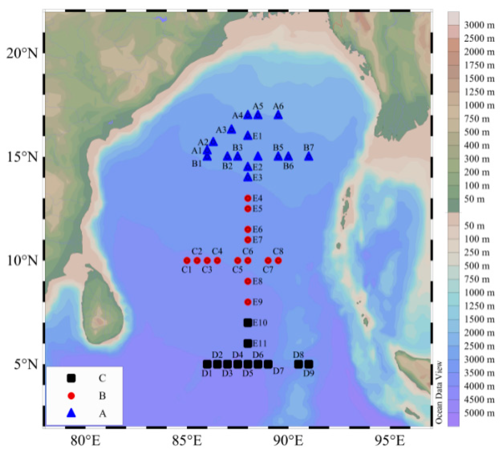
2.1. Sampling and Analysis

Water samples were collected on the R/V ‘Dong Fang Hong 2 in October–December 2016 from 41 sampling stations covering the Bay of Bengal in the Indian Ocean (82.00° E–95.00° E, 4.00° N–18.00° N) (Figure 1). At each station, the sampling depths were 5, 30, 75, 100, 150, and 300 m. Phytoplankton samples from different water layers were stored in 1000 mL polyethylene bottles and fixed in formaldehyde solution (3%). At each sampling station, the Seabird CTD was used to record the temperature, salinity, and fluorescence intensity of the seawater.
For laboratory analysis, the Utermöhl method was used, and the water samples were concentrated in a 100 mL sedimentation column for 24 to 48 h. The identification and counting of the phytoplankton cells were conducted by inverted microscope at 400× (or 200×). The methods of Jin [18], Yamaji [19], and Sun [20] were used to determine the species of phytoplankton.
In situ seawater was filtered through a 0.45 µm cellulose acetate membrane and then refrigerated at 4 °C for nutrient analysis. A Technicon AA3 Auto-Analyzer (Bran + Luebbe) was used to detect ammonium, nitrate, phosphate, and silicic. The method of phosphomolybdenum blue was used to determine soluble inorganic phosphorus (PO4-P), the method of molybdenum blue was used to determine soluble silicate (SiO3-Si), the method of cadmium column was used to determine nitrate (NO3-N), the method of naphthylethylenediamine was used to determine nitrite (NO2-N), and the method of sodium salicylate was used to determine ammonia (NH4-N) [21,22,23].

2.2. Data Analysis and Statistical Methods

The dominance index (Y) was calculated to describe the species dominance in the phytoplankton community. The calculation equation for [24]:
Y = n i N   · fi
where ni is the number of cells of species i, N is the total number of individuals in the collected samples, and fi is the frequency of occurrence of species i in each sample.
The abundance of phytoplankton cells in the water column was calculated through the trapezoidal integral method [25]:
P = { i = 1 n 1 P i + 1 + P i 2 ( D i + 1 D i ) } / D
where P is the average phytoplankton abundance in water column, Pi is the abundance value of phytoplankton in layer i, D is the maximum sampling depth, Di is the depth of layer i, and N is the sampling level.
To quantify the stratification strength of the upper ocean, the vertical stratification index (VSI) was used to focus on changes in ocean temperature and salinity, i.e., the change in the density stratification [26]:
VSI = [ δ σ ( m + 1 ) δ σ ( m ) ]  
where δσ is the potential density anomaly, and m is the depth from 5 to 300 m.
Canonical correspondence analysis (CCA) and redundancy analysis (RDA) were used to analyze the relationship between phytoplankton and environmental factors. Discriminant component analysis (DCA) was used to select CCA and RDA; if axis lengths were >4, CCA was selected, if axis lengths were <3, RDA was selected, if 4 > axis lengths > 3, both CCA and RDA could be used. Cluster analysis (Primer 6.0) was used for the similarity analysis of the phytoplankton community structure. The distribution of the phytoplankton and a correlation analysis with the environment were performed using Ocean Data View 4.10, Original 8.5, Arc GIS 10.2, and R 4.1.0.

3. Results

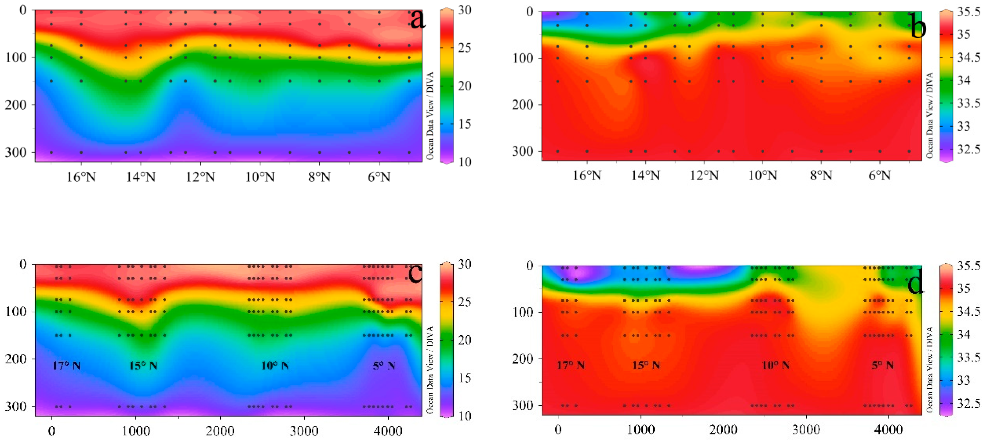
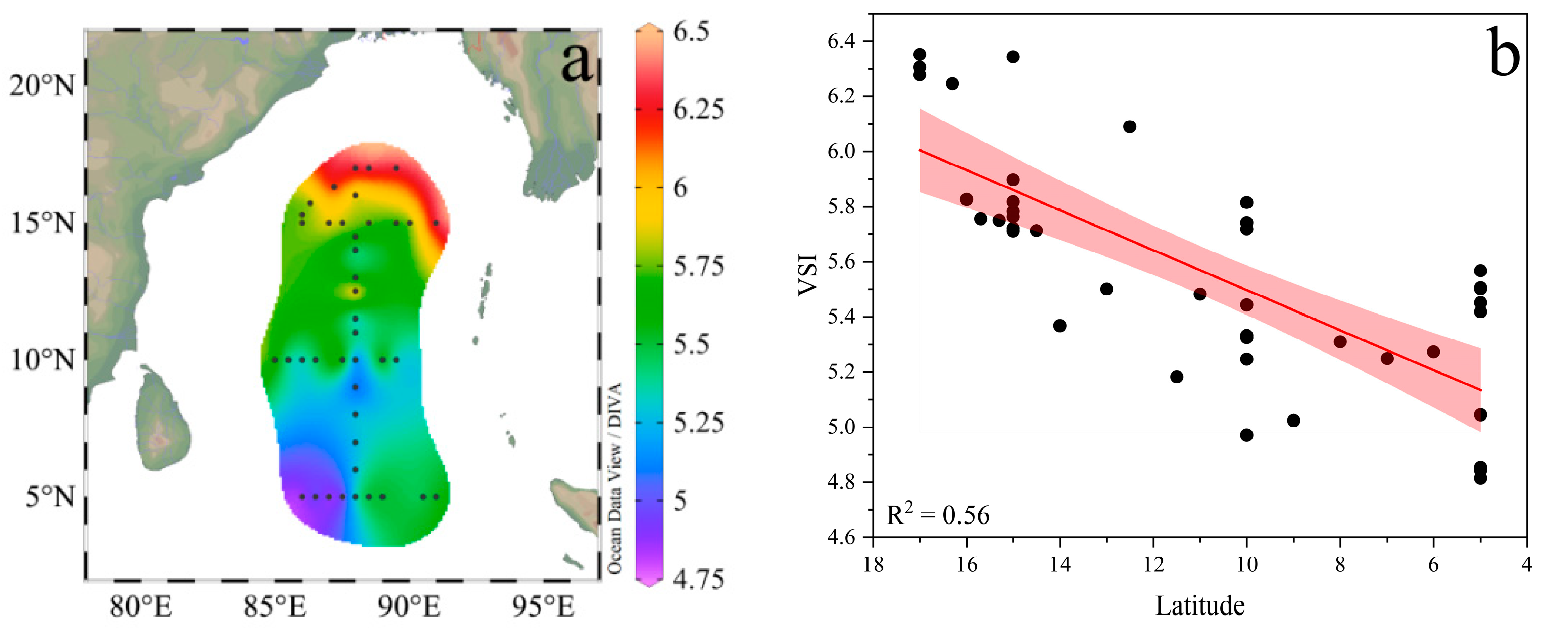
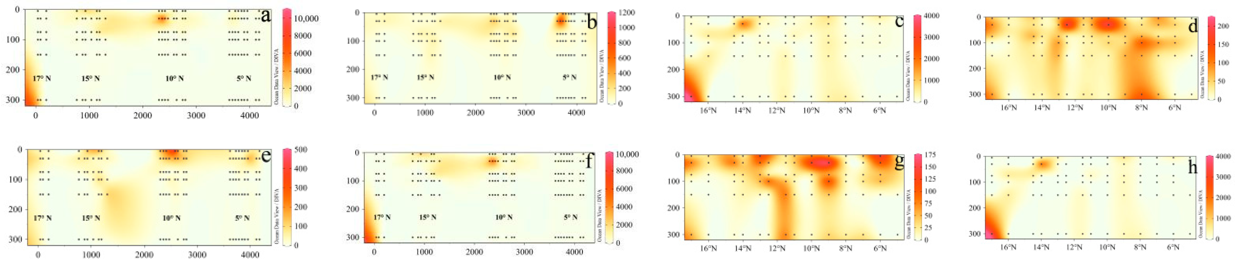
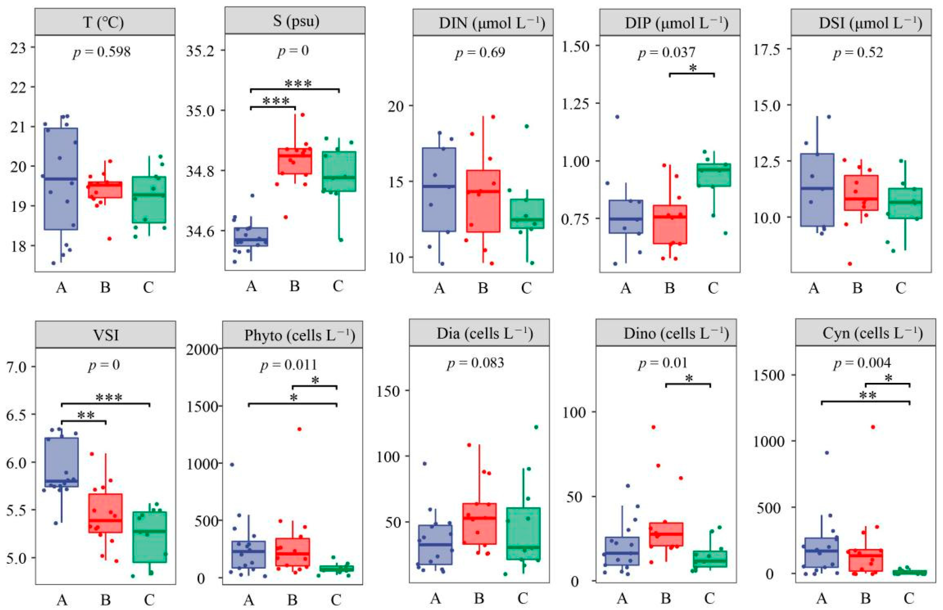
3.1. Environmental Parameters

The temperature of the surveyed area ranged from 11.31 ℃ to 29.39 ℃, with an average of 22.42 ℃; the salinity of the surveyed area ranged from 32.31 psu to 35.31 psu, with an average of 34.46 psu. There was an obvious high temperature and low salinity region at 15° N. In the vertical distribution, the temperature decreased with increasing depth, and the salinity increased from the surface layer to the bottom (Figure 2a–d). The difference in temperature and salinity was mainly at 15° N, and the seawater stratification in the survey area was obvious. The temperature above the 100-m depth layer in the survey area was significantly higher than that below the 100 m depth layer, and the salinity was significantly lower in the area above the 75-m depth layer north of 12° N due to the influence of diluted water.
The vertical stratification index (VSI) of the surveyed area is shown in Figure 3. The highest value of VSI appears at 16.5° N and decreases with decreasing latitude. The minimum value appeared at 5° N, with an average value of 6.5. The horizontal distribution of VSI showed higher VSI in nearshore areas and lower VSI in areas close to the open ocean. This further indicated that the degree of mixing of seawater in the north of the Bay of Bengal was gradually increasing.

3.2. Species Composition and Dominant Species

A total of 276 species (68 genera and 4 phyla) of phytoplankton were identified across the BOB. A total of 188 Miozoa species were accurately discriminated, representing 68.11% of the total phytoplankton taxa. Thus, Miozoa were a highly diverse group of phytoplankton in the BOB. Bacillariophyta were the second most diverse group (81 species), accounting for 29.34% of the total species. Species in other groups (Cyanophyta, Cyanobacteria, and Ochrophyta) were recorded more sparsely and only accounted for about 2.54% of the total species. The most species-rich genera in the BOB were Chaetoceros (14 species) and Rhizosolenia (9 species) for diatoms and Ceratium (55 species) and Protoperdinium (24 species) for dinoflagellates. In this investigation, the cyanobacteria belonged to two genera and four species. Additionally, Richelia intracellularis appeared in two lifestyles, i.e., free living and extracellular endosymbiosis with Rhizosolenia styliformis.
The dominant taxa in the BOB belonged to Bacillariophyta (six species), Miozoa (two species), Cyanobacteria (one species), and Ochrophyta (one species) (Table 1). In particular, the chain-forming diatoms, Trichodesmium spp., became the most common dominant species and were mainly distributed in the water layer above 75 m. The cell abundance of Trichodesmium spp. was between not detected (ND) and 9.00 × 10³ cells/L. The maximum cell abundance of Trichodesmium spp. was observed 30 m deep at Station C2 (Figure 4). Most of these species were tropical species and warm-water species, which is consistent with the tropical climate characteristics of this sea area.

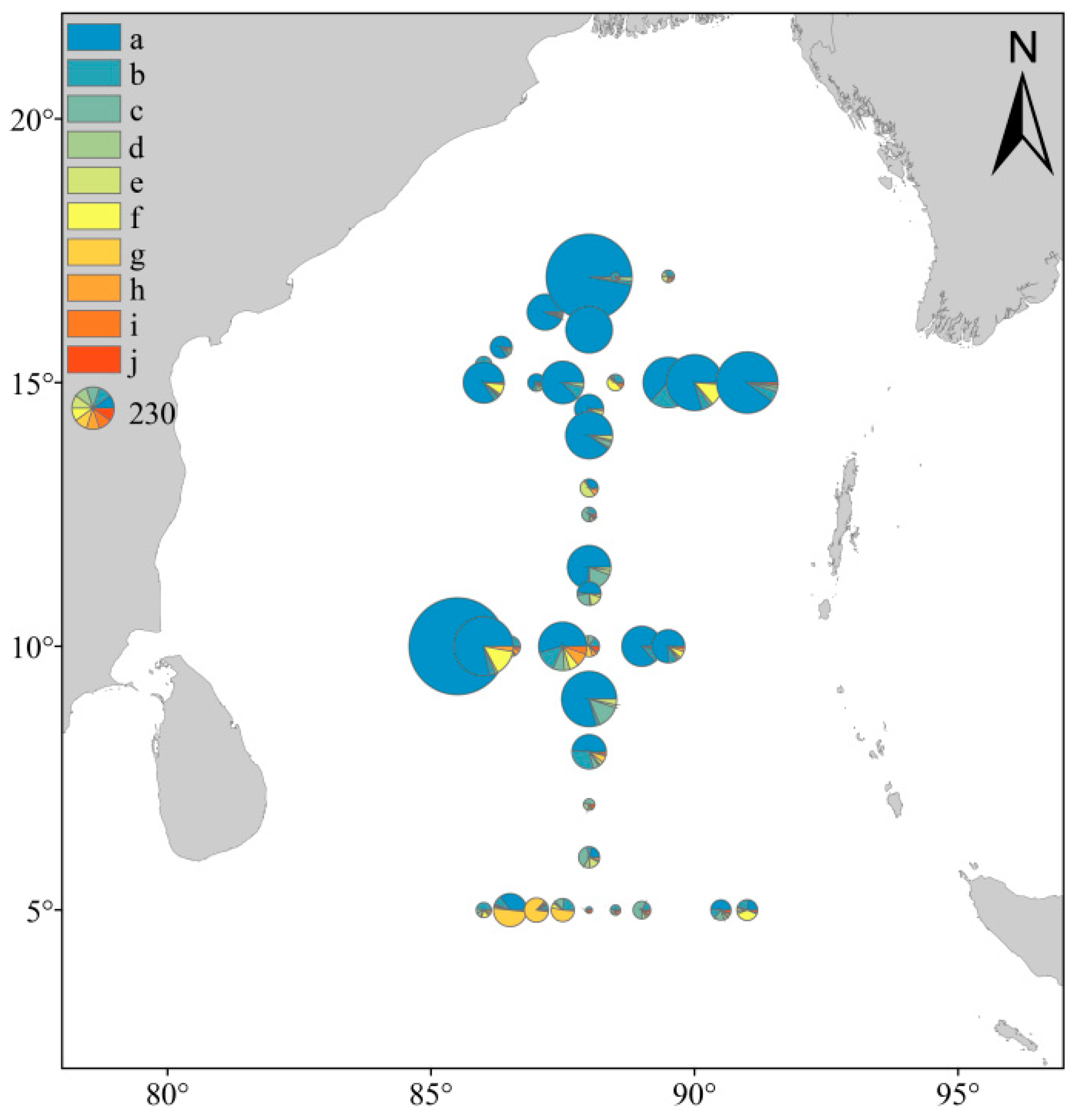
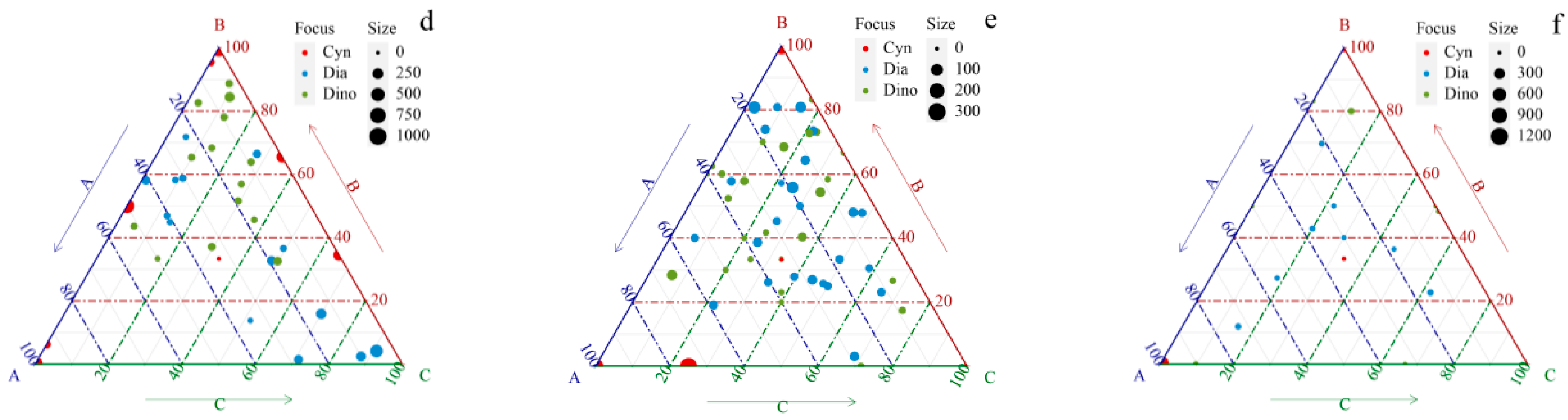
3.3. Distribution of Phytoplankton Community Structure

The transect distribution of phytoplankton is shown in Figure 5. The distribution of phytoplankton groups was patchy. The transect distribution of phytoplankton varied greatly. The distribution of phytoplankton is mainly determined by cyanobacteria, and the dominant species was Trichodesmium spp. In the bottom layer of 17° N, there was a large number of Trichodesmium spp., which may have been caused by the deposition of Trichodesmium spp. in the upper layer after the mass reproduction. Diatoms and dinoflagellates were evenly distributed in the water, with increasing cell abundance from north to south. The vertical variation of total phytoplankton was similar to that of cyanobacteria. At the same latitude, there was little change in the phytoplankton groups. Diatoms and dinoflagellates were mainly distributed in the upper layer of the water body, while Trichodesmium spp. decreased gradually with the decrease in latitude.
The change in the average abundance and percentage of phytoplankton between different latitudes is shown in Figure 6a. The abundance of phytoplankton in C1 was the highest, while the abundance of phytoplankton in D5 was the lowest. Between 8° N and 17° N, cyanobacteria dominated the distribution of phytoplankton, and the cell abundance of diatoms gradually increased. Cluster analysis was used to analyze the community structure of phytoplankton. Combining geographic location and environmental factors, we divided the survey area into three sub-regions (Figure 1); sub-region A was in the northern part of the Bay of Bengal, sub-region B was in the central part of the Bay of Bengal, and sub-region C was in the southern part of the Bay of Bengal.
Based on the results of the cluster analysis, we calculated the differences in environmental factors and phytoplankton between regions. The environmental factors and phytoplankton communities of the three regions and their differences are shown in Figure 7. For environmental factors, there were significant differences between regions. The salinity in sub-region A was significantly lower than in sub-regions B and C, and the concentration of phosphate in sub-region C was higher than in sub-regions A and B. The VSI in sub-region C was higher than in sub-regions A and B. For phytoplankton communities, the differences were mainly caused by dinoflagellates, Cyanobacteria, and diatoms in the surveyed area. The most obvious difference was that the cyanobacteria in sub-regions A and B were significantly higher. The phytoplankton abundance in sub-regions A and B was significantly higher in the whole community structure.

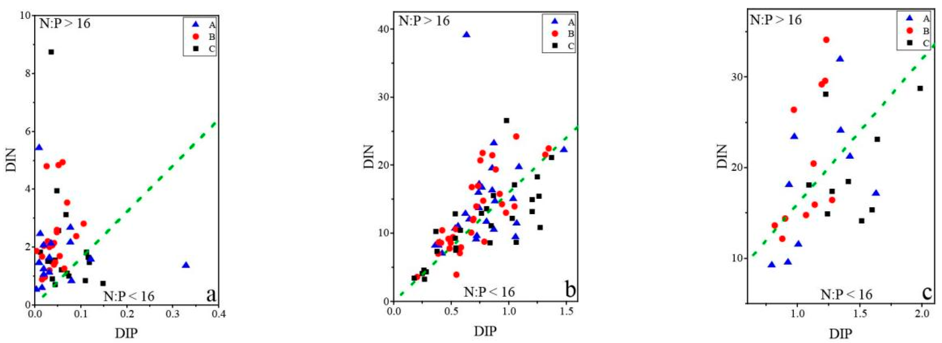
3.4. Relationships between Phytoplankton and Environmental Factors

We compared the N:P ratios of the surface, middle, and bottom layers. The N:P ratio in the surface layer (N:P > 16:1) indicated phosphorus limitation. In the middle and bottom layers, the N:P = 16:1, indicating that the nutrient ratio was stable. As the depth increased, the concentration of nutrients gradually increased, but the abundance of phytoplankton gradually decreased, indicating that the influence of light was greater than that of nutrients in the bottom layer. Phosphorus limitation was more obvious in the surface layer of sub-regions A and B than in sub-region C (Figure 8a). In the middle and bottom layers, although the N:P of the three regions still showed certain fluctuations, nutrients were no longer a limiting factor for phytoplankton growth with the increase in depth. According to the ternary diagram, cyanobacteria were mainly distributed in sub-regions A and B on the surface, while diatoms were mainly distributed in sub-region C. Diatoms and dinoflagellates were the dominant species in the middle layer and were evenly distributed in this area. The abundance of phytoplankton in the bottom layer was low and distributed evenly among the three sub-regions, while cyanobacteria were distributed mostly in sub-region A (Figure 8b,c).
Discriminant component analysis (DCA) was used to select a suitable correlation analysis. According to the results, canonical correlation analysis (CCA) was used to analyze the relationship between the dominant species and the environmental factors. The results of the correlation analysis showed that Trichodesmium spp. was negatively correlated with nutrients and positively correlated with temperature. The Tripos furca in dinoflagellates was consistent with Trichodesmium spp., and the diatoms in dominant species were positively correlated with salinity and nutrients. Correlations between species and environmental factors were analyzed using redundancy analysis (RDA) (Figure 9b). The results showed obvious differences between different phytoplankton and environmental factors. The correlation between various groups and the environment was highly consistent with the dominant species. Cyanobacteria and dinoflagellates were negatively correlated with nutrients and positively correlated with VSI, indicating that cyanobacteria (especially Trichodesmium spp.) were more suitable for growing in waters with high VSI. Diatoms were positively correlated with temperature and salinity and negatively correlated with VSI and nutrients, suggesting that waters with low VSI were more suitable for diatoms. There were three phytoplankton community sub-regions in the BOB. Sub-region A was distributed in the northern part of BOB, with obvious vertical stratification. The abundance of sub-region A was high and was dominated by Trichodesmium spp. Sub-region B was located near 10° N, and the phytoplankton community was dominated by warm-water species, similar to sub-region A. The difference was that the abundance of diatoms and dinoflagellates in sub-region B was higher than that in sub-region A. Sub-region C was located at 5° N, the VSI of sub-region C was low, and the phytoplankton community was dominated by diatoms. In sub-region C, the phytoplankton were positively correlated with nutrients.

4. Discussion

4.1. Hydrological Conditions and Corresponding Phytoplankton Community Structure

The survey area covered a wide range from the northern part of the Bay of Bengal to the equator. The salinity varies greatly along the latitude, indicating that the environmental factors in the BOB change greatly, and the nutrient difference was obvious. The main factors affecting the distribution of the phytoplankton community included physical factors, chemical factors, and biological factors [27]. The dependence of diatoms and dinoflagellates on environmental factors was reflected by their relative position in the RDA biplot. The results of the correlation analysis showed that sub-regions A and B were greatly affected by temperature and VSI. There were more cyanobacteria and dinoflagellates in sub-regions A and B, which may be due to the strong adaptability of cyanobacteria and dinoflagellates to temperature. The salinity in sub-region C was high due to the intrusion of high-salinity ocean water. The temperature was higher, the abundance of diatoms was lower, and the abundance of dinoflagellates and cyanobacteria was higher in sub-regions A and B. The adaptation of diatoms, dinoflagellates, and cyanobacteria to oligotrophic sea areas determines the community structure of phytoplankton [28,29]. In our survey area, the phytoplankton community structure and abundance showed a trend of gradual change along the latitudinal section. Although some mesoscale eddies and secondary mesoscale eddies may lead to the instability of local waters, the spatial distribution of diatoms remained stable along the nutrient gradient within a certain period. There were differences in the phytoplankton community structure in the survey area. The abundance of cyanobacteria in sub-region C was extremely low. The average abundance in sub-region B was higher than in sub-regions A and C. The abundance of diatoms in sub-region B was high. Sub-region B was affected by the mixing of dilute water and seawater, which can bring high amounts of nutrients to the surface, promoting diatom reproduction [30]. The growth and reproduction of dinoflagellates will be more inhibited in an environment with severe circulation and eddy currents. Vigorous water exchange inhibits the cell division and absorption of nutrients by dinoflagellates, in addition to destroying their cell morphologies [31,32]. The results of the correlation analysis of phytoplankton communities also showed that diatoms were positively correlated with nutrients and that cyanobacteria and dinoflagellates were positively correlated with temperature. The correlation analysis between the top 10 dominant species and the environment also confirmed that cyanobacteria and dinoflagellates were significantly positively correlated with temperature, while diatoms were mainly positively correlated with nutrients. Historical investigations have shown that Trichodesmium spp. is suitable for living at temperatures of 20–30 ℃, and the surface temperature in our survey area was relatively high [33,34]. Our results also showed that temperature has a great influence on the spatial distribution of Trichodesmium spp.

4.2. Vertical Stratification and Phytoplankton Community Structure

The factors that control the phytoplankton community structure in natural sea areas have been studied for many years, but there are few studies on the limitations of phytoplankton community structures due to nutrient concentrations and ratios [35]. Diatoms and dinoflagellates differ widely in their cell morphologies and nutritional patterns. Numerous studies have shown that dinoflagellates use mixed nutrients, but the concentration of phosphate is a main factor limiting the production and reproduction of dinoflagellates. Diatom’s absorption of nutrients is relatively simple, and its growth and reproduction are restricted by more factors [36,37]. In conclusion, fluctuations in physical and chemical environmental parameters profoundly affect the community structure of phytoplankton.
In the marine ecological environment, nutrients are an important factor in determining the phytoplankton community. The stratification was obvious in the investigation area. The vertical stratification of the survey area determined the distribution of environmental factors such as nutrients and then influenced the community structure of the phytoplankton. In our study, N:P > 16 in the surface layer of sub-regions A and B indicated that these two sub-regions were phosphorus-limited and that the abundance of Trichodesmium spp. in the surface layer of these two regions was very high. N:P < 16 in sub-region C, and thus the abundance of diatoms increased. With the increase in nutrient concentration, the N:P in the middle layer was relatively stable (N:P = 16). In the middle layer, there were mainly diatoms and the distribution was relatively uniform. Nutrients were higher in the bottom layer, and phytoplankton were limited by light rather than nutrients, so the abundance of phytoplankton was lower.
The changes in physical and chemical processes are an integrated response to vertical stratification, and the distribution of phytoplankton is in turn a response to physical and chemical processes. The results of this study indicate that the process of VSI reduction with latitude is accompanied by a transition of the phytoplankton community structure from cyanobacteria to diatoms. The abundance of Trichodesmium determined the difference in the abundance of phytoplankton in the surveyed area at different sub-regions and depths. Our results show that the highly stratified region was more suitable for the growth of dinoflagellates and Trichodesmium, while the region with low vertical stratification seemed to be more conducive to diatoms (Figure 6 and Figure 9). This is mainly due to the fact that dinoflagellates and Trichodesmium are better suited to living in stable waters, while diatoms are better suited to living in mixed waters with high nutrient levels [38]. Weak vertical stratification resulted in a more uniform vertical distribution of temperature, salinity, density, and nutrients in sub-region C (Figure 9b) [39]. VSI gradually decreased with latitude, and the correlation analysis results show that diatoms were positively correlated with nutrients, which indicates that the change in VSI was an important factor affecting the change in nutrient levels (N:P). The high VSI on the surface of the Bay of Bengal inhibits the exchange of seawater. This leads to a lack of nutrients and ultimately affects the distribution of phytoplankton.

5. Conclusions

This study investigated the phytoplankton community structure in the Bay of Bengal in autumn 2016, revealing spatial variations in the community composition and abundance of phytoplankton, as well as their relationship with physical ocean processes and environmental factors. The results of this comprehensive analysis show that the VSI is driven by temperature and salinity and caused differences in nutrients in different regions at different depths, which in turn affected the phytoplankton community structure. Although this study carried out an analysis of the phytoplankton in the Bay of Bengal, the study of the changes in phytoplankton in a small area is a process that requires long-term observation, so further exploration is still required.

Author Contributions

Conceptualization, J.S.; data curation, X.W.; formal analysis, X.W. and H.Y.; funding acquisition, J.S.; investigation, X.W.; resources, J.S.; supervision, J.S.; writing—original draft, X.W.; writing—review and editing, J.S. All authors have read and agreed to the published version of the manuscript.

Funding

This research was financially supported by National Nature Science Foundation of China grants (41876134 and 41676112), the Changjiang Scholar Program of Chinese Ministry of Education (T2014253) to Jun Sun, and State Key Laboratory of Biogeology and Environmental Geology, China University of Geosciences (No. GKZ21Y645).

Institutional Review Board Statement

Not applicable.

Informed Consent Statement

Not applicable.

Data Availability Statement

All data are available from the authors upon request.

Acknowledgments

We thank all the members of Dongfanghong 2 for supporting and securing our scientific investigation on this cruise. Thanks to the CTD data provided by Jiwei Tian’s team at Ocean University of China. Thanks to Ming Wang and Hongtao Chen for their assistance during the sampling and sample determination.

Conflicts of Interest

The authors declare no conflict of interest.

References

  1. Field, C.B.; Behrenfeld, M.J.; Randerson, J.T.; Falkowski, P. Primary production of the biosphere: Integrating terrestrial and oceanic components. Science 2016, 281, 237–240. [Google Scholar] [CrossRef] [PubMed] [Green Version]
  2. Falkowski, P.G.; Barber, R.T.; Smetacek, V. Biogeochemical controls and feedbacks on ocean primary production. Science 1998, 281, 200–206. [Google Scholar] [CrossRef] [PubMed] [Green Version]
  3. Schloss, I.R.; Abele, D.; Moreau, S.; Demers, S.; Bers, A.V.; González, O.; Ferreyra, G.A. Response of phytoplankton dynamics to 19-year (1991–2009) climate trends in Potter Cove (Antarctica). J. Mar. Syst. 2012, 92, 53–66. [Google Scholar] [CrossRef]
  4. Ptacnik, R.; Solimini, A.G.; Andersen, T.; Tamminen, T.; Brettum, P.; Lepistö, L.; Rekolainen, S. Diversity predicts stability and resource use efficiency in natural phytoplankton communities. Proc. Natl. Acad. Sci. USA 2008, 105, 5134–5138. [Google Scholar] [CrossRef] [Green Version]
  5. Deppeler, S.L.; Davidson, A.T. Southern Ocean phytoplankton in a changing climate. Front. Mar. Sci. 2017, 4, 40. [Google Scholar] [CrossRef] [Green Version]
  6. Loeb, V.; Hofmann, E.E.; Klinck, J.M.; Holm-Hansen, O. Hydrographic control of the marine ecosystem in the South Shetland-Elephant Island and Bransfield Strait region. Deep Sea Res. Part II Top. Stud. Oceanogr. 2010, 57, 519–542. [Google Scholar] [CrossRef]
  7. Forcada, J.; Trathan, P.N.; Boveng, P.L.; Boyd, I.L.; Burns, J.M.; Costa, D.P.; Southwell, C.J. Responses of Antarctic pack-ice seals to environmental change and increasing krill fishing. Biol. Conserv. 2012, 149, 40–50. [Google Scholar] [CrossRef] [Green Version]
  8. Kerr, R.; Goyet, C.; da Cunha, L.C.; Orselli, I.B.; Lencina-Avila, J.M.; Mendes, C.R.B.; Tavano, V.M. Carbonate system properties in the Gerlache Strait, Northern Antarctic Peninsula (February 2015): II. Anthropogenic CO2 and seawater acidification. Deep Sea Res. Part II Top. Stud. Oceanogr. 2018, 149, 182–192. [Google Scholar] [CrossRef]
  9. Tréguer, P.; Bowler, C.; Moriceau, B.; Dutkiewicz, S.; Gehlen, M.; Aumont, O.; Pondaven, P. Influence of diatom diversity on the ocean biological carbon pump. Nat. Geosci. 2018, 11, 27–37. [Google Scholar] [CrossRef]
  10. Platt, T.; Rao, D.V.; Irwin, B. Photosynthesis of picoplankton in the oligotrophic ocean. Nature 1983, 301, 702–704. [Google Scholar] [CrossRef]
  11. Vinayachandran, P.N.; Mathew, S. Phytoplankton bloom in the Bay of Bengal during the northeast monsoon and its intensification by cyclones. Geophys. Res. Lett. 2003, 30, 1572. [Google Scholar] [CrossRef] [Green Version]
  12. Vinayachandran, P.N.; McCreary, J.P., Jr.; Hood, R.R.; Kohler, K.E. A numerical investigation of the phytoplankton bloom in the Bay of Bengal during Northeast Monsoon. J. Geophys. Res. Ocean. 2005, 110, C12001. [Google Scholar] [CrossRef]
  13. Prasanna Kumar, S.; Nuncio, M.; Narvekar, J.; Kumar, A.; Sardesai, D.S.; De Souza, S.N.; Madhupratap, M. Are eddies nature’s trigger to enhance biological productivity in the Bay of Bengal? Geophys. Res. Lett. 2004, 31, L07309. [Google Scholar] [CrossRef] [Green Version]
  14. Li, G.; Ke, Z.; Lin, Q.; Ni, G.; Shen, P.; Liu, H.; Tan, Y. Longitudinal patterns of spring-intermonsoon phytoplankton biomass, species compositions and size structure in the Bay of Bengal. Acta Oceanol. Sin. 2012, 31, 121–128. [Google Scholar] [CrossRef]
  15. Liu, H.; Ke, Z.; Song, X.; Tan, Y.; Huang, L.; Lin, Q. Primary production in the Bay of Bengal during spring intermonsoon period. Shengtai Xuebao/Acta Ecol. Sin. 2011, 31, 7007–7012. [Google Scholar]
  16. Shetye, S.R.; Shenoi, S.S.C.; Gouveia, A.D.; Michael, G.S.; Sundar, D.; Nampoothiri, G. Wind-driven coastal upwelling along the western boundary of the Bay of Bengal during the southwest monsoon. Cont. Shelf Res. 1991, 11, 1397–1408. [Google Scholar] [CrossRef]
  17. Sengupta, D.; Bharath Raj, G.N.; Shenoi, S.S.C. Surface freshwater from Bay of Bengal runoff and Indonesian throughflow in the tropical Indian Ocean. Geophys. Res. Lett. 2006, 33, L22609. [Google Scholar] [CrossRef] [Green Version]
  18. Yamaji, I. Illustrations of the Marine Plankton of Japan; Hoikusha: Tokyo, Japan, 1996. [Google Scholar]
  19. Jin, D. Chinese Marine Planktonic Diatoms; Shanghai Scientific and Technical Publishers: Shanghai, China, 1965. [Google Scholar]
  20. Sun, J.; Liu, D.Y. The preliminary notion on nomenclature of common phytoplankton in China Seas waters. Oceanol. Limnol. Sin. 2002, 33, 271–286. [Google Scholar]
  21. Pai, S.C.; Tsau, Y.J.; Yang, T.I. pH and buffering capacity problems involved in the determination of ammonia in saline water using the indophenol blue spectrophotometric method. Anal. Chim. Acta 2001, 434, 209–216. [Google Scholar] [CrossRef]
  22. Dai, M.; Wang, L.; Guo, X.; Zhai, W.; Li, Q.; He, B.; Kao, S.J. Nitrification and inorganic nitrogen distribution in a large perturbed river/estuarine system: The Pearl River Estuary, China. Biogeosciences 2008, 5, 1227–1244. [Google Scholar] [CrossRef] [Green Version]
  23. Guo, S.; Feng, Y.; Wang, L.; Dai, M.; Liu, Z.; Bai, Y.; Sun, J. Seasonal variation in the phytoplankton community of a continental-shelf sea: The East China Sea. Mar. Ecol. Prog. Ser. 2014, 516, 103–126. [Google Scholar] [CrossRef] [Green Version]
  24. Sun, R. The Principle of Animal Ecology; Beijing Normal University Press: Beijing, China, 1987. [Google Scholar]
  25. Tan, J.Y.; Huang, L.M.; Tan, Y.H.; Lian, X.P.; Hu, Z.F. The influences of water-mass on phytoplankton community structure in the Luzon strait. Acta Oceanol. Sin. 2013, 35, 178–189. [Google Scholar]
  26. Mena, C.; Reglero, P.; Hidalgo, M.; Sintes, E.; Santiago, R.; Martín, M.; Moyà, G.; Balbín, R. Phytoplankton community structure is driven by stratification in the oligotrophic mediterranean sea. Front. Microbiol. 2019, 10, 1698. [Google Scholar] [CrossRef] [Green Version]
  27. Sun, J.; Song, S.Q.; Le, F.F.; Wang, D.; Dai, M.H.; Ning, X.R. Phytoplankton in northern South China Sea in the winter of 2004. Acta Oceanol. Sin. 2007, 29, 132–145. [Google Scholar]
  28. Busseni, G.; Rocha Jimenez Vieira, F.; Amato, A.; Pelletier, E.; Pierella Karlusich, J.J.; Ferrante, M.I.; Iudicone, D. Meta-omics reveals genetic flexibility of diatom nitrogen transporters in response to environmental changes. Mol. Biol. Evol. 2019, 36, 2522–2535. [Google Scholar] [CrossRef] [Green Version]
  29. Caputi, L.; Carradec, Q.; Eveillard, D.; Kirilovsky, A.; Pelletier, E.; Pierella Karlusich, J.J.; Tara Oceans Coordinators. Community-level responses to iron availability in open ocean plankton ecosystems. Glob. Biogeochem. Cycles 2019, 33, 391–419. [Google Scholar] [CrossRef]
  30. Estrada, M.; Berdalet, E. Phytoplankton in a turbulent world. Sci. Mar. 1997, 61, 125–140. [Google Scholar] [CrossRef]
  31. Thomas, W.H.; Gibson, C.H. Quantified small-scale turbulence inhibits a red tide dinoflagellate, Gonyaulax polyedra Stein. Deep Sea Res. Part A Oceanogr. Res. Pap. 1990, 37, 1583–1593. [Google Scholar] [CrossRef]
  32. Smayda, T.J. Harmful algal blooms: Their ecophysiology and general relevance to phytoplankton blooms in the sea. Limnol. Oceanogr. 1997, 42, 1137–1153. [Google Scholar] [CrossRef]
  33. Stal, L.J.; Severin, I.; Bolhuis, H. The ecology of nitrogen fixation in cyanobacterial mats. In Recent Advances in Phototrophic Prokaryotes; Springer: Cham, Switzerland, 2010; pp. 31–45. [Google Scholar] [CrossRef]
  34. Zehr, J.P.; Ward, B.B. Nitrogen cycling in the ocean: New perspectives on processes and paradigms. Appl. Environ. Microbiol. 2002, 68, 1015–1024. [Google Scholar] [CrossRef] [Green Version]
  35. Gao, K.; Beardall, J.; Häder, D.P.; Hall-Spencer, J.M.; Gao, G.; Hutchins, D.A. Effects of ocean acidification on marine photosynthetic organisms under the concurrent influences of warming, UV radiation, and deoxygenation. Front. Mar. Sci. 2019, 6, 322. [Google Scholar] [CrossRef]
  36. Huang, B.; Ou, L.; Hong, H.; Luo, H.; Wang, D. Bioavailability of dissolved organic phosphorus compounds to typical harmful dinoflagellate Prorocentrum donghaiense Lu. Mar. Pollut. Bull. 2005, 51, 838–844. [Google Scholar] [CrossRef] [PubMed]
  37. Stoecker, D.K. Mixotrophy among Dinoflagellates 1. J. Eukaryot. Microbiol. 1999, 46, 397–401. [Google Scholar] [CrossRef]
  38. Tilman, D. Green, blue-green and diatom algae: Taxonomic differences in competitive ability for phosphorus, silicon and nitrogen. Arch. Hydrobiol. 1986, 106, 473–485. [Google Scholar] [CrossRef]
  39. Pérez, V.; Fernández, E.; Marañón, E.; Morán, X.A.G.; Zubkov, M.V. Vertical distribution of phytoplankton biomass, production and growth in the Atlantic subtropical gyres. Deep Sea Res. Part I Oceanogr. Res. Pap. 2006, 53, 1616–1634. [Google Scholar] [CrossRef]
Figure 1. Maps of the study area, and the distribution of the sampling stations (blue triangle was sub-region A in the northern part of the Bay of Bengal, red round was sub-region B in the central part of the Bay of Bengal, and black square was sub-region C in the southern part of the Bay of Bengal).
Diversity 14 00361 g001
Figure 2. Vertical distribution of temperature (℃) and salinity (psu). (a) The vertical distribution of temperature along latitude. (b) The vertical distribution of salinity along latitude. (c) The vertical distribution of temperature in 17° N, 15° N, 10° N, and 5° N. (d) The vertical distribution of salinity in 17° N, 15° N, 10° N, and 5° N.
Diversity 14 00361 g002
Figure 3. Distribution of the vertical stratification index (VSI). (a) Horizontal distribution of the vertical stratification index (VSI). (b) Linear fits of the vertical stratification index (VSI) with latitude.
Diversity 14 00361 g003
Figure 4. Horizontal distribution (weight-average) of the dominant phytoplankton species in the BOB (cells L−1). (a) Trichodesmium spp.; (b) Synedra spp.; (c) Prorocentrum lenticulatum; (d) Coscinodiscus granii; (e) Eunotogramma debile; (f) Dictyocha fibula; (g)Thalassionema frauenfeldii; (h) Tripos furca; (i) Planktoniella formosa; (j) Coscinodiscus subtilis.
Diversity 14 00361 g004
Figure 5. Vertical distribution of phytoplankton (cells L−1). (a,c) Phytoplankton. (b,d) Diatom. (e,g) Dinoflagellates. (f,h) Cyanobacteria. (i,k) Ochrophyta. (j,l) Trichodesmium spp.
Diversity 14 00361 g005aDiversity 14 00361 g005b
Figure 6. Phytoplankton community structure and cluster analysis in the BOB. (a) Average cell abundance (cells L−1) and percentage (%) at every station. (b) Bray-Curtis similarity in BOB. (Diatom: Dia; Dinoflagellate: Dino; Cyanobacteria: Cyn; Ochrophyta: Chr).
Diversity 14 00361 g006
Figure 7. The differences of environmental factors and phytoplankton in three regions (* p < 0.05; ** p < 0.01; *** p < 0.001, Kruskal–Wallis test, Temperature: T; Salinity: S; Dissolved Inorganic Nitrogen: DIN; Dissolved Inorganic Phosphorus: DIP; Dissolved Silicate: DSI; Vertical Stratification Index: VSI; Phytoplankton: Phyto; Diatoms: Dia; Dinoflagellate: Dino; Cyanobacteria: Cyn).
Diversity 14 00361 g007
Figure 8. Distribution of phytoplankton (cells L−1) and DIN and DIP (μmol L−1) in different depths. (a) N:P in the surfer (5 m, 30 m), (b) N:P in the middle (75 m, 100 m, and 150 m), and (c) N:P in the bottom (300 m). (d) Distribution trends of phytoplankton (cells L−1) in the surfer (5 m, 30 m). (e) Distribution trends of phytoplankton (cells L−1) in the middle (75 m, 100 m, and 150 m). (f) Distribution trends of phytoplankton (cells L−1) in the bottom (300 m). (Dissolved Inorganic Nitrogen: DIN; Dissolved Inorganic Phosphorus: DIP; Diatoms: Dia; Dinoflagellate: Dino; Cyanobacteria: Cyn).
Diversity 14 00361 g008aDiversity 14 00361 g008b
Figure 9. The correlation between species and environmental factors. (a) The correlation between the dominant species of phytoplankton and environmental factors. (a) Trichodesmium spp.; (b) Synedra spp.; (c) Prorocentrum lenticulatum; (d) Coscinodiscus granii; (e) Eunotogramma debile; (f) Dictyocha fibula; (g) Thalassionema frauenfeldii; (h) Tripos furca; (i) Planktoniella formosa; (j) Coscinodiscus subtilis. (b) Redundancy analysis of the phytoplankton and environmental parameters. (c) Groups and environmental parameters in the BOB. (Temperature: T; Salinity: S; Vertical Stratification Index: VSI; Dissolved Inorganic Nitrogen: DIN; Dissolved Inorganic Phosphorus: DIP; Dissolved Silicate: DSI; Diatoms: Dia; Dinoflagellate: Dino; Cyanobacteria: Cyn; Ochrophyta: Chr; Redundancy analysis: RDA).
Diversity 14 00361 g009
Table 1. Dominant phytoplankton species in the BOB.
SpecialfipiY
Trichodesmium Ehrenberg ex Gomont0.21550.64150.1382
Synedra C.G. Ehrenberg0.750.04590.0344
Prorocentrum lenticulatum (Matzenauer) F.J.R.Taylor0.52160.03720.0194
Coscinodiscus granii Gough0.61640.01690.0104
Eunotogramma debile Grunow in Van Heurck0.59050.01180.007
Dictyocha fibula Ehrenberg0.21980.02850.0063
Thalassionema frauenfeldii (Grunow) Tempère and Peragallo0.17240.03490.006
Tripos furca (Ehrenberg) F.Gómez0.23280.01350.0031
Planktoniella formosa (Karsten) Qian and Wang0.36640.00670.0024
Coscinodiscus subtilis Ehrenberg0.40090.0060.0024
Publisher’s Note: MDPI stays neutral with regard to jurisdictional claims in published maps and institutional affiliations.

