
20 Years of Global Change on the Limnology and Plankton of a Tropical, High-Altitude Lake

 ,
,  , , , ,
  , and
, and
Abstract
1. Introduction
2. Materials and Methods
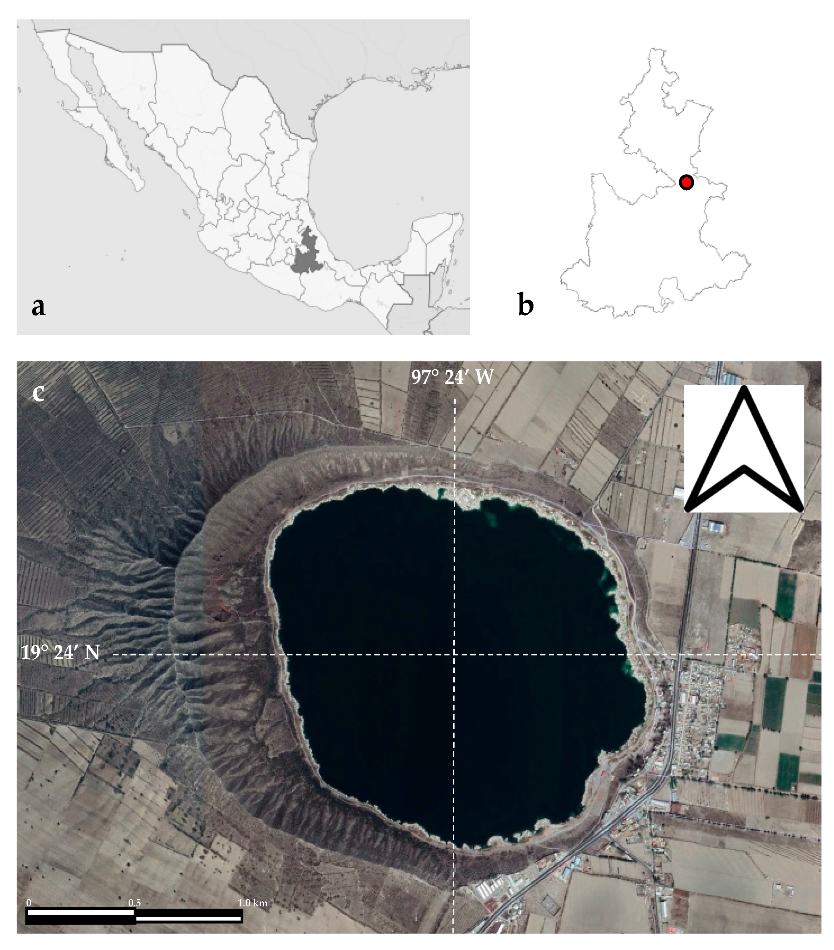
2.1. Study Area
2.2. Field Sampling
2.3. Statistical Analysis
3. Results
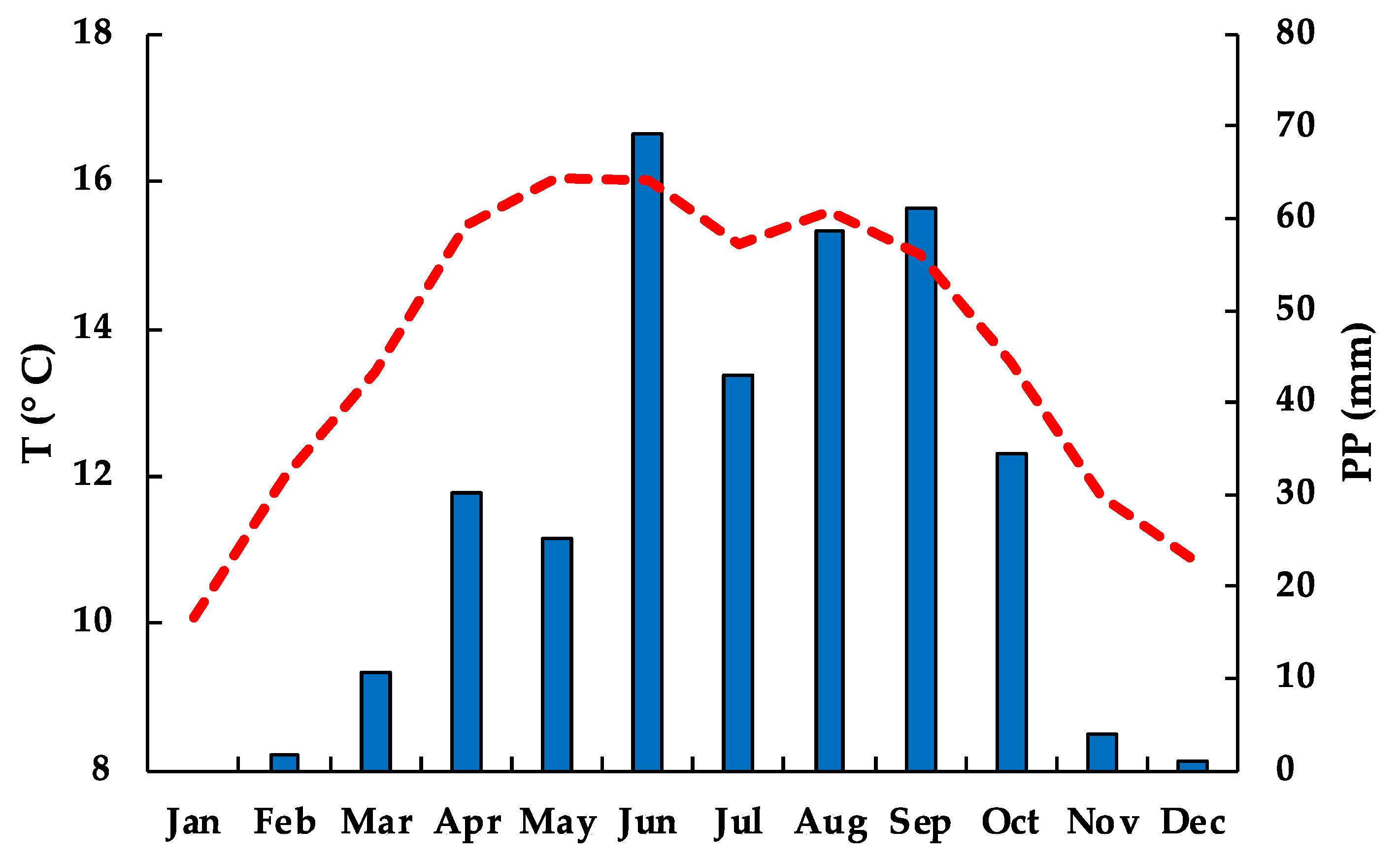
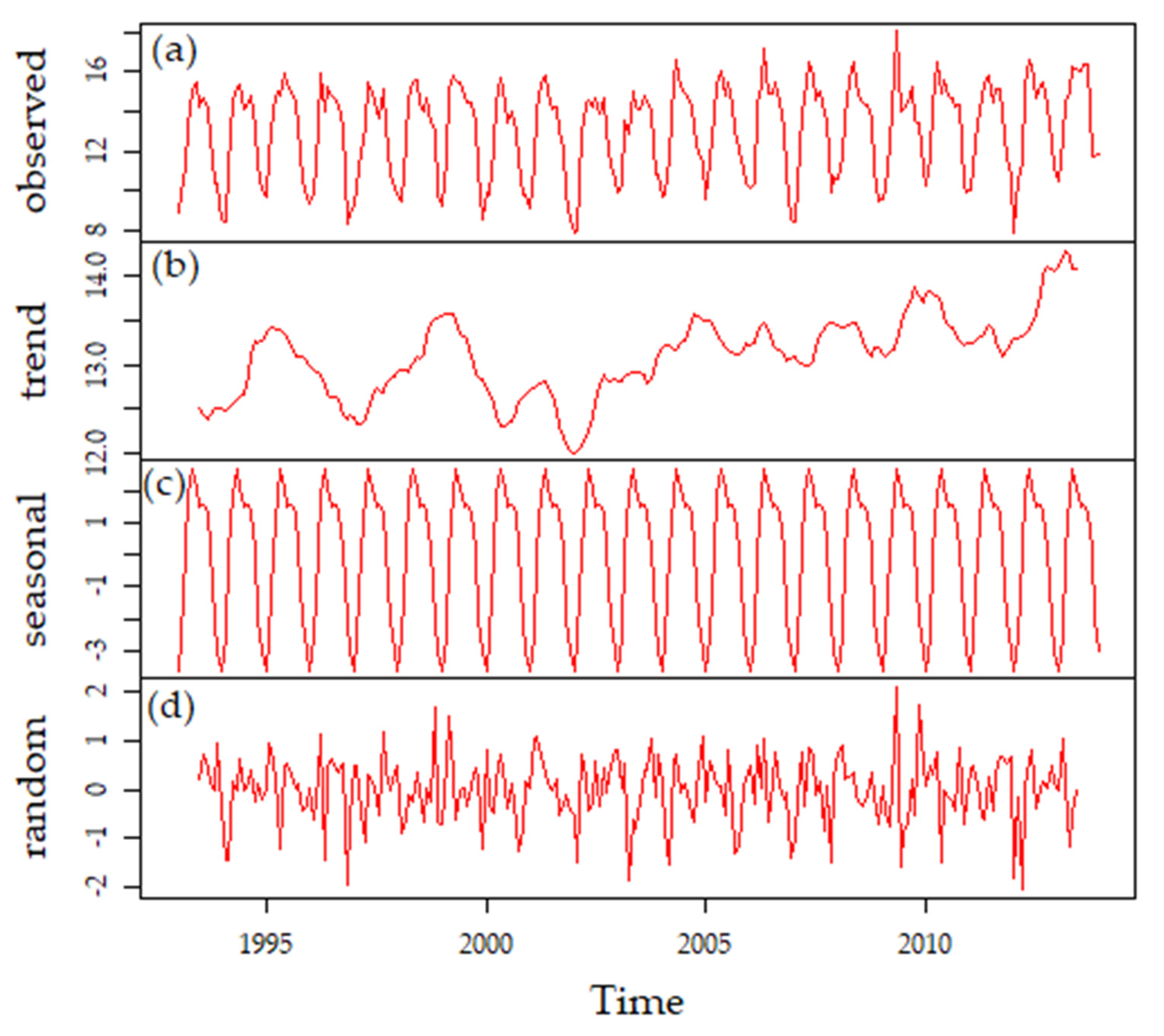
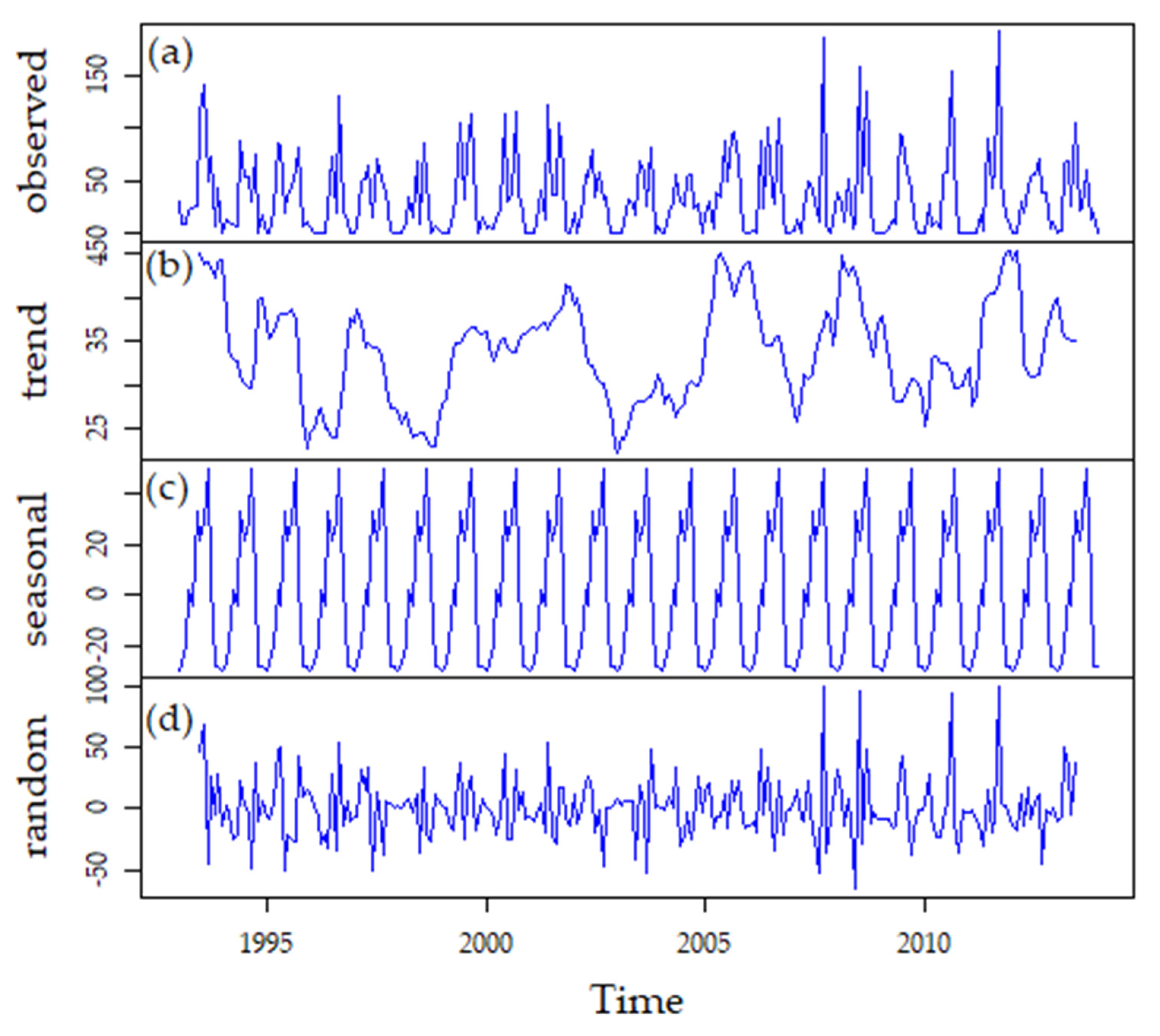
3.1. Climate
3.2. The Aquatic Environment
3.3. The Planktonic Community
3.3.1. The Phytoplankton
3.3.2. The Zooplankton
3.3.3. Long-Term Patterns, Correlations, and Trends
4. Discussion
5. Conclusions
Author Contributions
Funding
Institutional Review Board Statement
Informed Consent Statement
Data Availability Statement
Acknowledgments
Conflicts of Interest
References
- Lewis, S.L.; Maslin, M.A. Defining the Anthropocene. Nature 2015, 519, 171–180. [Google Scholar] [CrossRef] [PubMed]
- Smol, J.P. Under the radar: Long-term perspectives on ecological changes in lakes. Proc. R. Soc. B Biol. Sci. 2019, 286, 20190834. [Google Scholar] [CrossRef] [PubMed]
- Heino, J.; Alahuhta, J.; Bini, L.M.; Cai, Y.; Heiskanen, A.; Hellsten, S.; Kortelainen, P.; Kotamäki, N.; Tolonen, K.T.; Vihervaara, P.; et al. Lakes in the era of global change: Moving beyond single-lake thinking in maintaining biodiversity and ecosystem services. Biol. Rev. 2021, 96, 89–106. [Google Scholar] [CrossRef] [PubMed]
- Luoto, T.P.; Nevalainen, L. Solar and atmospheric forcing on mountain lakes. Sci. Total Environ. 2016, 566–567, 168–174. [Google Scholar] [CrossRef]
- Williamson, C.E.; Dodds, W.; Kratz, T.K.; Palmer, M.A. Lakes and streams as sentinels of environmental change in terrestrial and atmospheric processes. Front. Ecol. Environ. 2008, 6, 247–254. [Google Scholar] [CrossRef]
- Williamson, C.E.; Saros, J.E.; Vincent, W.F.; Smol, J.P. Lakes and reservoirs as sentinels, integrators, and regulators of climate change. Limnol. Oceanogr. 2009, 54, 2273–2282. [Google Scholar] [CrossRef]
- Adrian, R.; O’Reilly, C.M.; Zagarese, H.; Baines, S.B.; Hessen, D.O.; Keller, W.; Livingstone, D.M.; Sommaruga, R.; Straile, D.; Van Donk, E.; et al. Lakes as sentinels of climate change. Limnol. Oceanogr. 2009, 54, 2283–2297. [Google Scholar] [CrossRef]
- Tranvik, L.J.; Downing, J.A.; Cotner, J.B.; Loiselle, S.A.; Striegl, R.G.; Ballatore, T.J.; Dillon, P.; Finlay, K.; Fortino, K.; Knoll, L.B.; et al. Lakes and reservoirs as regulators of carbon cycling and climate. Limnol. Oceanogr. 2009, 54, 2298–2314. [Google Scholar] [CrossRef]
- Woolway, R.I.; Kraemer, B.M.; Lenters, J.D.; Merchant, C.J.; O’Reilly, C.M.; Sharma, S. Global lake responses to climate change. Nat. Rev. Earth Environ. 2020, 1, 388–403. [Google Scholar] [CrossRef]
- Gomes, A.M.D.A.; Marinho, M.M.; Berjante Mesquita, M.C.; Prestes, A.C.C.; Lürling, M.; Azevedo, S.M.F.O. Warming and eutrophication effects on the phytoplankton communities of two tropical water systems of different trophic states: An experimental approach. Lakes Reserv. Sci. Policy Manag. Sustain. Use 2020, 25, 275–282. [Google Scholar] [CrossRef]
- Saulnier-Talbot, É.; Gregory-Eaves, I.; Simpson, K.G.; Efitre, J.; Nowlan, T.E.; Taranu, Z.E.; Chapman, L.J. Small Changes in Climate Can Profoundly Alter the Dynamics and Ecosystem Services of Tropical Crater Lakes. PLoS ONE 2014, 9, e86561. [Google Scholar] [CrossRef] [PubMed]
- Burnett, A.P.; Soreghan, M.J.; Scholz, C.A.; Brown, E.T. Tropical East African climate change and its relation to global climate: A record from Lake Tanganyika, Tropical East Africa, over the past 90+ kyr. Palaeogeogr. Palaeoclimatol. Palaeoecol. 2011, 303, 155–167. [Google Scholar] [CrossRef]
- Scholz, C.A.; King, J.W.; Ellis, G.S.; Swart, P.K.; Stager, J.C.; Colman, S.M. Paleolimnology of Lake Tanganyika, East Africa, over the past 100 kyr. J. Paleolimnol. 2003, 30, 139–150. [Google Scholar] [CrossRef]
- Livingstone, D.A. Global Climate Change Strikes a Tropical Lake. Science 2003, 301, 468–469. [Google Scholar] [CrossRef] [PubMed]
- Plisnier, P.-D.; Nshombo, M.; Mgana, H.; Ntakimazi, G. Monitoring climate change and anthropogenic pressure at Lake Tanganyika. J. Great Lakes Res. 2018, 44, 1194–1208. [Google Scholar] [CrossRef]
- Caballero, M.; Vázquez, G.; Lozano-García, S.; Rodríguez, A.; Sosa-Nájera, S.; Ruiz-Fernández, A.C.; Ortega, B. Present Limnological Conditions and Recent (ca. 340 yr) Palaeolimnology of a Tropical Lake in the Sierra de Los Tuxtlas, Eastern Mexico. J. Paleolimnol. 2006, 35, 83–97. [Google Scholar] [CrossRef]
- Caballero, M.; Mora, L.; Muñoz, E.; Escolero, O.; Bonifaz, R.; Ruiz, C.; Prado, B. Anthropogenic influence on the sediment chemistry and diatom assemblages of Balamtetik Lake, Chiapas, Mexico. Environ. Sci. Pollut. Res. 2020, 27, 15935–15943. [Google Scholar] [CrossRef]
- Lozano-García, S.; Figueroa-Rangel, B.; Sosa-Nájera, S.; Caballero, M.; Noren, A.J.; Metcalfe, S.E.; Tellez-Valdés, O.; Ortega-Guerrero, B. Climatic and anthropogenic influences on vegetation changes during the last 5000 years in a seasonal dry tropical forest at the northern limits of the Neotropics. Holocene 2021, 31, 802–813. [Google Scholar] [CrossRef]
- Rodríguez-Ramírez, A.; Caballero, M.; Roy, P.; Ortega, B.; Vázquez-Castro, G.; Lozano-García, S. Climatic variability and human impact during the last 2000 years in western Mesoamerica: Evidence of late Classic (AD 600–900) and Little Ice Age drought events. Clim. Past 2015, 11, 1239–1248. [Google Scholar] [CrossRef]
- Alcocer, J.; Delgado, C.N.; Sommaruga, R. Photoprotective compounds in zooplankton of two adjacent tropical high mountain lakes with contrasting underwater light climate and fish occurrence. J. Plankton Res. 2020, 42, 105–118. [Google Scholar] [CrossRef]
- García, E. Modoficaciones al Sistema de Clasificación Climática de Köppen (Para Adaptarlo a las Condiciones de la República Mexicana); Cuarta edi; Offset Larios: Ciudad de México, México, 1988. [Google Scholar]
- Adame, M.F.; Alcocer, J.; Escobar, E. Size-fractionated phytoplankton biomass and its implications for the dynamics of an oligotrophic tropical lake. Freshw. Biol. 2008, 53, 22–31. [Google Scholar] [CrossRef]
- Silva-Aguilera, R.; Escolero, O.; Alcocer, J. Recent Climate of Serdán-Oriental Basin. In Lake Alchichica Limnology. The Uniqueness of a Tropical Maar Lake; Javier, A., Ed.; Springer: Cham, Switzerland, 2022; pp. 51–91. ISBN 978-3-030-79095-0. [Google Scholar]
- Filonov, A.; Tereshchenko, I.; Barba-López, M.R.; Alcocer, J.; Ladah, L. Meteorological regime, local climate, and hydrodynamics of Lake Alchichica. In Lake Alchichica Limnology: The Uniqueness of a Tropical Maar Lake; Alcocer, J., Ed.; Springer: Cham, Switzerland, 2022; ISBN 978-3-030-79095-0. [Google Scholar]
- Armienta, M.A.; Vilaclara, G.; De la Cruz-Reyna, S.; Ramos, S.; Ceniceros, N.; Cruz, O.; Aguayo, A.; Arcega-Cabrera, F. Water chemistry of lakes related to active and inactive Mexican volcanoes. J. Volcanol. Geotherm. Res. 2008, 178, 249–258. [Google Scholar] [CrossRef]
- Alcocer, J.; Lugo, A.; Escobar, E.; Sànchez, M.R.; Vilaclara, G. Water column stratification and its implications in the tropical warm monomictic Lake Alchichica, Puebla, Mexico. Verhandlungen Int. Verein Limnol. 2000, 27, 3166–3169. [Google Scholar] [CrossRef]
- Ramírez-Olvera, M.A.; Alcocer, J.; Merino-Ibarra, M.; Lugo, A. Nutrient limitation in a tropical saline lake: A microcosm experiment. Hydrobiologia 2009, 626, 5–13. [Google Scholar] [CrossRef]
- Searcy, J.K.; Hardison, C.H. Double-Mass Curves (No. 1541). Manual of Hydrology: Part 1. General Surface-Water Techniques. Water-Supply Paper; USGPO: Washington, DC, USA, 1960. [Google Scholar]
- Arar, E.J.; Collins, G.B. Method 445.0 In Vitro Determination of Chlorophyll and Pheophytin a in Marine and Freshwater Algae by Fluorescence; U.S. Environmental Protection Agency: Cincinnati, OH, USA, 1997.
- Utermöhl, H. Zur Vervollkomung der quantitativen Phytoplankton-Methodik. Mitt. Int. Ver. Limnol. 1958, 9, 1–38. [Google Scholar]
- Olenina, I.; Hajdu, S.; Edler, L.; Andersson, A.; Wasmund, N.; Busch, S.; Göbel, J.; Gromisz, S.; Huseby, S.; Huttunen, M.; et al. Biovolumes and Size-Classes of Phytoplankton in the Baltic Sea; No. 106.; HELCOM: Helsinki, Finland, 2006; ISBN 0357-2994. [Google Scholar]
- Comas-González, A. Las Chlorococcales Dulceacuícolas de Cuba [The Freshwater Chlorococcids of Cuba]; Bibliotheca Phycologica: Stuttgart, Berlin, 1996. [Google Scholar]
- Krammer, K. Large-Bertalot Suesswasserflora von Mitteleuropa. Band 2/3: Bacillariophyceae, 3. Teil: Bacillariaceae (Centrales, Fragilariaceae, Eunotionaceae); Springer Spektrum: Stuttgart, Germany, 1991. [Google Scholar]
- Komárek, J.; Fott, B. Chlorophyceae (Gruenalgen), Ordnung Chlorococcales. (Huber-Pestalozzi, G. Das Phytoplankton des Siuesswassers. 7. Teil, 1. Haelfte). In Die Binnengewaesser; Huber-Pestalozzi, Ed.; Schweizerbart‘sche Buchhandlung: Stuttgart, Germany, 1983. [Google Scholar]
- Lehtimäki, J.; Lyra, C.; Suomalainen, S.; Sundman, P.; Rouhiainen, L.; Paulin, L.; Salkinoja-Salonen, M.; Sivonen, K. Characterization of Nodularia strains, cyanobacteria from brackish waters, by genotypic and phenotypic methods. Int. J. Syst. Evol. Microbiol. 2000, 50, 1043–1053. [Google Scholar] [CrossRef] [PubMed]
- Oliva, M.G.; Lugo, A.; Alcocer, J.; Cantoral-Uriza, E.A. Cyclotella alchichicana sp. nov. from a saline mexican lake. Diatom Res. 2006, 21, 81–89. [Google Scholar] [CrossRef]
- Oliva, M.G.; Lugo, A.; Alcocer, J.; Cantoral-Uriza, E.A. Morphological study of Cyclotella choctawhatcheeana prasad (Stephanodiscaceae) from a saline Mexican lake. Saline Syst. 2008, 4, 1–9. [Google Scholar] [CrossRef]
- Rushfnrth, S.R.; Johansen, J.R. The inland Chaetoceros (Bacillariophyceae) species of North America. J. Phycol. 1986, 22, 441–448. [Google Scholar] [CrossRef]
- Tavera, R.; Komárek, J. Cyanoprokariotes in the volcanic lake of Alchichica, Puebla State, Mexico. Die Binnengewaesser 1983, 83, 511. [Google Scholar]
- Wehr, J.D.; Sheath, R.G.; Kociolek, J.P. Freshwater Algae of North America, 2nd ed.; Academic Press: Cambridge, MA, USA, 2015. [Google Scholar]
- Dusart, B.H.; Defayane, D. Introduction to the Copepoda; SPB: Amsterdam, The Netherlands, 1995. [Google Scholar]
- Cassie, R.M. Sampling and Statistics. In A Manual on Methods for the Assessment of Secondary Productivity in Freshwaters.; Edmonson, W.T., Winberg, G.G., Eds.; Blackwell: Oxford and Edinburgh, UK, 1971; pp. 174–209. [Google Scholar]
- Koste, W. Rotatoria: D. Rädertiere Mitteleuropas e. Bestimmungswerk; Überordnung Monogononta, 1st ed.; Gebrüder Borntraeger Verlag: Berlin, Germany, 1978. [Google Scholar]
- Mills, S.; Alcántara-Rodríguez, J.A.; Ciros-Pérez, J.; Gómez, A.; Hagiwara, A.; Galindo, K.H.; Jersabek, C.D.; Malekzadeh-Viayeh, R.; Leasi, F.; Lee, J.S.; et al. Fifteen species in one: Deciphering the Brachionus plicatilis species complex (Rotifera, Monogononta) through DNA taxonomy. Hydrobiologia 2017, 796, 39–58. [Google Scholar] [CrossRef]
- Montiel-Martínez, A.; Ciros-Pérez, J.; Ortega-Mayagoitia, E.; Elías-Gutiérrez, M. Morphological, ecological, reproductive and molecular evidence for Leptodiaptomus garciai (Osorio-Tafall 1942) as a valid endemic species. J. Plankton Res. 2008, 30, 1079–1093. [Google Scholar] [CrossRef]
- Ciros-Pérez, J.; Ortega-Mayagoitia, E.; Alcocer, J. The role of ecophysiological and behavioral traits in structuring the zooplankton assemblage in a deep, oligotrophic, tropical lake. Limnol. Oceanogr. 2015, 60, 2158–2172. [Google Scholar] [CrossRef]
- Ruttner-Kolisko, A. Suggestions for biomass calculation of plankton rotifers. Arch. Hydrobiol. Beih. Ergebn. Limnol. 1977, 8, 71–76. [Google Scholar]
- McCauley, E. The estimation of the abundance and biomass of zooplankton in samples. In A Manual on Methods for the Assessment of Secondary Productivity in Fresh Waters; Downing, J., Rigler, F.H., Eds.; Blackwell Scientific Pub: Norkfold, England, 1984; pp. 228–265. [Google Scholar]
- R Core Team. R: A Language and Environment for Statistical Computing; R Core Team: Vienna, Austria, 2021. [Google Scholar]
- Laboratory, N.P.S. Climate Indices: Monthly Atmospheric and Ocean Time-Series. Available online: https://psl.noaa.gov/data/climateindices/list/ (accessed on 28 February 2022).
- Hammer, Ø.; Harper, D.A.T.; Ryan, D. PAST: Paleontological Statistics Software Package for Education and Data Analysis. Paleontol. Electron. 2001, 4, 9. [Google Scholar]
- Cuevas-Lara, J.D.; Alcocer, J.; Oseguera, L.A.; Quiroz-Martínez, B. Dinámica a largo plazo (1999–2014) de la productividad primaria fitoplanctónica en el Lago Alchichica. In Estado Actual del Conocimiento del Ciclo del Carbono y Sus Interacciones en México: Síntesis a 2016; Paz, F., Torres, R., Eds.; Programa Mexicano del Carbono en colaboración con la Universidad Autónoma del Estado de Hidalgo: Texcoco, Mexico, 2016; pp. 280–286. ISBN 978-607-96490-4-3. [Google Scholar]
- Lewis, W.M. A revised classification of lakes based on mixing. Can. J. Fish. Aquat. Sci. 1983, 40, 1779–1787. [Google Scholar] [CrossRef]
- Alcocer, J. (Ed.) Lake Alchichica Limnology—The Uniqueness of a Tropical Maar Lake.; Springer: Cham, Switzerland, 2022; ISBN 978-3-030-79095-0. [Google Scholar]
- Alcocer, J.; Lugo, A. Effects of El Niño on the dynamics of Lake Alchichica, central Mexico. Geofísica Int. 2003, 42, 523–528. [Google Scholar]
- Bravo-Cabrera, J.L.; Azpra-Romero, E.; Zarraluqui-Such, V.; Gay-Garcia, C. Effects of El Niño in Mexico during rainy and dry seasons: An extended treatment. Atmósfera 2017, 30, 221–232. [Google Scholar] [CrossRef]
- Park, J.; Byrne, R.; Böhnel, H. The combined influence of Pacific decadal oscillation and Atlantic multidecadal oscillation on central Mexico since the early 1600s. Earth Planet. Sci. Lett. 2017, 464, 1–9. [Google Scholar] [CrossRef]
- Pavia, E.G.; Graef, F.; Reyes, J. PDO–ENSO Effects in the Climate of Mexico. J. Clim. 2006, 19, 6433–6438. [Google Scholar] [CrossRef]
- Trenberth, K.E. Recent observed interdecadal climate changes in the Northern Hemisphere. Bull. Am. Meteorol. Soc. 1990, 71, 988–993. [Google Scholar] [CrossRef]
- Graham, N.E. Decadal-scale climate variability in the 1970’s and 1980’s: Observations and model results. Clim. Dyn. 1994, 10, 135–159. [Google Scholar] [CrossRef]
- Latif, M.; Barnett, T.P. Causes of decadal climate variability over the North Pacific and North America. Science 1994, 266, 634–637. [Google Scholar] [CrossRef] [PubMed]
- Minobe, S. A 50-70 year climatic oscillation over the North Pacific and North America. Geophys. Res. Lett. 1997, 24, 683–686. [Google Scholar] [CrossRef]
- Zhang, Y.; Wallace, J.M.; Battisti, D.S. ENSO-like interdecadal variability: 1900–93. J. Clim. 1997, 10, 1004–1020. [Google Scholar] [CrossRef]
- IPCC. Intergovernmental Panel on Climate Change. In The Physical Science Basis. Contribution of Working Group I to the Fifth Assessment Report of the Intergovernmental Panel on Climate Change; Cambridge University Press: Cambridge, UK; New York, NY, USA, 2013. [Google Scholar]
- Vadadi-Fülöp, C.; Sipkay, C.; Mészáros, G.; Hufnagel, L. Climate change and freshwater zooplankton: What does it boil down to? Aquat. Ecol. 2012, 46, 501–519. [Google Scholar] [CrossRef][Green Version]
- Michelutti, N.; Wolfe, A.P.; Cooke, C.A.; Hobbs, W.O.; Vuille, M.; Smol, J.P. Climate change forces new ecological states in tropical Andean lakes. PLoS ONE 2015, 10, e0115338. [Google Scholar] [CrossRef]
- Carter, J.L.; Schindler, D.E.; Francis, T.B. Effects of climate change on zooplankton community interactions in an Alaskan lake. Clim. Chang. Responses 2017, 4, 3. [Google Scholar] [CrossRef]
- Lewis, W.M. Phytoplankton Succession in Lake Valencia, Venezuela. Hydrobiologia 1986, 138, 189–203. [Google Scholar] [CrossRef]
- Richerson, P.J.; Neale, P.J.; Wurtsbaugh, W.; Alfaro, T.R.; Vincent, W. Patterns of temporal variation in Lake Titicaca. A high altitude tropical lake. I. Background, physical and chemical processes, and primary production. Hydrobiologia 1986, 138, 205–220. [Google Scholar] [CrossRef]
- Paul, C.; Sommer, U.; Matthiessen, B. Composition and dominance of edible and inedible phytoplankton predict responses of Baltic Sea summer communities to elevated temperature and CO2. Microorganisms 2021, 9, 2294. [Google Scholar] [CrossRef] [PubMed]
- Bell, T. The ecological consequences of unpalatable prey: Phytoplankton response to nutrient and predator additions. Oikos 2002, 99, 59–68. [Google Scholar] [CrossRef]
- Catalan, J.; Pla-Rabés, S.; Wolfe, A.P.; Smol, J.P.; Rühland, K.M.; Anderson, N.J.; Kopáček, J.; Stuchlík, E.; Schmidt, R.; Koinig, K.A.; et al. Global change revealed by palaeolimnological records from remote lakes: A review. J. Paleolimnol. 2013, 49, 513–535. [Google Scholar] [CrossRef]
- Silva-Aguilera, R.A.; Vilaclara, G.; Armienta, M.A.; Escolero, O. Hydrogeology and hydrochemistry of the Serdán-Oriental Basin and the Lake Alchichica. In Lake Alchichica Limnology—The Uniqueness of a Tropical Maar Lake; Alcocer, J., Ed.; Springer: Cham, Switzerland, 2022; ISBN 978-3-030-79095-0. [Google Scholar]
- González Contreras, C.G.; Alcocer, J.; Oseguera, L.A. Phytoplankton chlorophyll a in the tropical deep Alchichica: A long-term record (1999–2010). Hidrobiológica 2015, 25, 347–356. [Google Scholar]
- Ardiles, V.; Alcocer, J.; Vilaclara, G.; Oseguera, L.A.; Velasco, L. Diatom fluxes in a tropical, oligotrophic lake dominated by large-sized phytoplankton. Hydrobiologia 2012, 679, 77–90. [Google Scholar] [CrossRef]
- Escobar, E.; Alcocer, J. Lake foof webs. In Lake Alchichica Limnology—The Uniqueness of a Tropical Maar Lake; Alcocer, J., Ed.; Springer: Cham, Switzerland, 2022; ISBN 978-3-030-79095-0. [Google Scholar]
- Oliva, M.G.; Lugo, A.; Alcocer, J.; Peralata, L.; Oseguera, L.A. Planktonic bloom-forming Nodularia in the saline Lake Alchichica, Mexico. Nat. Resour. Environ. Issues 2009, 15, 121–126. [Google Scholar]
- Ortega-Mayagoitia, E.; Ciros-Pérez, J.; Sánchez-Martínez, M. A story of famine in the pelagic realm: Temporal and spatial patterns of food limitation in rotifers from an oligotrophic tropical lake. J. Plankton Res. 2011, 33, 1574–1585. [Google Scholar] [CrossRef]
- Vilaclara, G.; Oliva-Martinez, M.G.; Macek, M.; Ortega-Mayagoitia, E.; Alcantara-Hernandez, R.J.; Lopez-Vazquez, C. A unique community for an oligotrophic lake. In Lake Alchichica Limnology—The Uniqueness of a Tropical Maar Lake.; Alcocer, J., Ed.; Springer: Cham, Switzerland, 2022; ISBN 978-3-030-79095-0. [Google Scholar]
- Alcocer, J.; Ruiz-Fernández, A.C.; Escobar, E.; Pérez-Bernal, L.H.; Oseguera, L.A.; Ardiles-Gloria, V. Deposition, burial and sequestration of carbon in an oligotrophic, tropical lake. J. Limnol. 2014, 73, 223–235. [Google Scholar] [CrossRef]
- Oseguera, L.A.; Alcocer, J.; Vilaclara, G. Relative importance of dust inputs and aquatic biological production as sources of lake sediments in an oligotrophic lake in a semi-arid area. Earth Surf. Process. Landforms 2011, 36, 419–426. [Google Scholar] [CrossRef]
- Kondoh, M. Foraging Adaptation and the relationship between food-web complexity and stability. Science 2003, 299, 1388–1391. [Google Scholar] [CrossRef]
- Bernát, G.; Boross, N.; Somogyi, B.; Vörös, L.; G-Tóth, L.; Boros, G. Oligotrophication of Lake Balaton over a 20-year period and its implications for the relationship between phytoplankton and zooplankton biomass. Hydrobiologia 2020, 847, 3999–4013. [Google Scholar] [CrossRef]
- Fernández, R.; Alcocer, J.; Lugo, A.; Oseguera, L.A.; Guadarrama-Hernández, S. Seasonal and interannual dynamics of pelagic rotifers in a tropical, saline, deep lake. Diversity 2022, 14, 113. [Google Scholar] [CrossRef]
- Ortega-Mayagoitia, E.; Alcántara-Rodríguez, J.A.; Lugo-Vázquez, A.; Montiel-Martínez, A.; Ciros-Pérez, J. The joys and challenges of living in a saline, oligotrophic, warm monomictic lake. In Lake Alchichica Limnology: The Uniqueness of a Tropical Maar Lake; Alcocer, J., Ed.; Springer: Cham, Switzerland, 2022; ISBN 978-3-030-79095-0. [Google Scholar]
- Ortega-Mayagoitia, E.; Hernández-Martínez, O.; Ciros-Pérez, J. Phenotypic plasticity of life-history traits of a calanoid copepod in a tropical lake: Is the magnitude of thermal plasticity related to thermal variability? PLoS ONE 2018, 13, e0196496. [Google Scholar] [CrossRef] [PubMed]
- IPCC Summary for Policymakers. Climate Change 2021: The Physical Science Basis. Contribution of Working Group I to the Sixth Assessment Report of the Intergovernmental Panel on Climate Change; Masson-Delmotte, V., Zhai, P., Pirani, A., Connors, S.L., Péan, C., Berger, S., Caud, N., Chen, Y., Goldfarb, L., Gomis, M.I., et al., Eds.; Cambridge University Press: Cambridge, UK, 2021. [Google Scholar]
- Sarmento, H.; Amado, A.M.; Descy, J.P. Climate change in tropical fresh waters (comment on the paper “Plankton dynamics under different climatic conditions in space and time” by de Senerpont Domis et al.). Freshw. Biol. 2013, 58, 2208–2210. [Google Scholar] [CrossRef]


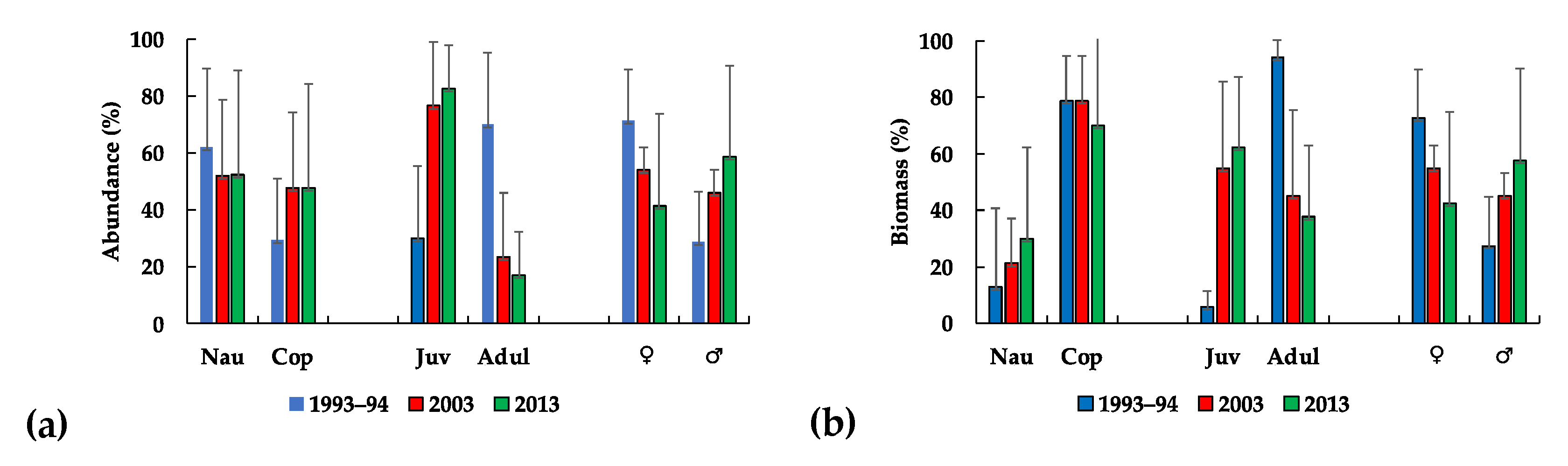
 : females,
  : males).
: females, : males).
: males).
: females, : males).

| Variable | S | Z | p | Trend | |
|---|---|---|---|---|---|
| Phytoplankton | C. alchichicana abundance and biomass | 284 | 3.8547 | 0.00001 | Increase |
| Chaetoceros elmorei abundance and biomass | −161 | 2.1884 | 0.028 | Decrease | |
| C. choctawhatcheeana abundance and biomass | −255 | 3.46 | 0.005 | Decrease | |
| O. submarina abundance and biomass | −202 | 2.7545 | 0.0058 | Decrease | |
| Total phytoplankton abundance and biomass | 274 | 3.7185 | 0.0002 | Increase | |
| Zooplankton | L. garciai female abundance | −272 | 3.7009 | 0.0002 | Decrease |
| L. garciai male abundance | −216 | 2.935 | 0.0033 | Decrease | |
| Total L. garciai adults | −265 | 3.6023 | 0.0003 | Decrease | |
| Total copepods abundance | −144 | 1.4608 | 0.049 | Decrease | |
| L. garciai female biomass | −274 | 3.7261 | 0.0001 | Decrease | |
| L. garciai male biomass | −321 | 3.0032 | 0.0026 | Decrease | |
| Adult copepods biomass | −266 | 3.6189 | 0.0029 | Decrease | |
| Total copepods biomass | −226 | 3.0717 | 0.0021 | Decrease |
Publisher’s Note: MDPI stays neutral with regard to jurisdictional claims in published maps and institutional affiliations. |
© 2022 by the authors. Licensee MDPI, Basel, Switzerland. This article is an open access article distributed under the terms and conditions of the Creative Commons Attribution (CC BY) license (https://creativecommons.org/licenses/by/4.0/).
Share and Cite
Alcocer, J.; Lugo, A.; Fernández, R.; Vilaclara, G.; Oliva, M.G.; Oseguera, L.A.; Silva-Aguilera, R.A.; Escolero, Ó. 20 Years of Global Change on the Limnology and Plankton of a Tropical, High-Altitude Lake. Diversity 2022, 14, 190. https://doi.org/10.3390/d14030190
Alcocer J, Lugo A, Fernández R, Vilaclara G, Oliva MG, Oseguera LA, Silva-Aguilera RA, Escolero Ó. 20 Years of Global Change on the Limnology and Plankton of a Tropical, High-Altitude Lake. Diversity. 2022; 14(3):190. https://doi.org/10.3390/d14030190
Chicago/Turabian StyleAlcocer, Javier, Alfonso Lugo, Rocío Fernández, Gloria Vilaclara, María Guadalupe Oliva, Luis A. Oseguera, Raúl A. Silva-Aguilera, and Óscar Escolero. 2022. "20 Years of Global Change on the Limnology and Plankton of a Tropical, High-Altitude Lake" Diversity 14, no. 3: 190. https://doi.org/10.3390/d14030190
APA StyleAlcocer, J., Lugo, A., Fernández, R., Vilaclara, G., Oliva, M. G., Oseguera, L. A., Silva-Aguilera, R. A., & Escolero, Ó. (2022). 20 Years of Global Change on the Limnology and Plankton of a Tropical, High-Altitude Lake. Diversity, 14(3), 190. https://doi.org/10.3390/d14030190