
Underwater Video as a Tool to Quantify Fish Density in Complex Coastal Habitats

 ,
,
Abstract
:1. Introduction
2. Materials and Methods
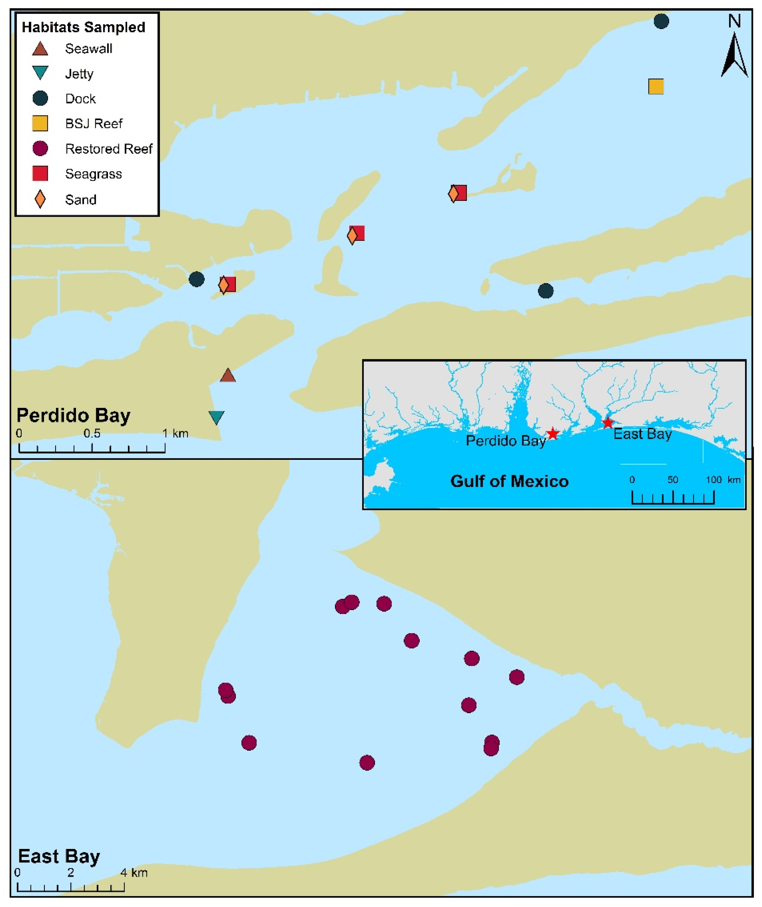
2.1. Study Sites
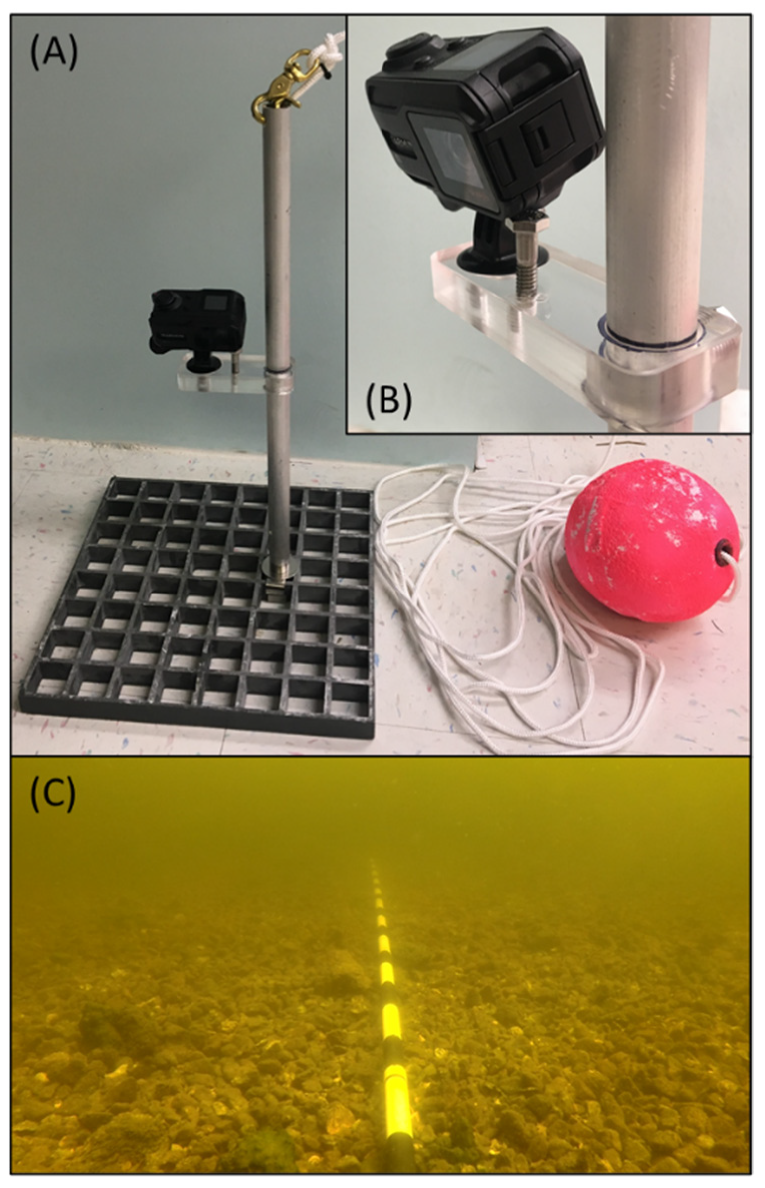
2.2. Field Sampling
2.3. Video Data Processing
2.4. Data Analysis
3. Results
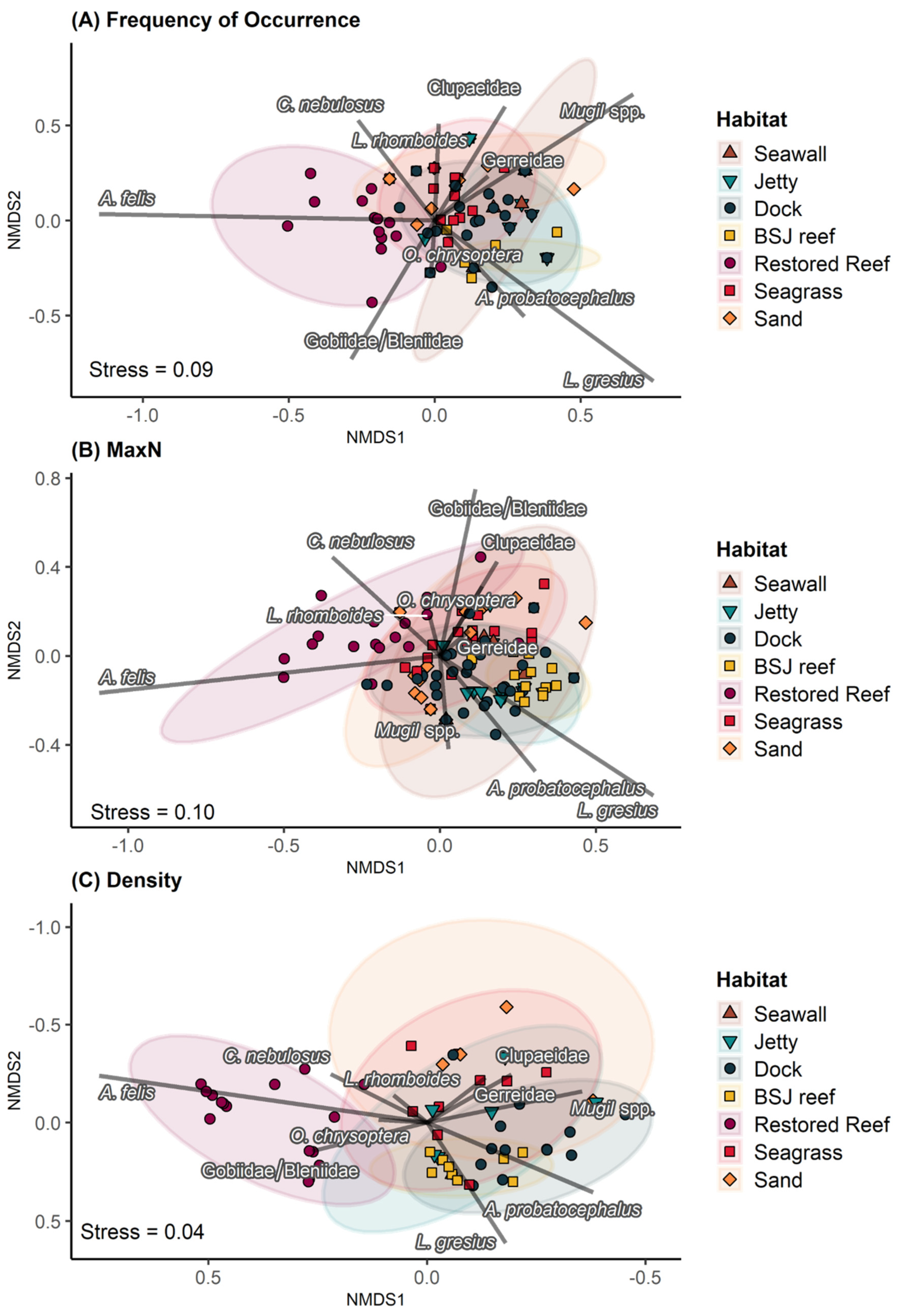
3.1. Assemblage Composition
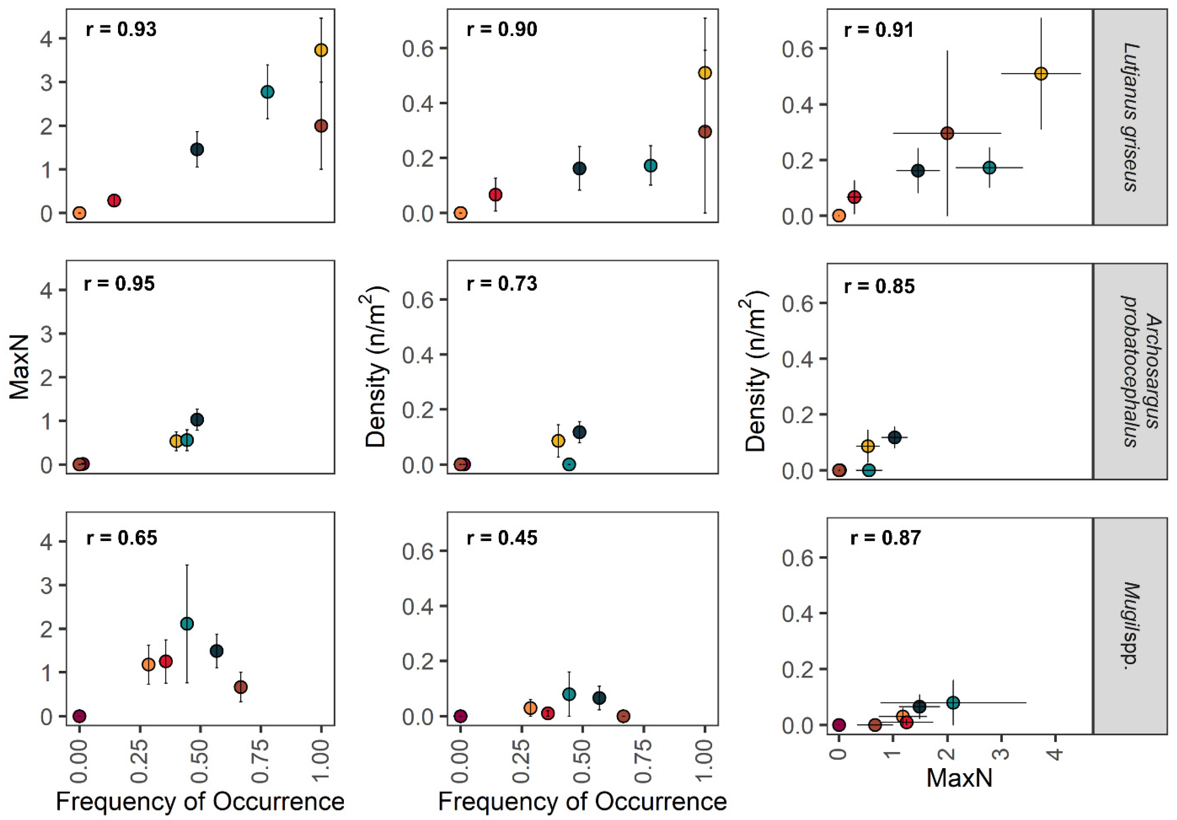
3.2. Comparison of Metrics for Common Taxa
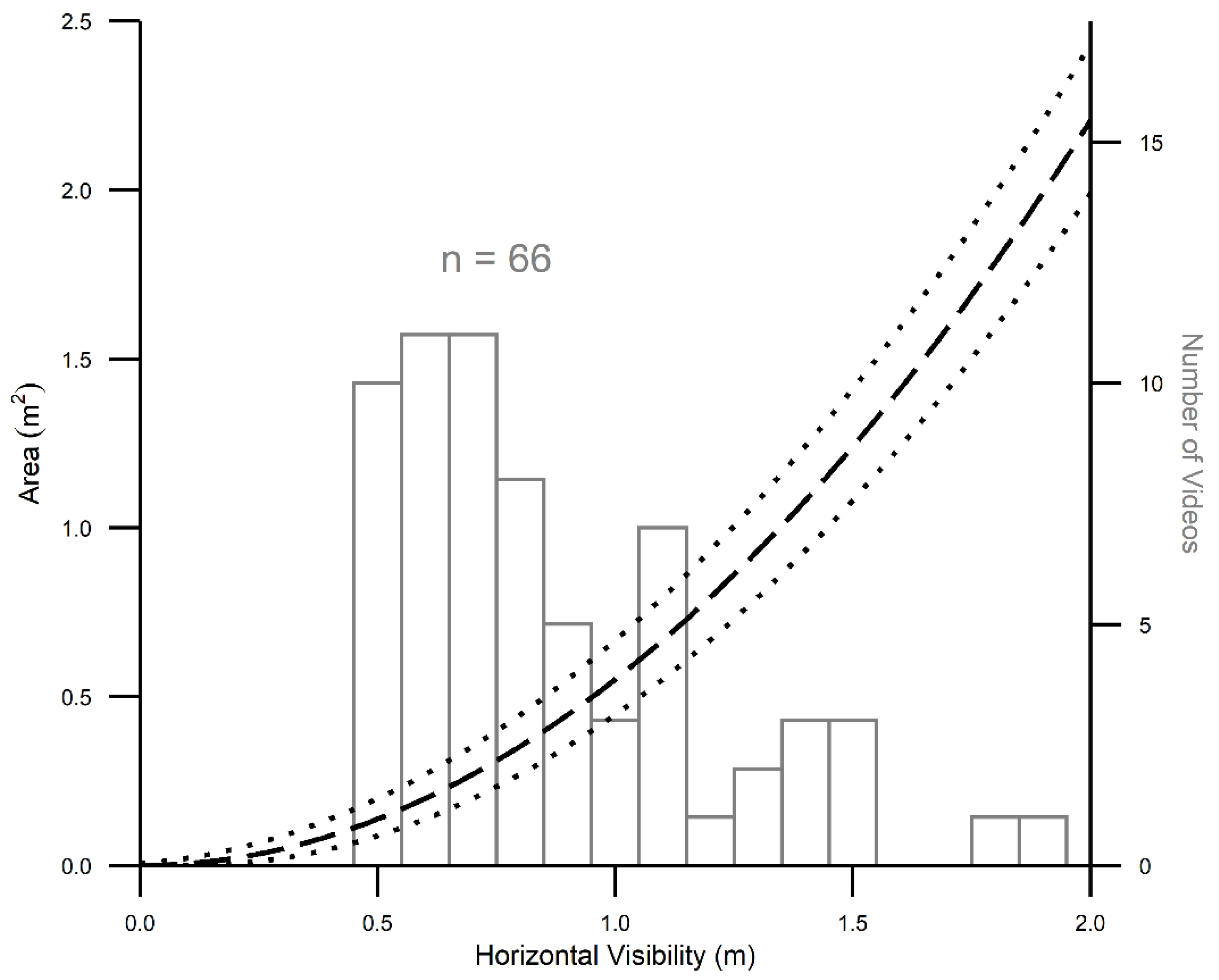
3.3. Precision in Estimating Area Sampled
4. Discussion
4.1. Comparison of Metrics for Quantifying Fish Assemblages
4.2. Challenges and Solutions
5. Conclusions
Supplementary Materials
Author Contributions
Funding
Institutional Review Board Statement
Informed Consent Statement
Data Availability Statement
Acknowledgments
Conflicts of Interest
References
- Hanski, I. Habitat Loss, the Dynamics of Biodiversity, and a Perspective on Conservation. Ambio 2011, 40, 248–255. [Google Scholar] [CrossRef] [Green Version]
- Powers, R.P.; Jetz, W. Global habitat loss and extinction risk of terrestrial vertebrates under future land-use-change scenarios. Nat. Clim. Chang. 2019, 9, 323–329. [Google Scholar] [CrossRef]
- Zu Ermgassen, P.S.; Spalding, M.D.; Blake, B.; Coen, L.D.; Dumbauld, B.; Geiger, S.; Grabowski, J.H.; Grizzle, R.; Luckenbach, M.; McGraw, K.; et al. Historical ecology with real numbers: Past and present extent and biomass of an imperiled estuarine habitat. Proc. R. Soc. B 2012, 279, 3393–3400. [Google Scholar] [CrossRef] [Green Version]
- Gedan, K.B.; Silliman, B.R.; Bertness, M.D. Centuries of Human-Driven Change in Salt Marsh Ecosystems. Annu. Rev. Mar. Sci. 2009, 1, 117–141. [Google Scholar] [CrossRef] [Green Version]
- Unsworth, R.K.F.; McKenzie, L.J.; Collier, C.J.; Cullen-Unsworth, L.C.; Duarte, C.M.; Eklöf, J.S.; Jarvis, J.C.; Jones, B.L.; Nordlund, L.M. Global challenges for seagrass conservation. Ambio 2019, 48, 801–815. [Google Scholar] [CrossRef] [Green Version]
- Waltham, N.J.; Connolly, R.M. Global extent and distribution of artificial, residential waterways in estuaries. Estuar. Coast. Shelf Sci. 2011, 94, 192–197. [Google Scholar] [CrossRef]
- Gilby, B.L.; Weinstein, M.P.; Baker, R.; Cebrian, J.; Alford, S.B.; Chelsky, A.; Colombano, D.; Connolly, R.M.; Currin, C.A.; Feller, I.C.; et al. Human Actions Alter Tidal Marsh Seascapes and the Provision of Ecosystem Services. Chesap. Sci. 2021, 44, 1628–1636. [Google Scholar] [CrossRef]
- Dafforn, K.A.; Mayer-Pinto, M.; Morris, R.L.; Waltham, N.J. Application of management tools to integrate ecological princi-ples with the design of marine infrastructure. J. Environ. Manag. 2015, 158, 61–73. [Google Scholar] [CrossRef]
- Munsch, S.H.; Cordell, J.R.; Toft, J.D. Effects of shoreline armouring and overwater structures on coastal and estuarine fish: Opportunities for habitat improvement. J. Appl. Ecol. 2017, 54, 1373–1384. [Google Scholar] [CrossRef] [Green Version]
- Sharma, S.; Goff, J.; Cebrian, J.; Ferraro, C. A hybrid shoreline stabilization technique: Impact of modified intertidal reefs on marsh expansion and nekton habitat in the northern Gulf of Mexico. Ecol. Eng. 2016, 90, 352–360. [Google Scholar] [CrossRef]
- Folpp, H.R.; Schilling, H.T.; Clark, G.F.; Lowry, M.B.; Maslen, B.; Gregson, M.; Suthers, I.M. Artificial reefs increase fish abundance in habitat-limited estuaries. J. Appl. Ecol. 2020, 57, 1752–1761. [Google Scholar] [CrossRef]
- Waltham, N.J.; Alcott, C.; Barbeau, M.A.; Cebrian, J.; Connolly, R.M.; Deegan, L.A.; Dodds, K.; Gaines, L.A.G.; Gilby, B.L.; Henderson, C.J.; et al. Tidal Marsh Restoration Optimism in a Changing Climate and Urbanizing Seascape. Estuaries Coasts 2021, 44, 1681–1690. [Google Scholar] [CrossRef]
- Zu Ermgassen, P.S.E.; Grabowski, J.H.; Gair, J.R.; Powers, S. Quantifying fish and mobile invertebrate production from a threatened nursery habitat. J. Appl. Ecol. 2016, 53, 596–606. [Google Scholar] [CrossRef] [Green Version]
- Zu Ermgassen, P.S.; DeAngelis, B.; Gair, J.R.; zu Ermgassen, S.; Baker, R.; Daniels, A.; MacDonald, T.C.; Meckley, K.; Powers, S.; Ribera, M.; et al. Estimating and applying fish and invertebrate density and production enhancement from seagrass, salt marsh edge, and oyster reef nursery habitats in the Gulf of Mexico. Estuaries Coasts 2021, 44, 1588–1603. [Google Scholar] [CrossRef]
- Rozas, L.P.; Minello, T.J. Estimating Densities of Small Fishes and Decapod Crustaceans in Shallow Estuarine Habitats: A Review of Sampling Design with Focus on Gear Selection. Estuaries 1997, 20, 199–213. [Google Scholar] [CrossRef]
- Becker, A.; Cowley, P.D.; Whitfield, A.K. Use of remote underwater video to record littoral habitat use by fish within a temporarily closed South African estuary. J. Exp. Mar. Biol. Ecol. 2010, 391, 161–168. [Google Scholar] [CrossRef]
- Mallet, D.; Pelletier, D. Underwater video techniques for observing coastal marine biodiversity: A review of sixty years of publications (1952–2012). Fish. Res. 2014, 154, 44–62. [Google Scholar] [CrossRef]
- Bradley, M.; Baker, R.; Nagelkerken, I.; Sheaves, M. Context is more important than habitat type in determining use by juvenile fish. Lands. Ecol. 2019, 34, 427–442. [Google Scholar] [CrossRef]
- Schobernd, Z.H.; Bacheler, N.M.; Conn, P.B. Examining the utility of alternative video monitoring metrics for indexing reef fish abundance. Can. J. Fish. Aquat. Sci. 2014, 71, 464–471. [Google Scholar] [CrossRef]
- Baker, R.; Waltham, N. Tethering mobile aquatic organisms to measure predation: A renewed call for caution. J. Exp. Mar. Biol. Ecol. 2020, 523, 151270. [Google Scholar] [CrossRef]
- Bradley, M.; Nagelkerken, I.; Baker, R.; Travers, M.; Sheaves, M. Local environmental context structures animal-habitat asso-ciations across biogeographic regions. Ecosystems 2021, 9, 1–5. [Google Scholar]
- Patterson, W.F.; Tarnecki, J.H.; Addis, D.T.; Barbieri, L.R. Reef fish community structure at natural versus artificial reefs in the northern Gulf of Mexico. Proc. Gulf Carib. Fish. Inst. 2014, 66, 4–8. [Google Scholar]
- Stunz, G.W.; Patterson, W.F.; Powers, S.P.; Cowan, J.H.; Rooker, J.R.; Ahrens, R.A.; Boswell, K.; Carleton, L.; Catalano, M.; Drymon, J.M.; et al. Estimating the Absolute Abundance of Age-2+ Red Snapper (Lutjanus campechanus) in the U.S. Gulf of Mexico. MASGC, NOAA Sea Grant. 2021, 439 pages. Available online: https://www.harte.org/snappercount (accessed on 20 May 2021).
- Denney, C.; Fields, R.; Gleason, M.; Starr, R. Development of New Methods for Quantifying Fish Density Using Underwater Stereo-video Tools. J. Vis. Exp. 2017, 129, e56635. [Google Scholar] [CrossRef]
- Díaz-Gil, C.; Smee, S.L.; Cotgrove, L.; Follana-Berná, G.; Hinz, H.; Marti-Puig, P.; Grau, A.; Palmer, M.; Catalán, I.A. Using stereoscopic video cameras to evaluate seagrass meadows nursery function in the Mediterranean. Mar. Biol. 2017, 164, 137. [Google Scholar] [CrossRef]
- Bradley, M.; Baker, R.; Sheaves, M. Hidden components in tropical seascapes: Deep-estuary habitats support unique fish assemblages. Estuaries Coasts 2017, 40, 1195–1206. [Google Scholar] [CrossRef]
- Ellis, D.M.; DeMartini, E.E. Evaluation of video camera technique for indexing abundances of juvenile pink snapper Pristipomoides filamentosus, and other Hawaiian insular shelf fishes. Fish. Bull. 1995, 93, 67–77. [Google Scholar]
- Willis, T.J.; Babcock, R.C. A baited underwater video system for the determination of relative density of carnivorous reef fish. Mar. Freshw. Res. 2000, 51, 755–763. [Google Scholar] [CrossRef]
- Campbell, M.D.; Pollack, A.G.; Gledhill, C.T.; Switzer, T.S.; DeVries, D.A. Comparison of relative abundance indices calculated from two methods of generating video count data. Fish. Res. 2015, 170, 125–133. [Google Scholar] [CrossRef]
- Baker, R.; Taylor, M.D.; Able, K.W.; Beck, M.W.; Cebrian, J.; Colombano, D.D.; Connolly, R.M.; Currin, C.; Deegan, L.A.; Feller, I.C.; et al. Fisheries rely on threatened salt marshes. Science 2020, 370, 670–671. [Google Scholar] [CrossRef]
- Peterson, M.S.; Andres, M.J. Progress on Research Regarding Ecology and Biodiversity of Coastal Fisheries and Nektonic Species and Their Habitats within Coastal Landscapes. Diversity 2021, 13, 168. [Google Scholar] [CrossRef]
- National Weather Service. Temperature and Precipitation Graphs for Pensacola. 2021. Available online: https://www.weather.gov/ (accessed on 20 April 2021).
- National Oceanic and Atmospheric Administration. Tides and Currents for Pensacola, FL—Station ID: 8729840. Available online: https://tidesandcurrents.noaa.gov/ (accessed on 1 December 2021).
- Florida Department of Environmental Protection (FDEP). Natural Resource Damage Assessment Phase III Deepwater Horizon Early Restoration Florida Oyster Cultch Placement Project. Report Number Three, 2020. 82p. Available online: https://gulfspillrestoration.noaa.gov/project?id=25 (accessed on 6 December 2021).
- Oksanen, J.; Blanchet, F.G.; Friendly, M.; Kindt, R.; Legendre, P.; McGlinn, D.; Minchin, P.R.; O’Hara, R.B.; Simpson, G.L.; Solymos, P.; et al. Vegan: Community Ecology Package. R Package Version 2.5-6. 2020. Available online: https://vegan.r-forge.r-project.org/ (accessed on 28 October 2021).
- R Core Team. R: A Language and Environment for Statistical Computing; R Foundation for Statistical Computing: Vienna, Austria, 2019; Available online: https://www.R-project.org/ (accessed on 28 October 2021).
- R Studio Team. RStudio: Integrated Development Environment for R; RStudio, PBC: Boston, MA, USA, 2021; Available online: http://www.rstudio.com/ (accessed on 28 October 2021).
- Waltham, N.J.; Dafforn, K. Ecological engineering in the coastal seascape. Ecol. Eng. 2018, 120, 554–559. [Google Scholar] [CrossRef]
- Sheaves, M.; Johnston, R. Implications of spatial variability of fish assemblages for monitoring of Australia’s tropical estuaries. Aquat. Conserv. Mar. Freshw. Ecosyst. 2010, 20, 348–356. [Google Scholar] [CrossRef]
- Hay, K.H.; Hays, G.; Orth, R. Critical evaluation of the nursery role hypothesis for seagrass meadows. Mar. Ecol. Prog. Ser. 2003, 253, 123–136. [Google Scholar] [CrossRef] [Green Version]
- Baker, R.; Minello, T.J. Trade-offs between gear selectivity and logistics when sampling nekton from shallow open water hab-itats: A gear comparison study. Gulf Caribb. Res. 2011, 23, 37–48. [Google Scholar] [CrossRef]
- Cebrian, J.; Liu, H.; Christman, M.; Hollweg, T.; McCay, D.F.; Balouskus, R.; McManus, C.; Ballestero, H.; White, J.; Fried-man, S.; et al. Standardizing estimates of biomass at recruitment and productivity for fin-and shellfish in coastal habi-tats. Estuaries Coasts 2020, 43, 1764–1802. [Google Scholar] [CrossRef]


| Habitat | ||||||||
|---|---|---|---|---|---|---|---|---|
| Seawall | Jetty | Dock | BSJ Reef | Restored Reef | Seagrass | Sand | Overall | |
| n | 4 | 12 | 39 | 17 | 212 | 29 | 28 | 341 |
| Lutjanus griseus | 75 | 83 | 51 | 100 | - | 17 | - | 16 |
| Mugil spp. | 75 | 50 | 56 | - | - | 34 | 29 | 14 |
| Lagodon rhomboides | - | 8 | 31 | 6 | 6 | 38 | 18 | 13 |
| Archosargus probatocephalus | - | 42 | 49 | 41 | 1 | - | - | 10 |
| Ariopsis felis | - | - | 5 | - | 15 | - | - | 10 |
| Clupaeidae | 50 | 17 | 5 | - | - | 45 | 14 | 7 |
| Orthopristis chrysoptera | 50 | 8 | 10 | 12 | 3 | 14 | 7 | 6 |
| Gobiidae/Bleniidae | - | - | - | 12 | 6 | 3 | - | 4 |
| Gerreidae | - | - | 5 | 12 | - | 14 | 21 | 4 |
| Cynoscion nebulosus | - | - | - | 6 | 5 | 7 | - | 4 |
Publisher’s Note: MDPI stays neutral with regard to jurisdictional claims in published maps and institutional affiliations. |
© 2022 by the authors. Licensee MDPI, Basel, Switzerland. This article is an open access article distributed under the terms and conditions of the Creative Commons Attribution (CC BY) license (https://creativecommons.org/licenses/by/4.0/).
Share and Cite
Baker, R.; Bilbrey, D.; Bland, A.; D’Alonzo, F., III; Ehrmann, H.; Havard, S.; Porter, Z.; Ramsden, S.; Rodriguez, A.R. Underwater Video as a Tool to Quantify Fish Density in Complex Coastal Habitats. Diversity 2022, 14, 50. https://doi.org/10.3390/d14010050
Baker R, Bilbrey D, Bland A, D’Alonzo F III, Ehrmann H, Havard S, Porter Z, Ramsden S, Rodriguez AR. Underwater Video as a Tool to Quantify Fish Density in Complex Coastal Habitats. Diversity. 2022; 14(1):50. https://doi.org/10.3390/d14010050
Chicago/Turabian StyleBaker, Ronald, Dakota Bilbrey, Aaron Bland, Frank D’Alonzo, III, Hannah Ehrmann, Sharon Havard, Zoe Porter, Sarah Ramsden, and Alexandra R. Rodriguez. 2022. "Underwater Video as a Tool to Quantify Fish Density in Complex Coastal Habitats" Diversity 14, no. 1: 50. https://doi.org/10.3390/d14010050
APA StyleBaker, R., Bilbrey, D., Bland, A., D’Alonzo, F., III, Ehrmann, H., Havard, S., Porter, Z., Ramsden, S., & Rodriguez, A. R. (2022). Underwater Video as a Tool to Quantify Fish Density in Complex Coastal Habitats. Diversity, 14(1), 50. https://doi.org/10.3390/d14010050