Article

Machine-Learning-Based Proteomic Predictive Modeling with Thermally-Challenged Caribbean Reef Corals

by
Anderson B. Mayfield
1,2
1
Cooperative Institute for Marine and Atmospheric Studies, University of Miami, Miami, FL 33149, USA
2
Atlantic Oceanographic and Meteorological Laboratory, National Oceanic and Atmospheric Administration, Miami, FL 33149, USA
Diversity 2022, 14(1), 33; https://doi.org/10.3390/d14010033
Submission received: 1 October 2021 / Revised: 27 December 2021 / Accepted: 29 December 2021 / Published: 5 January 2022
(This article belongs to the Special Issue Incorporating Physiological Data into Environmental Resilience Models)

Abstract

:
Coral health is currently diagnosed retroactively; colonies are deemed “stressed” upon succumbing to bleaching or disease. Ideally, health inferences would instead be made on a pre-death timescale that would enable, for instance, environmental mitigation that could promote coral resilience. To this end, diverse Caribbean coral (Orbicella faveolata) genotypes of varying resilience to high temperatures along the Florida Reef Tract were exposed herein to elevated temperatures in the laboratory, and a proteomic analysis was taken with a subset of 20 samples via iTRAQ labeling followed by nano-liquid chromatography + mass spectrometry; 46 host coral and 40 Symbiodiniaceae dinoflagellate proteins passed all stringent quality control criteria, and the partial proteomes of biopsies of (1) healthy controls, (2) sub-lethally stressed samples, and (3) actively bleaching corals differed significantly from one another. The proteomic data were then used to train predictive models of coral colony bleaching susceptibility, and both generalized regression and machine-learning-based neural networks were capable of accurately forecasting the bleaching susceptibility of coral samples based on their protein signatures. Successful future testing of the predictive power of these models in situ could establish the capacity to proactively monitor coral health.

1. Introduction

Climate change threatens key ecosystems around the globe, with coral reefs being at particular risk given the marked thermo-sensitivity of the framework-building coral-dinoflagellate endosymbioses [1]. Consequently, scleractinian environmental physiology is a well-established field [2], with many dozens of articles published annually on laboratory exposures of diverse coral species to various environmental stressors (e.g., elevated temperatures and ocean acidification [3]). In most cases, the implicit goal of these studies is to improve predictions about how reefs will change in the coming decades, though the data from such environmental challenge studies are rarely used to develop analytical tools.
Although laboratory experiments can never mimic the complexity of the natural environment, it is possible that certain diagnostic features of corals garnered from aquarium simulations might nevertheless provide insight into coral behavior (specifically in the context of making predictions about the likelihood of a colony or genotype succumbing to global climate change stress and consequently bleaching or becoming disease-ridden). If (1) a particular analyte is only found in sub-lethally stressed corals that may, to the naked eye, show no signs of aberrancy (e.g., paling tissues) and (2) these corals proceed to bleach or become diseased, then this hypothetical biomarker (sensu [4]) could be an indicator of environmental stress that would be useful in making predictions about coral resilience. When adopting this candidate biomarker approach, however, the degree of variation even within clonemates located in close vicinity (i.e., presumably exposed to similar oceanographic conditions) has thwarted efforts to use gene expression [5] and molecular-physiological response metrics [6,7,8] to delineate levels of coral health in an actuarial capacity. Coral-dinoflagellate gene expression data are particularly variable [9], and of equal concern is the fact that few studies have identified the same suites of biomarkers as being informative for coral health diagnostics [10]. Furthermore, there is an absence of correlation between gene expression levels and concentrations of the encoded proteins in corals and their dinoflagellate endosymbionts of the family Symbiodiniaceae (R2 = 0.00–0.01) [11]; although certain mRNAs may prove useful for molecular biology-driven predictive modeling efforts, were one also interested in cellular mechanisms associated with the treatment of interest, a proteomic, or preferably even a “multi-‘Omics” approach, would be necessitated [12,13].
In a recent, multi-‘Omics effort to elucidate the cellular mechanisms of acclimatization to high temperatures in inshore genotypes of the common, framework-building, Caribbean coral Orbicella faveolata, as well as cellular stress responses of lower-resilience offshore conspecifics, both transcriptomic [14] and proteomic [10] approaches were employed (alongside the collection of growth [buoyant weight], pigmentation, and photosynthetic data). It was found through these works that the ability to rapidly modulate lipid trafficking may ultimately dictate whether or not a genotype is bleaching-susceptible or bleaching-resistant. However, the “shotgun” proteomics approach taken was strictly based on presence vs. absence.
To corroborate these findings with a fully quantitative approach, as well as gain greater insight into the sub-cellular responses of this reef coral to elevated temperatures, a higher resolution approach known as “isobaric tags for relative and absolute (protein) quantification” (iTRAQ) was taken herein because it was hypothesized that the use of iTRAQ labels would remove bias associated with the null results generated in the prior shotgun analysis; briefly, when using mass spectrometry to profile proteomes, it can be impossible to know whether failure to sequence a protein reflects the absence of that protein in the sample (a true negative) or simply failure of the instrument to sequence that protein (a technological artifact). Given that the O. faveolata high-temperature experiment generated a mix of corals of differing genotypes from different environments that displayed a wide range of phenotypic responses with respect to high-temperature tolerance (Table 1), it was hypothesized that the proteomic data could be used to not only describe the cellular behavior of corals of differing resilience states, but also to develop rudimentary models capable of predicting bleaching susceptibility from protein biomarker signatures (an approach advocated in prior works, e.g., [15]). Were a rigorously field-tested model later developed that was capable of predicting bleaching susceptibility weeks or even months before the advent of a high-temperature event, marine managers could attempt to mitigate local environmental stressors in a way that may limit the corals’ stress loads (thereby fostering resilience). Additionally, knowledge of a coral’s bleaching susceptibility could be useful for reef restoration initiatives, in which bleaching-tolerant corals would clearly be better-suited targets for out-planting than bleaching-susceptible conspecifics.

2. Materials and Methods

2.1. Overview of Methods and Justification

The first goal of this work was to re-profile the proteomes of coral samples from a previously published experiment [10] using a more quantitative methodology. With these proteomic data from corals of diverse genotypes that either succumbed to or resisted high-temperature-associated bleaching ex situ, I sought to undertake two different statistical approaches. First, I used the more traditional descriptive inferential methods to look at relationships among the protein analytes, as well as the coral samples. The goal of this analysis was to assess multi-collinearity across response variables, as well as to ascertain that there was sufficient proteomic variation across genotypes and treatments to proceed with analyzing the data in a predictive modeling framework. This was carried out at both multivariate and univariate scales.
The second major analytical goal was to develop predictive models of coral bleaching susceptibility. Two general approaches were taken; first, I used a simple, biomarker-based, “bottom-up” approach known as “stepwise discriminant analysis” to identify the minimum number of proteins that could resolve differences among samples. This was undertaken as a potential cost-savings approach; why measure the concentrations of dozens to hundreds of proteins (USD $250 at the time of analysis), when only 1–2 proteins could be targeted by, for instance, a Western blot or customized ELISA? Then, I took a more sophisticated, “top-down,” machine-learning approach in which all proteins were initially considered as informative analytes. Although the resulting pipelines might not be optimal for all coral species, the goal was to outline how one would proceed to use molecular data to build predictive models of coral health. Each procedural step outlined in this paragraph is described in detail below.
It is worth noting here that proteins were chosen as putative predictors in this analysis simply because I had already collected proteomic data for purely functional purposes at the advent of the project to better understand what occurs in coral cells as temperatures change [10]. In other words, proteins were opportunistically selected as predictors amongst all other prospective analytes (e.g., mRNAs, lipids, metabolites, etc.), rather than because they were hypothesized to be the most informing of all possible coral response variables. I therefore recommend that others looking to forecast coral bleaching susceptibility based on sub-lethal molecular-physiological response metrics consider not only proteins, but, if funding permits, an entire suite of other potentially health-indicative parameters (also including growth, fecundity, and other organismal-scale characteristics).

2.2. The Experiment and Field Site Climatology

The temperature challenge experiment has been described previously [10,14] but is summarized in the Supplementary Materials. Briefly, O. faveolata colonies were tagged and genotyped [16] at each of three sites: Cheeca Rocks (inshore; UKI1; intermediate coral thermotolerance in situ), The Rocks (inshore; high coral thermotolerance in situ), and Little Conch (offshore; low coral thermotolerance in situ), with a subset (Table 1) cored with a pneumatic drill to ~5 cm diameter and allowed to recover first in situ and then in the laboratory prior to exposure to either 33 °C for five days (“short-term”) or 32 °C for 31 days (“long-term”) vs. controls at 30 °C (the ambient temperature at time of experimentation: July 2017) for both sampling times. Entire coral “pucks” (i.e., cored fragments that had been mounted on circular ceramic tiles with epoxy) were frozen in liquid nitrogen prior to protein extraction (described below).
A detailed treatise on the climatology of the field sites can be found in the Supplementary Materials; briefly, although the mean monthly maximum is currently ~31 °C, in situ temperature and coral fate-tracking data [17] have shown that these corals begin accruing heat stress > 31.3 °C (rather than the mean monthly maximum + 1 °C = 32 °C); degree-heating weekly calculations were instead made based on this threshold. Of the 180 coral pucks, 21 were selected for proteomics (of which 1 was compromised during preparation.): these included 5, 10, and 5 fragments from 2, 5, and 2 colonies from Little Conch, Cheeca Rocks, and The Rocks, respectively, which represented 2, 3, and 1 genotypes, respectively (Table 1); all fragments from The Rocks were of the same genotype (“skyblue”). Of the 20 samples, 4, 5, 6, and 5 were from the short-term control, short-term high-temperature, long-term control, and long-term high-temperature treatments, respectively.

2.3. Sample Designations

Fragments were given one of four “fragment health designations” at the time of sampling based on their color score [18] changes in response to incubation in their respective treatments (see [10] for color score data.): healthy controls (color score change of 0 upon incubation at the control temperature; n = 10), high-temperature-acclimating samples (color score change of 0 upon incubation at either of the two high temperatures; n = 5), sub-lethally stressed samples (defined below; n = 5), or actively bleaching samples (color score decrease ≥2 upon incubation at either of the two high temperatures; n = 2). For the majority of main-text analyses, the healthy control and high-temperature-acclimating samples were combined (n = 15/20 samples) due to the study’s small sample size, such that only three fragment health designations were considered. Since each coral fragment was sacrificed in its entirety, the fate of an individual fragment was not tracked over the course of the month-long experiment (only on the day of sacrificing); the justification for this design is because sub-sampling each fragment multiple times over the course of the experiment would likely cause stress, thereby biasing the interpretation of the high-temperature response. Instead, it was hypothesized (and later validated statistically; see below.) that ramets derived from the same source colony (but not necessarily of the same genet) would behave similarly with respect to high-temperature exposure; if, for instance, a sampled fragment was resistant to bleaching at 33 °C for five days, but a ramet made from the same source colony exposed to 33 °C began bleaching by day 10, the 5-day-sacrificed sample would be deemed “sub-lethally stressed.” On the other hand, if a sample sacrificed after five days of exposure to 33 °C did not demonstrate bleaching, nor did a ramet from the same colony exposed to this temperature for a longer period, the sacrificed fragment would be assumed to be a “high-temperature-acclimating” sample.
Whereas the fragment health designation corresponds to the state of the sampled biopsy, I was also interested in predicting a second parameter known as the “colony health designation,” which is instead a property of the colony from which fragments were generated and could be “bleaching-susceptible” or “bleaching-resistant” based on fragment color score decreases of ≥2 or 0, respectively, in response to elevated temperature exposure (32 or 33 °C; corroborated in a random subset of cases by (1) real-time PCR-based analysis of endosymbiont DNA co-extracted alongside proteins or (2) host/endosymbiont transcriptome contig ratios [10]). The colony health designation of one colony of the grey60 genotype, D6, could not be discerned since there were not enough ramets to fate-track the collective colony response over the entire duration of the 31-day study (Table 1).
It is worth re-emphasizing the difference between the fragment and colony health designations; the former is a property of the sampled fragment, with the latter a property of the colony as a whole (see column headings in Table 1). This means that fragments from a bleaching-resistant colony could be characterized by fragment health designations of healthy control, high-temperature-acclimating, or sub-lethally stressed (but not actively bleaching). In contrast, a fragment from a bleaching-susceptible colony could be any of the four fragment health designations (e.g., actively bleaching at high temperatures or healthy controls at control temperatures). With the 20 biopsies, I aimed to (1) describe the proteome biology from corals exposed to elevated temperatures ex situ (both multivariate and univariate analyses, with the latter for identifying differentially concentrated proteins) and (2) use these laboratory data to devise predictive models of coral bleaching susceptibility. The steps needed to realize each of these aims are described in detail below and summarized in Table 2.

2.4. Protein Extraction

Coral fragments (n = 21) were pulverized in liquid nitrogen by a hydraulic press (Baileigh Industrial, Manitowoc, WI, USA) into a wet, sand-like consistency and frozen at −80 °C. At a later date, ~100 mg of partially ground coral tissue (including powdered skeleton) were transferred into a tube containing 1.2 mL of TRIzol™ (Invitrogen, Waltham, MA, USA) and further homogenized with a mortar and pestle in a fume hood for 5–10 min, or until no pieces of corals were visible to the naked eye and the solution was a uniform, translucent pink. Then, 1 mL of TRIzol + coral tissue homogenate was transferred to a new tube, and RNAs, DNAs, and proteins were extracted as in a prior work [19], though with several modifications with respect to the protein extraction. Briefly, upon resuspending the proteins in the final 1 mL of wash buffer (PWII; 95% ethanol with 2.5% glycerol), 500 µL of the proteins in PWII were frozen at −80 °C to serve as a backup, with the remaining 500 µL of proteins transported on dry ice to the Miami Integrative Metabolomics Research Center at the University of Miami’s Miller School of Medicine. Proteins were then dried in a speed vacuum (vac; Labconco, Kansas City, MO, USA), and the pellet was resuspended in 100 µL of 0.5 M triethyl ammonium bicarbonate (TEAB; Thermo-Fisher Scientific, Waltham, MA, USA) with 0.067% sodium dodecyl sulfate (SDS; hereafter TEAB-SDS).

2.5. Protein Quality Control

Upon dissolving the proteins in TEAB-SDS via vigorous vortexing (Vortex Genie, Scientific Industries, Bohemia, NY, USA), a 5-µL aliquot was diluted 10-fold in water and quantified using a BCA assay from Pierce (Waltham, MA, USA); this dilution step was critical since both TEAB and SDS can interfere with BCA and other such assays at higher concentrations. A second, 1–2-µL aliquot of protein was mixed with 2X sample buffer (BioRad, Hercules, CA, USA; cat. 161-0737) with freshly added beta-mercaptoethanol, boiled at 95% for 5 min, and loaded into a PHastgel gradient 4–15 polyacrylamide gel from GE Healthcare (Chicago, IL, USA; cat. 17-0678-01). The gel was then loaded into the PHast System (GE Healthcare) after inserting two PHastGel SDS buffer strips (GE Healthcare; cat. 17-0516-01). Proteins (1–3 µL) were run alongside 1 µg/µL of BSA standard and 1 µL of Plus2® pre-stained protein standard (Thermo-Fisher Scientific; cat. LC5925) under separation method 3. After ~2 h, the gel was washed thrice with water and then stained with 10–20 mL of SimplySafe® blue stain (Invitrogen) for 1 h at room temperature. The stained gel was then washed repeatedly with water until bands could be visualized with the naked eye (typically overnight).
Since there are only eight iTRAQ labels (113–119 and 121; Sciex, Framington, MA, USA) and 20 samples to be analyzed, three iTRAQ runs were required. It was hypothesized that batch-to-batch variation could be a concern across the runs based on a prior study [19] and so a normalizing sample (hereafter “normalizer”) that was run with each batch of seven samples was created by mixing 1.2 µL of protein from each of the 21 coral samples to be analyzed (including the one sample that was later compromised). This normalizer was diluted to 66 µg in 90 µL such that it would be at the same concentration as the target samples (~733 ng/µL), labeled with the 113 iTRAQ label in all three runs (22 µg/run), and used as the denominator in the calculation of the ratios (iTRAQ results are yielded as ratios to an arbitrarily chosen sample.) to control for batch variation.

2.6. iTRAQ

To the coral protein samples and three normalizers (22 µg protein in 30 µL of TEAB-SDS for each), I added 1 µL of tris-2-carboxyethyl-phosphine (TCEP; Sigma-Aldrich, St. Louis, MO, USA) to reduce the dissolved proteins’ disulfide bonds. Samples were then vortexed, centrifuged at 15,000 RPM for 5 min (hereafter simply referred to as “spun”), and incubated at 60 °C for 1 h. Samples were spun again and then alkylated with 1 µL of freshly prepared 84 mM iodoacetamide (Sigma-Aldrich) in water, vortexed, spun, and incubated in the dark (in aluminum foil) at room temperature for 30 min. Samples were once again spun and then mixed with 10 µL of 0.1 µg/µL sequencing grade modified trypsin (Promega, Madison, WI, USA; cat. V5111) for 3 h at 37 °C. Then, an additional 1 µL of trypsin was added, and proteins were digested overnight at 37 °C. After spinning, samples (~43 µL) were dried in a speed-vac as above and resuspended in 0.5 M TEAB (without SDS). Then, they were mixed with 50 µL of isopropanol and 17–22 µL of the appropriate iTRAQ reagent (Sciex iTRAQ Reagent 8-plex 25 U kit) according to the manufacturer’s recommendations (lot#A7012): 18, 18, 22, 18, 17, 18, 20, and 22 µL for labels 113, 114, 115, 116, 117, 118, 119, and 121, respectively (Table 1). Samples were then vortexed, spun, and incubated at room temperature for 2 h.
Reactions were quenched with 100 µL of water for 30 min and dried to 10–20 µL in the speed-vac. Then, samples from each batch of eight (the normalizer plus the seven target samples; Table 1) were combined into the same tube and dried to completion. The three pellets (each representing 176 µg of labeled proteins) were washed thrice with water, drying to completion after each wash except for the last, in which 30 µL were left to be later mixed with 30 µL of 2.5% trifluoroacetic acid. Acidified proteins (pH = ~2.2) were then purified with Pierce graphite spin columns to remove any residual buffers, enzymes, and/or insoluble material. iTRAQ-labeled samples were resuspended in 2% acetonitrile with 0.1% formic acid prior to nano-liquid chromatography on an Easy Nano LC 1000™ (Thermo-Fisher Scientific) as described previously [20]. Finally, peptide eluates from a 2–98% acetonitrile gradient were individually run on a Q Exactive™ Orbitrap LTQ mass spectrometer from Thermo-Fisher Scientific as in Musada et al. [21].

2.7. Mass Spectrometry Data Processing

RAW data files (Thermo-Fisher Scientific) from the mass spectrometer were loaded into Proteome Discoverer® (ver. 2.2; Thermo-Fisher Scientific), and, in most cases, the default conditions were used to query each of the two mRNA sequence libraries (as fasta files) described below. These conditions included the Fourier transform mass spectrometer being operated in MS2 mode with high-energy C-trap dissociation activation. I used a peak integration tolerance of 20 ppm, and the peak integration method was based on the “most confident centroid” algorithm. Precursor and fragment mass tolerances were 10 ppm and 0.02 Da, respectively, and up to two missed cleavages were permitted. The collision energy and precursor mass spanned 0–1000 and 350–5000 Da, respectively. Under these conditions, both O. faveolata and Symbiodiniaceae dinoflagellate (Breviolum + Durusdinium hybrid assembly) assembled contig fasta files (hereafter “fasta databases”) were queried (see Supplementary Materials for details). The two fasta databases, three RAW mass spectrometry files, three MZML (open-access mass spectrometry peak list) files, and six MZID (three MZML files queried against each of the two fasta files; open-access mass spectrometry results) files have been made publicly available on the University of California, San Diego’s (CA, USA) MassIVE repository (accession: MSV000086530; cross-listed with Proteome Xchange [accession: PXD022796]). The same dataset has also been deposited at NOAA’s National Center for Environmental Information database, which is cross-listed with NOAA’s Coral Reef Information System database (accession: 0242879).

2.8. Mass Spectrometry Data Quality Control

In addition to a minimum peptide length of 6 amino acids, 144 amino acids were set as the maximum. For both host and dinoflagellate fasta library querying, decoy and contaminant databases were queried simultaneously such that false discovery rates could be calculated. Only proteins whose confidence scores (i.e., q-values) fell below the false discovery rate-adjusted alpha of 0.01 were included. It is worth noting that a higher level of stringency than the more commonly used default, alpha = 0.05, was required to improve the probability of correcting assigning each peptide to the correct compartment of origin (coral host vs. dinoflagellate endosymbionts; other microbes were not considered in this analysis.). Of these proteins, I only considered those with an iTRAQ label. Unlike DNA sequencing, in which only nucleic acids with tags are sequenced, the mass spectrometer generates a mix of peptide sequences with and without the iTRAQ tags [19], allowing for an estimation of labeling efficiency (typically only 10–20%). It is worth mentioning that the remaining, untagged proteins could be used for presence/absence analyses (sensu [10]).
As an additional quality control criterion, I only considered proteins sequenced in all three iTRAQ batches. This is because, despite having (1) randomly allocated corals from different genotypes and treatments to each of the three iTRAQ batches and (2) run the identical, normalizing sample in all three batches, it was nevertheless possible that batch effects could lead to type I or II statistical errors. For instance, if a peptide was only sequenced in batch 1 but not in batches 2–3, it was not assigned a concentration of 0 in samples of the latter two batches but was instead omitted entirely. Of the high-confidence proteins found in each batch with iTRAQ labels, I further required that two map to the same conceptually translated contig to instill greater confidence in protein identity and compartment of origin (Table 3).
Table 3. Summary of proteomic data output from 20 coral samples. In total 42,316 MS/MS spectra were produced (0.7–1.2 Gb of data per RAW mass spectrometry data file). Only proteins whose confidence scores fell below the false discovery rate-adjusted q-value of 0.01 were considered in the “Total sequenced peptides” row. It is worth noting that the typical coral host:endosymbiont ratio is ~2:1 [11,22]; all values obtained herein (“Host/endosymbiont ratio”) were significantly lower (Fisher’s Exact tests, p < 0.01), signifying a relative enrichment of dinoflagellate sequences via this iTRAQ approach. In a shotgun proteomic analysis of a subset of 16 of these same samples [10], approximately 25,000 holobiont peptides were sequenced, of which almost 800 passed all quality control criteria; the 1.5:1 host:endosymbiont ratio of that analysis is statistically similar to the overall 1.2:1 value obtained herein (X2 p > 0.05). Please see the online supplemental data file for annotations for all sequenced proteins (including those that did not pass quality control).
Quality Control Step#Host Peptides
(% of Previous Step)
#Endosymbiont Peptides
(% of Previous Step)
#Host + Endosymbiont
Peptides (% of Previous Step)
Host/Endosymbiont Ratio
Total sequenced peptides17,55319,509 *37,062 (100%)~0.9:1
Total unique peptides13,067 (74% *)13,335 (68%)26,412 (71%)~1.0:1
Possessed iTRAQ tag3233 (25%)3531 (26% *)6764 (26%)~0.9:1
Found in all three batches99 (3% *)68 (2%)167 (2.5%)~1.5:1
Two peptides mapped to same protein46 (46%)40 (59%)86 (51.5%)~1.2:1
Differentially concentrated proteins identified by response screening + stepwise discriminant analysis-derived “proteins of interest”
17 (40%)10 (25%)27 (31%)~1.7:1
* compartmental (i.e., host vs. endosymbiont) difference in percentage (p < 0.01; asterisk [*] placed next to higher of two values).

2.9. Data Analysis and Proteomic Predictive Modeling

As described above, two different statistical approaches were taken. First, the standard molecular eco-physiological explanatory analyses (sensu [19]) were used (Table 2) to document laboratory treatment (temperature, sampling time, genotypes, and their interactions) effects on the coral holobiont partial proteomes; this included a multivariate analysis aimed at (1) uncovering relationships among samples and analytes (principal components analysis [on correlations of raw iTRAQ ratio data] and multi-dimensional scaling [using standardized data to down-weigh the influence of highly concentrated proteins]) and (2) determining multivariate treatment effects (permutational multivariate ANOVA [PERMANOVA] using a Euclidean distance-based similarity matrix [PRIMER, ver. 7, Auckland, New Zealand] and non-parametric multivariate ANOVA [NP-MANOVA] using multi-dimensional scaling coordinates [JMP® Pro 16, Cary, NC, USA]; alpha = 0.05 for both). Then, a univariate analysis aimed at uncovering differentially concentrated proteins was undertaken via JMP Pro 16′s response screening analysis (i.e., parallel assessment with a false discovery rate-adjusted alpha of 0.01). All remaining statistical analyses were undertaken with JMP Pro 16.
For the second statistical approach, a series of predictive analyses were undertaken (Table 2 and Table S1). Specifically, JMP Pro 16′s “model screening” platform was used to test numerous modeling types in parallel to predict both the fragment and colony health designations. The models included bootstrap forest, discriminant analysis, generalized multivariate regression (using a variety of different algorithms; see Table S1.), k-nearest neighbors, naïve Bayes, neural networks, partial least squares, stepwise regression, XGBoost, and support vector machines. Models were validated multiple ways: (1) a random sample from each categorical bin was held back (“exclude 1/bin”); (2) a validation column was made in which 5 of the 20 samples were held back (“15/5”; ensuring to include at least one sample per coral health category); or (3) 25–30% of samples were randomly held back (in which each fragment or colony health designation was not necessarily included as a validation sample). In select cases, “test” samples were also incorporated to further decrease chances of model overfitting. Please see the Supplementary Materials for additional model validation details. For both univariate analyses and predictive model building, proteomic data were log2-transformed.
In terms of selecting the superior fragment and colony health designation models, the “model percent misclassified” was prioritized, i.e., those models with the highest accuracy. When two models were characterized by the same validation accuracy, the one with the lower training misclassification rate was prioritized. The validation model root mean square error was used to break additional ties (with values ideally approaching 0). In addition to these more holistic, complex, multivariate modeling types, I also employed a candidate biomarker approach using stepwise discriminant analysis whereby I attempted to identify the minimum number of “proteins of interest” (so called to distinguish them from true differentially concentrated proteins) that could partition corals by the experimental parameters with >85% confidence. This analysis is discussed in more detail in the Supplementary Materials since the resulting models were not validated to the same extent as the whole-proteome ones, nor were they undertaken with colony health designation since this inherently complex physiological property required more robust constraining and optimizing of the model parameters.

3. Results and Discussion

3.1. Overview

I sought to first present the more commonplace descriptive findings characteristic of most molecular eco-physiological studies (e.g., [22]) to ensure that there was sufficient proteomic variation to employ a predictive modeling approach. After first summarizing the responses to elevated temperatures of the experimental corals, I then discuss global proteomic effects across treatments and genotypes. Finally, I conclude this work by highlighting the most important and informative proteins for understanding coral responses to high temperatures, as well as how these proteins could be used to develop predictive models of coral bleaching susceptibility.

3.2. Coral Responses to Elevated Temperatures

When looking at the responses of the diverse genotypes from the three study reefs—Cheeca Rocks, The Rocks, and Little Conch (Table 1)—to either short- (5-day) or long-term (31-day) exposure to elevated temperatures (33 and 32 °C, respectively) in the laboratory, 4/5, 1/2, and 0/2 colonies, respectively, were resistant to bleaching; three colonies were bleaching-susceptible; and one (D6) yielded indeterminant data. Although a significantly higher proportion of bleaching-resistant colonies were from inshore reefs (X2 p = 0.02), one of the two skyblue colonies from the most thermotolerant site, The Rocks, actually demonstrated a marked degree of paling over the course of the study (based on color score decreases and reductions in endosymbiont contig counts) and was therefore deemed “bleaching-susceptible.” In other words, not all colonies of the same genotype displayed the same response ex situ to elevated temperature exposure (Table 1). This inter- and intra-genotypic heterogeneity proved useful for model building (discussed in detail below).

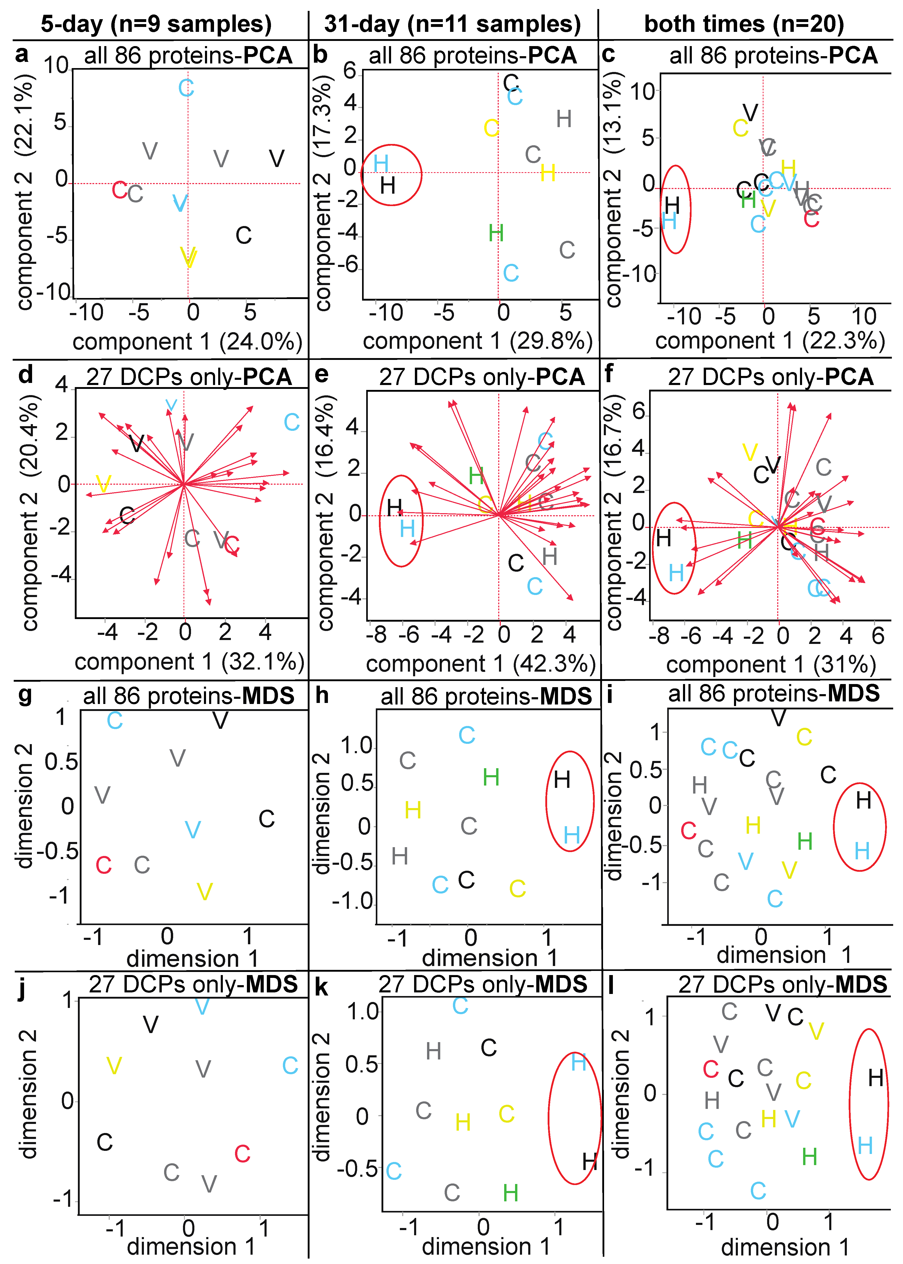
3.3. Proteomic Data Output and Descriptive Multivariate Analyses

A summary of the proteins identified at each quality control step can be found in Table 3. Briefly, 42,316 MS/MS spectra were generated across the three normalizer and 20 experiment coral samples. These spectra were distilled into >37,000 peptides: 17,553 and 19,509 host and endosymbiont proteins, respectively. Of these, ~30% were redundant across samples, leaving approximately 13,000 unique proteins from each compartment. Only 25% of these peptides had iTRAQ tags (~3000/compartment; a common pitfall of label-based proteomics [19]), and an even smaller number (99 host coral and 68 Symbiodiniaceae proteins) were labeled in all three iTRAQ batches. Upon filtering out proteins featuring one only mapped peptide, 46 host coral and 40 Symbiodiniaceae proteins were featured in the analyses discussed below. Although this small subset of proteins was nevertheless capable of resolving certain differences in O. faveolata thermo-sensitivity (discussed below), it is worth noting that other ‘Omics technologies (particularly RNA-Seq-based transcriptome profiling) would surely produce a larger final subset of analytes that could be used in predictive model building.
Temperature effects were not evident in the principal components analysis (Figure 1a,d) or multi-dimensional scaling (Figure 1g,j) biplots of the 5-day samples. As the degree-heating weeks increased from ~1 to 3 (day 31), the two actively bleaching samples (encircled in red in certain panels of Figure 1) clearly demonstrated different proteomes, and this was supported by PERMANOVA of the host coral partial proteome (effect of fragment health designation, p < 0.05; Table 4). In fact, for most, but not all, experimental parameters, the host coral proteome demonstrated greater variation (Table 4); this is in contrast to proteomic analyses of temperature-challenged Indo-Pacific corals [22,23], in which the dinoflagellates demonstrate a more pronounced protein-level response to stress-inducing temperatures. It is worth mentioning, though, that the Indo-Pacific corals analyzed hosted exclusively Cladocopium spp. dinoflagellates, vs. Breviolum and/or Durusdinium in the samples analyzed herein; this could, in part, explain differences in relative proteomic sensitivity to high temperatures among studies.

3.4. Methodological Comparison

A comparison between the results of a “shotgun” proteomic analysis vs. those of the iTRAQ method featured herein can be found in the Supplementary Materials.

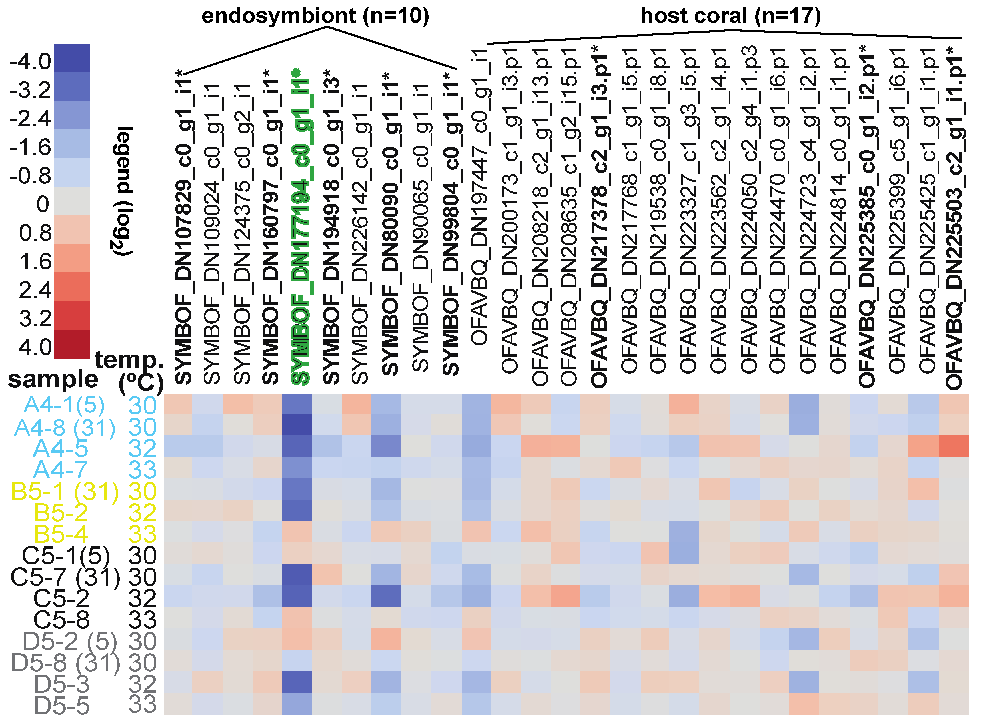
3.5. Differentially Concentrated Proteins

Few proteins were differentially concentrated across the experimental factors; the response screen identified six Symbiodiniaceae and three host coral proteins (Table 5 and Figure 2) that were affected by any of the experimental treatments, and none of these nine were significantly affected by temperature or temperature x time. Instead, reef site and genotype had greater influences on individual protein concentrations, as did fragment health designation (which significantly affected the concentration of one host and one Symbiodiniaceae protein). Of the six unique Symbiodiniaceae differentially concentrated proteins (Table 5), half could not be assigned an identity, and the function of a fourth (apolipoprotein B100 C terminal) could not be inferred bioinformatically (online supplemental data file). The remaining two, tyrosine decarboxylase 1-like and sec34 sodium channel protein 11, are putatively involved in metabolism and protein trafficking, respectively, based on analysis of their conserved domains. The latter was maintained at higher levels in the gastrodermal cells of the corals of Cheeca Rocks relative to offshore corals.
The three coral host differentially concentrated proteins (Table 5)—myosin 11, sacsin (HSP70 co-chaperone), and concanavalin A-like lectin/glucanase—are involved in the musculature, stress response, and cell adhesion, respectively, based on bioinformatic analysis of their conserved domains. The concentration of the former was affected by both shelf and genotype, with inshore genotypes synthesizing higher myosin 11 levels. Sacsin’s concentration was affected only by site; corals of Cheeca Rocks maintained higher levels of this protein. Concanavalin-A was the only host coral protein affected by the fragment health designation, and it was significantly higher in concentration in actively bleaching corals. This well-studied lectin is a mitogen that strongly binds glycoproteins [24], and it has been hypothesized (but never directly shown) to play a role in coral immunity [25]. Although it is tempting to implicate a role of immunity in coral bleaching, it is important to note two things. First, only two samples were actively bleaching at the time of sampling (i.e., low sample size). Secondly, these two samples had already paled markedly at the time of sampling (day-31); as such, this protein is associated with bleaching and not necessarily involved in the bleaching process. Although immunity, as well as host-dinoflagellate interactions, by definition, are inextricably involved in coral bleaching [26], a larger sample size with a more refined temporal sampling scheme would be needed to implicate a role of this lectin in the underlying cellular mechanisms.

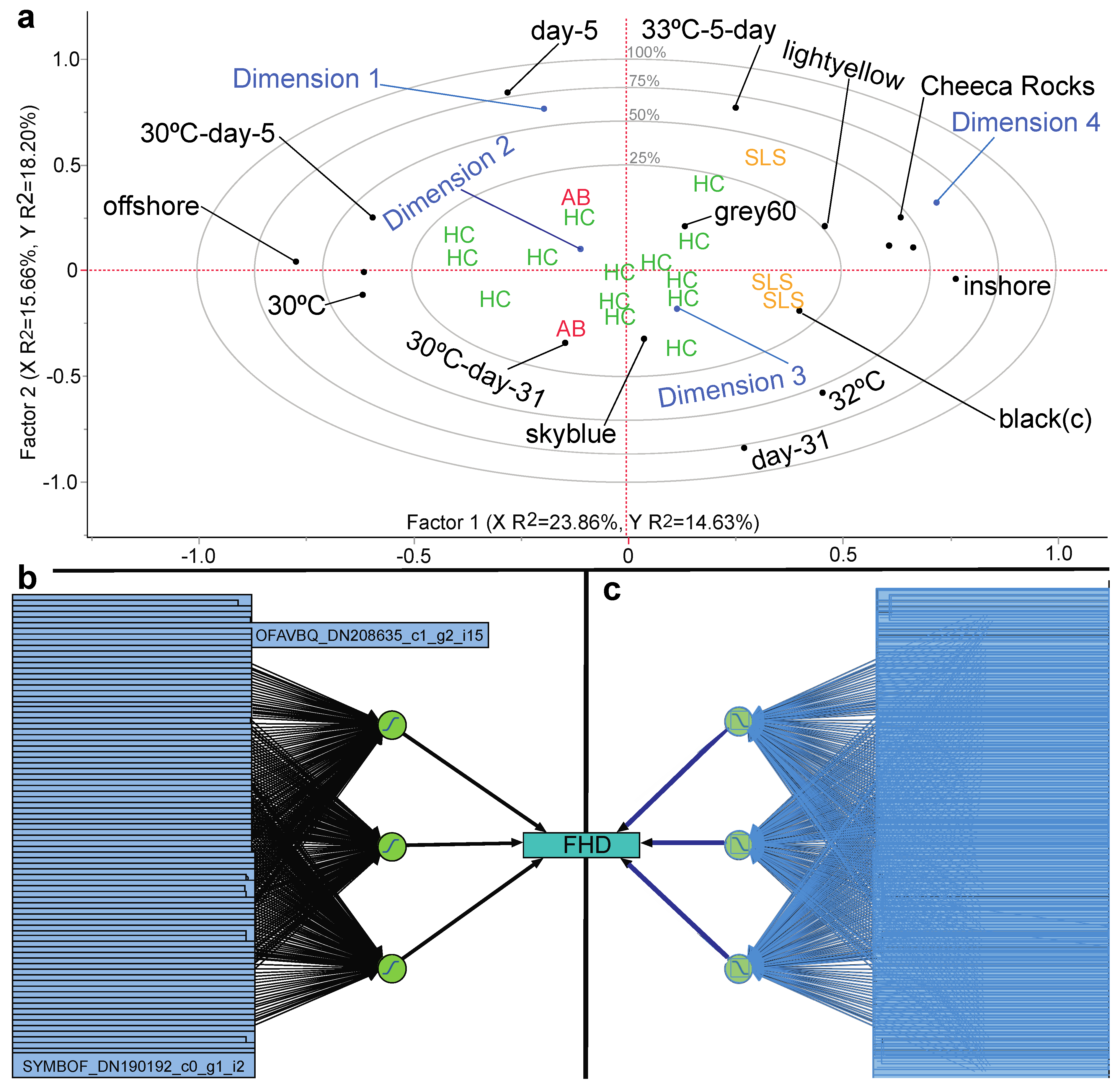
3.6. Stepwise Discriminant Analysis-Based Coral Biomarker Profiling

Although characterized by high training model accuracies for a number of experimental parameters (Figures S1 and S2), the biomarker-based stepwise discriminant analysis validation misclassification rates were high (Table S1); for this reason, these results are discussed in the Supplementary Materials only.

3.7. Proteomic Predictive Modeling of Coral Fragment Condition

A variety of proteomic data-trained predictive models were built in hindcasted manner to attempt to use molecular data to forecast bleaching susceptibility, and, in general, only the machine-learning-based neural networks were capable of accurately predicting the fragment health designation (Table 2, Table 6, Tables S2 and S3). One representative model is shown in Figure 3b,c. The multivariate plots of Figure 1, as well as the partial least squares-based correlation loading plot (Figure 3a) in part highlight why simpler modeling types failed (including the aforementioned stepwise discriminant analysis). From Figure 1, it is clear that the proteomes of the two actively bleaching samples were significantly different from those of the healthy control and sub-lethally stressed corals (corroborated by PERMANOVA; Table 4). As such, a simple modeling type like stepwise discriminant analysis (Figures S1b and S2b) could correctly classify stressed corals (actively bleaching + sub-lethally stressed) from healthy corals at >95% accuracy. However, from Figure 3a, it is clear that there is overlap across the three fragment health designations when looking at all 86 proteins. This explains why, when validating the data in Figures S1b and S2b with holdback samples (or other means), stepwise discriminant analysis model misclassification rates as high as 40% were obtained (Table S1).
Table 5. Differentially concentrated proteins. Site (n = 3: Cheeca Rocks, The Rocks, and Little Conch), shelf (n = 2: inshore vs. offshore), temperature-A (n = 3: 30, 32, and 33 °C), temperature-B (n = 2: control vs. high [pooled over time]), genotype (n = 6; Table 1), time (n = 2: 5 vs. 31 days), temperature x time (n = 4), and fragment health designation (FHD; n = 3) were tested individually in a response screening analysis (false discovery rate-adjusted p < 0.01 with log2-transformed data), and only experimental factors that significantly affected concentrations of at least one protein have been included. When a protein could not be identified, the top BLAST hit against the Symbiodinium microadriaticum genome has been included in parentheses in the “Identity” column. All 11 (9 unique; repeated proteins denoted by *) coral and endosymbiont differentially concentrated proteins featured in the respective stepwise discriminant analysis (i.e., “proteins of interest”) except for SYMBOF_DN177194_c0_g1, which was not included in the endosymbiont stepwise discriminant analysis model of time. Please see Figure S3 for a Venn diagram depicting the degree of differentially concentrated protein vs. protein of interest overlap.
Comparisondf#ProteinsTranscriptome AccessionIdentityTrend
Endosymbionts
TIME121. SYMBOF_DN80090_c0_tyrosine decarboxylase 1-like5 > 31 days
2. SYMBOF_DN177194_c0_g1 bapolipoprotein B100 C terminal5 > 31 days
SITE233. SYMBOF_DN99804_c0_g1 a,bsec34 sodium channel protein 11Cheeca Rocks > Little Conch
4. SYMBOF_DN160797_c0_g1 bunknown (OLQ08781.1)The Rocks + Cheeca Rocks > Little Conch
5. SYMBOF_DN194918_c0_g1 bunknownLittle Conch + Cheeca Rocks > The Rocks
GENOTYPE51 *  SYMBOF_DN160797_c0_g1 bunknown (see also endosymbiont #4.).grey60 > lightyellow
FRAGMENT HEALTH
DESIGNATION
116. SYMBOF_DN107829_c0_g1 bunknown (OLP80463.1)healthy control > actively bleaching
Host coral
SITE211. OFAVBQ_DN225385_c0_g1 c,dsacsinCheeca Rocks > Little Conch + The Rocks
SHELF112. OFAVBQ_DN217378_c2_g1myosin 11-likeinshore > offshore
GENOTYPE51 * OFAVBQ_DN217378_c2_g1myosin 11-like (see also host #2.)grey60 + skyblue > lightyellow
FRAGMENT HEALTH
DESIGNATION
113. OFAVBQ_DN225503_c2_g1concanavalin A-like lectin/glucanaseactively bleaching > healthy control
(1.5-fold)
a protein also affected by shelf: inshore > offshore. b >2-fold difference between most extreme values. c under selection in other coral species [27,28]. d marginal effect of colony health designation: bleaching-resistant > bleaching-susceptible (p < 0.01 [non-false discovery rate-adjusted]).
In contrast, the neural networks (Table 6, Tables S2 and S3) correctly classified the fragment health designation of all validation samples that were held back from the training models, though their drawback is that they require input data from all 86 proteins; were a field coral biopsy analyzed via proteomics, and a different suite of proteins were sequenced (a likely scenario given the stochastic nature of proteomics), a new model would have to be built that would incorporate only those proteins found in all samples. This would surely result in a reduction in the number of proteins in the final model; whether it would also result in diminished accuracy remains to be determined through field-testing of these machine-learning models (discussed below).

3.8. Proteomic Predictive Models of Colony Bleaching Susceptibility

In contrast to the neural network fragment health model, a simpler generalized regression model was capable of accurately forecasting (0% misclassification rate) the colony health designation (Table 2 and Table 6), and, unlike neural networks, generalized regression (i.e., “gen-reg”) permits response variable reduction (both methods accommodate multi-collinearity across response variables.). In the case of the pruned forward selection model (Table 6), only three proteins could accurately forecast whether a colony would be bleaching-susceptible or bleaching-resistant. This predictive power is impressive in that the underlying training samples spanned fragments that were exposed to different treatments and were therefore characterized by different health states (Table 1). In other words, these three proteins represent entrained properties of the original host coral colonies that could be discerned even as the fragments were subjected to elevated temperatures in the laboratory. One of the proteins, SYMBOF_DN194918_c0_g1_i3, was also a differentially concentrated protein, though the function of this Symbiodiniaceae protein could not be deduced from alignment-based bioinformatics approaches. The host coral protein OFAVBQ_DN218976_c2_ g3_i2 also could not be characterized; the top hit (XP_022804074.1; e = 0) was an uncharacterized protein first identified in another coral, Stylophora pistillata.
The final protein in the pruned generalized regression model, OFAVBQ_DN222591_c0_g1_i4, is a 100% match to a published O. faveolata sequence (XP_020618219.1; e = 0) that was annotated as a “polycystic kidney disease and receptor for egg jelly-related protein-like isoform X2.” This is an ion channel hypothetically involved in reproduction [29] or even calcification [30], and, although it missed the false discovery rate-adjusted cutoff for being deemed a differentially concentrated protein (p = 0.02 vs. p < 0.01), it was maintained at 2-fold higher levels in bleaching-resistant vs. bleaching-susceptible corals. It is worth noting that the Symbiodiniaceae homolog, polycystin-2, was also found to be a strong predictor of the colony health designation in the NTanH(3)-NBoost(3) model (Table 6), and it was also up-regulated in the two actively bleaching samples (3-fold over all remaining samples); however, it was not considered a differentially concentrated protein at the false discovery rate-adjusted p-value (p = 0.02). Nevertheless, the fact that the same protein was (1) up-regulated in Symbiodiniaceae within bleaching corals and (2) maintained at higher levels in bleaching-resistant coral hosts signifies that this ion channel not only could be important as a health-informing biomarker, but it could indeed play a role in the cellular mechanism underlying the bleaching process itself; it therefore should be prioritized in future molecular analyses.
It is not always the case that those analytes that best describe a phenomenon are also the best predictors; in fact, this is often not so [31]. However, in this instance, despite not being a differentially concentrated protein, it appears that this ion channel, which has been identified in prior proteomic analyses of corals [32], is a good predictor of colony bleaching susceptibility and demonstrated a marked difference in concentrations between bleaching-resistant and bleaching-susceptible corals in an experimental setting. Of all 86 proteins analyzed, then, this ion channel may be the lone candidate for those looking to measure concentrations of a single biomarker to assess bleaching susceptibility. In contrast, neural network models require measuring all 86 proteins (i.e., no response variable reduction). Whether these models can also predict bleaching susceptibility in field corals remains to be determined but is under active investigation using fate-tracked colonies along the Upper Florida Keys Reef Tract that were sampled before, during, and after a bleaching event in 2019. By inputting the proteomic data from biopsies that did and did not bleach during this bleaching event, I can determine whether the models discussed herein are capable of demarking a colony as bleaching-resistant or bleaching-susceptible before the actual occurrence of visible bleaching (i.e., from the winter-spring, pre-bleaching sampling times, during which the colonies’ health designations would be either healthy or possibly sub-lethally stressed at worse). Based on the partial least squares-based colony health designation correlation loading plot (with dimensionalized data; Figure S5), as well as the high accuracy of the models upon validation with holdback samples (even despite their spanning various fragment health designations), it is likely that such predictive accuracy will be high at the field test sites; in the loading plot, only one bleaching-susceptible sample clustered with the bleaching-resistant samples, and this sample was nevertheless correctly predicted to be bleaching-susceptible based on all colony health designation models listed in Table 6 and Table S3.

3.9. Predicting Coral Colony Resilience with a Molecular Biology + Machine-Learning Approach

Whether or not the bleaching resilience of O. faveolata colonies from locations farther flung from the reefs from which these corals were collected can also be accurately predicted is less certain; massive corals of the Florida Reef Tract have been considerably stress-hardened and/or adapted to highly marginalized conditions over the past decades [17], meaning that a distinctly different model might be needed to discern bleaching-susceptible from bleaching-resistant corals in less impacted locations [33]. Machine-learning approaches are more flexible and can accommodate more complex environmental datasets; although the generalized regression models may maintain utility over the wider Caribbean, the neural network models have theoretically higher potential in this respect. Regardless, field-testing the ability of these complex neural network models to accurately forecast bleaching likelihood (and severity) is the logical next step towards using an ‘Omics + machine-learning approach to model coral health in the Anthropocene. These colony-scale resilience models could then be compared to those trained with exclusively environmental [34,35,36] and/or animal abundance data [37]. With respect to the latter, there is often not a positive association between coral abundance and colony resilience [38]; given this disconnect, a predictive model considering abiotic, ecological, and physiological data will inherently have higher power to forecast timing, intensity, and spatial extent of bleaching than a model featuring only temperature and coral cover (the current most-common predictors). Regardless of the final approach taken, and the predictors incorporated, it will be critical that the models are flexible enough to accommodate phenotypic plasticity and/or organismal adaptation [27,39].

Supplementary Materials

The following are available online at https://www.mdpi.com/article/10.3390/d14010033/s1, Figure S1: Host coral stepwise discriminant analysis. Figure S2: Symbiodiniaceae stepwise discriminant analysis. Figure S3: Venn diagrams depicting relative influence of various environmental predictors on numbers of differentially concentrated proteins (DCPs) and “proteins of interest” (POIs). Figure S4: T2 plot of multivariate variability for the healthy control (HC), sub-lethally stressed (SLS), and actively bleaching (AB) samples. Figure S5: Partial least squares-based correlation loading plot of the 20-sample dataset. Table S1: Additional statistical approaches with log2-transformed protein concentrations. Table S2: Neural networks. Table S3: Additional neural network models whose sample misclassification rates were 0%.

Funding

This work was funded by NOAA (Silver Spring, MD, USA) through the ‘Omics Initiative (NRDD 18978).

Institutional Review Board Statement

A coral collection permit was issued by the Florida Keys National Marine Sanctuary to Derek Manzello (NESDIS, NOAA): #FKNMS-2015-112.

Informed Consent Statement

Not applicable.

Data Availability Statement

In addition to the online supplemental data (Excel) file, the raw and processed proteomic data (as MZML and MZID files) were deposited in two locations: the University of California, San Diego’s (CA, USA) “MassIVE” data repository (accession: MSV000086530) and NOAA’s National Centers for Environmental Information (accession: 0242879).

Acknowledgments

Thanks are given to members of NOAA’s Atlantic Oceanographic and Meteorological Laboratory’s Coral Program for assistance with the tank experiment, and especially Derek Manzello for obtaining the original coral collection permit (referenced above). I am greatly indebted to Diedrich Schmidt (Evonik Superabsorber LLC, Greensboro, NC, USA) for creating the JMP® GUI add-in that allowed for the iterative running of over 20,000 neural networks on a personal laptop with only 8 GB of RAM.

Conflicts of Interest

The author declares no conflict of interest. The funder had no role in the design of the study; in the collection, analyses, or interpretation of data; in the writing of the manuscript, or in the decision to publish the results.

References

  1. Brown, B.E. Coral bleaching: Causes and consequences. Coral Reefs 1997, 16, 129–138. [Google Scholar] [CrossRef]
  2. Grottoli, A.; Toonen, R.J.; van Woesik, R.; Vega-Thurber, R.; Warner, M.E.; McLachlan, R.; Price, J.T.; Bahr, K.D.; Baums, I.B.; Castillo, K.D.; et al. Increasing comparability among coral bleaching experiments. Ecol. Appl. 2021, 31, e02262. [Google Scholar] [CrossRef] [PubMed]
  3. McLachlan, R.H.; Price, J.; Solomon, S.; Grottoli, A.G. Thirty years of coral heat-stress experiments: A review of methods. Coral Reefs 2020, 39, 885–902. [Google Scholar] [CrossRef] [Green Version]
  4. Downs, C.A.; Mueller, E.; Phillips, S.; Fauth, J.E.; Woodley, C.M. A molecular biomarker system for assessing the health of coral (Montastrea faveolata) during heat stress. Mar. Biotechnol. 2020, 2, 533–544. [Google Scholar] [CrossRef] [PubMed]
  5. Parkinson, J.E.; Bartels, E.; Devlin-Durante, M.K.; Lustic, C.; Nedimyer, K.; Schopmeyer, S.; Lirman, D.; LaJeunesse, T.C.; Baums, I.B. Extensive transcriptional variation poses a challenge to thermal stress biomarker development for endangered coral. Mol. Ecol. 2018, 27, 1103–1119. [Google Scholar] [CrossRef]
  6. Mayfield, A.B.; Chen, C.S.; Dempsey, A.C. The molecular ecophysiology of closely related pocilloporid corals of New Caledonia. Platax 2017, 14, 1–45. [Google Scholar]
  7. Mayfield, A.B.; Chen, C.S.; Dempsey, A.C. Biomarker profiling in reef corals of Tonga’s Ha’apai and Vava’u Archipelagos. PLoS ONE 2017, 12, e0185857. [Google Scholar] [CrossRef] [Green Version]
  8. Mayfield, A.B.; Chen, C.S.; Dempsey, A.C. Identifying corals displaying aberrant behavior in Fiji’s Lau Archipelago. PLoS ONE 2017, 12, e0177267. [Google Scholar] [CrossRef] [Green Version]
  9. Mayfield, A.B.; Wang, L.H.; Tang, P.C.; Hsiao, Y.Y.; Fan, T.Y.; Tsai, C.L.; Chen, C.S. Assessing the impacts of experimentally elevated temperature on the biological composition and molecular chaperone gene expression of a reef coral. PLoS ONE 2011, 6, e26529. [Google Scholar] [CrossRef] [Green Version]
  10. Mayfield, A.B.; Aguilar, C.; Enochs, I.; Kolodziej, G.; Manzello, D.P. Shotgun proteomics of thermally challenged Caribbean reef corals. Front. Mar. Sci. 2021, 8, 660153. [Google Scholar] [CrossRef]
  11. Mayfield, A.B.; Wang, Y.B.; Chen, C.S.; Chen, S.H.; Lin, C.Y. Dual-compartmental transcriptomic+proteomic analysis of a marine endosymbiosis exposed to environmental change. Mol. Ecol. 2016, 25, 5944–5958. [Google Scholar] [CrossRef]
  12. Mayfield, A.B.; Chen, Y.J.; Lu, C.Y.; Chen, C.S. Exploring the environmental physiology of the Indo-Pacific reef coral Seriatopora hystrix using differential proteomics. Open. J. Mar. Sci. 2018, 8, 223–252. [Google Scholar] [CrossRef] [Green Version]
  13. Mayfield, A.B.; Chen, Y.J.; Lu, C.Y.; Chen, C.S. The proteomic response of the reef coral Pocillopora acuta to experimentally elevated temperature. PLoS ONE 2018, 13, e0192001. [Google Scholar] [CrossRef] [PubMed] [Green Version]
  14. Aguilar, C.; Enochs, I.; Manzello, D.P.; Mayfield, A.B.; Kolodziej, G.; Carlton, R. Transcriptome profiling of thermotolerant corals of the Upper Florida Keys. Mol. Ecol. unpublished.
  15. Mayfield, A.B.; Chen, C.S. Enabling coral reef triage via molecular biotechnology and artificial intelligence. Platax 2019, 16, 23–47. [Google Scholar]
  16. Manzello, D.P.; Matz, M.V.; Enochs, I.C.; Valentino, L.; Carlton, R.D.; Kolodziej, G.; Serrano, X.; Towle, E.K.; Jankulak, M. Role of host genetics and heat-tolerant algal symbionts in sustaining populations of the endangered coral Orbicella faveolata in the Florida Keys with ocean warming. Glob. Change Biol. 2019, 25, 1016–1031. [Google Scholar] [CrossRef] [Green Version]
  17. Gintert, B.E.; Manzello, D.P.; Enochs, I.C.; Kolodziej, G.; Carlton, R.D.; Gleason, A.C.R.; Gracias, N. Marked annual coral bleaching resilience of an inshore patch reef in the Florida Keys: A nugget of hope, aberrance, or last man standing? Coral Reefs 2018, 37, 533–547. [Google Scholar] [CrossRef] [Green Version]
  18. Siebeck, U.; Marshall, N.; Klüter, A.; Hoegh-Guldberg, O. Monitoring coral bleaching using a colour (sp.) reference card. Coral Reefs 2006, 25, 453–460. [Google Scholar] [CrossRef]
  19. Mayfield, A.B. Proteomic signature of corals from thermodynamic reefs. Microorganisms 2020, 8, 1171. [Google Scholar] [CrossRef]
  20. Desoubeaux, G.; Chauvin, D.; Piqueras, M.C.; Bronson, E.; Bhattacharya, S.K.; Sirpenski, G.; Bailly, E.; Cray, C. Translational proteomic study to address host protein changes during aspergillosis. PLoS ONE 2018, 13, e0200843. [Google Scholar] [CrossRef]
  21. Musada, G.R.; Dvoriantchikova, G.; Myer, C.; Ivanov, D.; Bhattacharya, S.K.; Hackam, A.S. The effect of extrinsic Wnt/β-catenin signaling in Muller glia on retinal ganglion cell neurite growth. Dev. Neurobiol. 2020, 80, 98–110. [Google Scholar] [CrossRef] [PubMed]
  22. Mayfield, A.B.; Wang, Y.B.; Chen, C.S.; Chen, S.H.; Lin, C.Y. Compartment-specific transcriptomics in a reef-building coral exposed to elevated temperatures. Mol. Ecol. 2014, 23, 5816–5830. [Google Scholar] [CrossRef] [PubMed] [Green Version]
  23. McRae, C.; Mayfield, A.B.; Fan, T.Y.; Huang, W.B.; Cote, I. Differing proteomic responses to high-temperature exposure between adult and larval reef corals. Front. Mar. Sci. 2021, 8, 716124. [Google Scholar] [CrossRef]
  24. Reeke, G.N.; Becker, J.W.; Cunningham, B.A.; Wang, J.L.; Yahara, I.; Edelman, G.M. Structure and function of concanavalin A. Adv. Exp. Med. Biol. 1975, 55, 13–33. [Google Scholar] [PubMed]
  25. Vidal-Dupiol, J.; Ladrière, O.; Meistertzheim, A.L.; Fouré, L.; Adjeroud, M.; Mitta, G. Physiological responses of the scleractinian coral Pocillopora damicornis to bacterial stress from Vibrio corallilyticus. J. Exp. Biol. 2011, 214, 1533–1545. [Google Scholar] [CrossRef] [PubMed] [Green Version]
  26. Gates, R.D.; Baghdasarian, G.; Muscatine, L. Temperature stress causes host cell detachment in symbiotic cnidarians: Implications for coral bleaching. Biol. Bull. 1992, 182, 324–332. [Google Scholar] [CrossRef]
  27. Bay, R.A.; Rose, N.H.; Logan, C.A.; Palumbi, S.R. Genomic models predict successful coral adaptation if future ocean warming rates are reduced. Sci. Adv. 2017, 3, e1701413. [Google Scholar] [CrossRef] [PubMed] [Green Version]
  28. Fuller, Z.; Mocellin, V.J.L.; Morris, L.A.; Cantin, N.; Shepherd, J.; Sarre, L.; Peng, J.; Liao, Y.; Pickrell, J.; Andolfatto, P.; et al. Population genetics of the cooral (sp.). Acropora millepora: Toward genomic prediction of bleaching. Science 2020, 369, eaba4674. [Google Scholar]
  29. Cunning, R.; Bay, R.A.; Gillette, P.; Baker, A.C.; Traylor-Knowles, N. Comparative analysis of the Pocillopora damicornis genome highlights role of immune system in coral evolution. Sci. Rep. 2018, 8, 16134. [Google Scholar] [CrossRef] [Green Version]
  30. Parisi, M.G.; Parrinello, D.; Stabili, L.; Cammarata, M. Cnidarian immunity and the repertoire of defense mechanisms in anthozoans. Biology 2020, 9, 283. [Google Scholar] [CrossRef]
  31. Shmueli, G. To explain or to predict? Stat. Sci. 2011, 25, 289–310. [Google Scholar]
  32. Ramos-Silva, P.; Kaandorp, J.; Huisman, L.; Marie, B.; Zanella-Cléon, I.; Guichard, N.; Miller, D.J.; Marin, F. The skeletal proteome of the coral Acropora millepora: The evolution of calcification by co-option and domain shuffling. Mol. Biol. Evol. 2013, 30, 2099–2112. [Google Scholar] [CrossRef] [PubMed]
  33. Roach, T.N.F.; Dilworth, J.; Christian, M.H.; Jones, D.; Quinn, R.A.; Drury, C. Metabolomic signatures of coral bleaching history. Nat. Ecol. Evol. 2021, 5, 495–503. [Google Scholar] [CrossRef]
  34. Maynard, J.A.; Anthony, K.R.N.; Marshall, P.A.; Masiri, I. Major bleaching events can lead to increased thermal tolerance in corals. Mar. Biol. 2008, 155, 173–182. [Google Scholar] [CrossRef]
  35. Liu, G.; Heron, S.F.; Eakin, C.M.; Muller-Karger, F.E.; Vega-Rodriguez, M.; Guild, L.S.; De La Cour, J.L.; Geiger, E.F.; Skirving, W.J.; Burgess, T.F.; et al. Reef-scale thermal stress monitoring of coral ecosystems: New 5-km Global Products from NOAA Coral Reef Watch. Remote Sens. 2014, 6, 11579–11606. [Google Scholar] [CrossRef] [Green Version]
  36. Van Hooidonk, R.; Maynard, J.; Tamelander, J.; Gove, J.; Ahmadia, G.; Raymundo, L.; Williams, G.; Heron, S.F.; Planes, S. Local-scale projections of coral reef futures and implications of the Paris Agreement. Sci. Rep. 2016, 6, 39666. [Google Scholar] [CrossRef]
  37. McClanahan, T.R.; Darling, E.S.; Maina, J.M.; Muthiga, N.A.; D’agata, S.; Jupiter, S.D.; Arthur, R.; Wilson, S.K.; Mangubhai, S.; Nand, Y.; et al. Temperature patterns and mechanisms influencing coral bleaching during the 2016 El Niño. Nat. Clim. Change 2019, 9, 845–851. [Google Scholar] [CrossRef]
  38. Mayfield, A.B.; Bruckner, A.W.; Chen, C.H.; Chen, C.S. A survey of pocilloporids and their endosymbiotic dinoflagellate communities in the Austral and Cook Islands of the South Pacific. Platax 2015, 12, 1–17. [Google Scholar]
  39. Logan, C.A.; Dunne, J.P.; Eakin, C.M.; Donner, S.D. Incorporating adaptive responses into future projections of coral bleaching. Glob. Change Biol. 2014, 20, 125–139. [Google Scholar] [CrossRef]
Figure 1. Multivariate analysis of a partial Orbicella faveolata-Symbiodiniaceae proteome. Principal components analysis (PCA; (af)) was carried out with the 86 proteins that passed all quality control ((ac); biplot rays excluded due to spatial constraints), as well as the 27 differentially concentrated proteins (DCPs; including the “proteins of interest” [POIs]; (df)) for the 5-day ((a,d), respectively), 31-day ((b,e), respectively), and all 20 samples ((c,f), respectively). As a comparison, multi-dimensional scaling (MDS; (gl)) was carried out with all 86 proteins (gi) and the 27 DCPs + POIs (jl). In all panels, the “C,” “H,” and “V” icons represent samples of the control (30 °C), high (32 °C), and very high (33 °C) temperature treatments, respectively, and icons are colored by their 2b-RAD genotype name (e.g., “skyblue” genotype samples colored sky blue) except for genotypes black (b) and black (c), which are colored red and green, respectively. In (b,c,e,f,h,i), red ellipses denote two samples that were actively bleaching at the time of sampling.
Diversity 14 00033 g001
Figure 2. Heat map of differentially concentrated proteins (bold font with asterisks; n = 9 (Table 5)) and stepwise discriminant analysis-derived “proteins of interest” (n = 18) for a subset of 15 of the 20 coral samples (those for which the same genotype was tested across multiple treatments). The lone differentially concentrated protein identified by the response screen that was not also a protein of interest has been highlighted in green (see also Figure S3). Please note that those samples exposed to 32 or 33 °C were sampled after 31 and 5 days, respectively; for control (30 °C)-temperature samples, the sampling time (in days) has been included in parentheses next to the sample code. Also note that the protein isolated from the B5 genotype fragment at the 5-day sampling time was compromised during the protein library preparation and not analyzed.
Diversity 14 00033 g002
Figure 3. Partial least squares correlation loading plot and a representative neural network for forecasting coral bleaching susceptibility. In the three-factor, NIPALS-fit loading plot ((a); first two factors shown only), the black dots represent model terms (environmental predictors, e.g., genotype) that correlated strongly with the dimensionalized data (first four multi-dimensional scaling coordinates; in blue) for the three fragment health designations (FHD): healthy controls (HC), sub-lethally stressed (SLS) samples, and actively bleaching (AB) coral fragments. In the representative, TanH-activated, tri-nodal neural network ((b); kfold validation of five), the squared penalty method was used with a single tour (two “boosted” models with a learning rate of 0.1), and the blue boxes encapsulate the 86 proteins (of which a representative host coral and Symbiodiniaceae protein has been shown). The misclassification rate of this model was 0% (validation root-mean square error = 0.64). To better highlight its structure, a mirror image has been shown (c) in which interior linkages are more clearly seen. See Figure S5 for an analogous colony health designation partial least squares correlation loading plot. In total over 21,000 neural networks were tested and simulated (Table S2 and online supplemental data file).
Diversity 14 00033 g003
Table 1. Details of the experimental iTRAQ samples. Please note that one sample (denoted by *) spilled in the speed-vac during preparation and so was not analyzed. AB = actively bleaching (n = 2), BLR = bleaching-resistant (n = 14), BLS = bleaching-susceptible (n = 6), HC = healthy control (n = 10), HTA = high-temperature-acclimating (n = 5), ID = indeterminant (not enough data to determine; n = 1), and SLS = sub-lethally stressed (n = 3). For the raw proteomic data, please see the “host-batch A–C” and “endosymbiont-batch A–C” worksheets in the online supplemental data file. NA = not applicable.
Sample NameReef of OriginShelfTreatment (Temp. × Time)GenotypeColony CodeHealth DesignationProtein Loaded (µg)iTRAQ TagiTRAQ Batch
ColonyFragment
Normalizermix of allmix of bothmix of allmix of allNANANA22113A
B5-7 *Cheeca Rocksinshore30-5lightyellowB5BLRHC22114A
C5-1Little Conchoffshore30-5black(a)C5BLSHC22115A
B5-4Cheeca Rocksinshore33-5lightyellowB5BLRSLS22116A
A2-2The Rocksinshore30-31skyblueA2BLSHC22117A
A4-5The Rocksinshore32-31skyblueA4BLRHTA22118A
B3-1Cheeca Rocksinshore32-31black(c)B3BLRHTA22119A
C5-2Little Conchoffshore32-31black(a)C5BLSAB22121A
Normalizermix of allmix of bothmix of allmix of allNANANA22113B
A4-1The Rocksinshore30-5skyblueA4BLRHC22114B
C2-2Little Conchoffshore30-5black(b)C2BLSHC22115B
D5-2Cheeca Rocksinshore30-5grey60D5BLRHC22116B
D6-6Cheeca Rocksinshore33-5grey60D6IDSLS22117B
A4-8The Rocksinshore30-31skyblueA4BLRHC22118B
C5-7Little Conchoffshore30-31black(a)C5BLSHC22119B
D5-3Cheeca Rocksinshore32-31grey60D5BLRHTA22121B
Normalizermix of allmix of bothmix of allmix of allNANANA22113C
A4-7The Rocksinshore33-5skyblueA4BLRHTA22114C
C5-8Little Conchoffshore33-5black(a)C5BLSAB22115C
D5-5Cheeca Rocksinshore33-5grey60D5BLRHTA22116C
B5-1Cheeca Rocksinshore30-31lightyellowB5BLRHC22117C
D4-8Cheeca Rocksinshore30-31grey60D4BLRHC22118C
D5-8Cheeca Rocksinshore30-31grey60D5BLRHC22119C
B5-2Cheeca Rocksinshore32-31lightyellowB5BLRSLS22121C
Table 2. Statistical approaches. Only the approaches that yielded statistically significant results, identified differentially concentrated proteins (Table 3), or correctly predicted coral bleaching susceptibility with high accuracy have been shown; please see Table S1 for a complete list of all methods employed. CHD = colony health designation (bleaching-susceptible vs. bleaching-resistant). EP = experimental parameter (e.g., temperature). FDR = false discovery rate. FHD = fragment health designation (the status of the coral fragment at time of sampling). GMR = generalized multivariate regression (also known as “gen-reg”). MDS = multi-dimensional scaling. MPM = model percent misclassified. NA = not applicable. PERMANOVA = permutational multivariate analysis of variance.
Analytical Goal
Approach
Response Variables (Y)/Predictors (X)Acceptance
Criterion (a)
Primary Finding (s)Data Location (s)
Uncover multivariate treatment effects
 PERMANOVA86 proteins/all EPalpha = 0.05Effect of fragment health designation on host proteomeTable 4
 Non-parametric MANOVAMDS coordinates/
all EP
MDS stress < 0.1 and alpha = 0.05Effect of reef site on host and holobiont proteomesTable 4
Identify differentially concentrated proteins
 Response screening analysis86 proteins/all EPFDR-p < 0.019 differentially concentrated proteins identifiedTable 5 and Figure 2
 Stepwise discriminant analysis86 proteins/all EPMPM < 15% a18 “proteins of interest” identifiedTable 5, Figures S1 and S2
Predict bleaching susceptibility
Fragment health designation (FHD; 15/5 training/validation samples)
  Neural networkFHD/86 proteinsMPM < 10%Only model type with high accuracyTable 6, Tables S2 and S3
Colony health designation (CHD; 15/5 training/validation samples)
  Neural networkCHD/86 proteinsMPM < 10%More flexible than GMR modelsTable 6, Tables S2 and S3
  GMR-lassoCHD/86 proteinsMPM < 10%All 86 proteins in final model Table 6
  GMR-pruned forward selectionCHD/86 proteinsMPM < 10%Three proteins in final model Table 6
a Please note that validation MPM values were significantly higher (Table S1).
Table 4. Permutational MANOVA (PERMANOVA). PERMANOVA of a Euclidean distance matrix built from standardized, log2-transformed data using an unrestricted permutation of raw data (sum of squares type III) model. One significant finding (p < 0.05) has been highlighted in bold. NA = not applicable. PERMDISP = test of homogeneity of dispersion (to determine whether multivariate variance across samples within each experimental bin differed significantly from others under the treatment of interest). In general, multivariate variability was only found to differ significantly across genotypes; some genotypes were more variable than others in their multivariate response (Figure S4). When a non-parametric MANOVA (NP-MANOVA) based on coordinates from the first six, seven, and seven dimensions for the endosymbiont (multi-dimensional scaling stress = 0.06), host coral (stress = 0.07), and holobiont datasets (stress = 0.07), respectively, yielded a conflicting finding, the model term has been underlined.
FactordfPseudo Fp#PermutationsMultiple PERMANOVA Comparisons
or NP-MANOVA Differences
Endosymbiont—40 proteins
Temperature (n = 3)20.9250.579998
Temperature (n = 2)10.8120.657990
Site21.330.106998
Shelf11.240.219965
Genotype *51.0370.407999
Day11.170.300994
Temperature × day11.0950.380999
Fragment health designation11.0710.383965
Host coral—46 proteins
Temperature (n = 3)21.270.140998
Temperature (n = 2)11.160.280991
Site a21.330.128998Significant site effect by NP-MANOVA
Shelf11.200.229964
Genotype *51.230.153998Black(a) ≠ grey60 ≠ skyblue ≠ lightyellow
Day11.0270.381993
Temperature × day11.0920.296996
Fragment health designation11.900.025969Sub-lethally stressed = actively bleaching ≠ healthy control
Host + endosymbiont—all 86 proteins
Temperature (n = 3)21.110.289998
Temperature (n = 2)11.0020.432989
Site21.320.100997Significant site effect by NP-MANOVA
Shelf11.180.199958
Genotype *51.0960.271997
Day11.0880.355995
Temperature × day11.0490.364999
Fragment health designation11.470.081971
* PERMDISP p < 0.05. a PERMDISP p = 0.06.
Table 6. Representative neural network and generalized multivariate regression models for predicting coral bleaching susceptibility. Of all optimizable model input parameters for neural networks, only the number of tours significantly affected model performance; more tours resulted in superior models. All neural networks feature a single hidden layer. When three numbers appear in the “Validation” column, they correspond to training, validation, and test samples, respectively. All fragment health designation models featured three categories (i.e., healthy controls and high-temperature-acclimating samples were combined.). Please note that, with the exception of the pruned generalized multivariate regression (gen-reg) model, the “Highly influential protein(s)” represent a subset of all proteins featured in the model. MPM = model percent misclassified (i.e., 1 minus accuracy). NA = not applicable. RMSE = root mean square error. WD = weight decay. * featured in additional models.
Model NameValidation#ProteinsType of Activation (# Nodes)#Boosts (Learning Rate)# ToursPenalty MethodTraining RMSETraining MPM (%)Validation RMSEValidation MPM (%)Highly Influential Protein(s)Protein Identity
Fragment health designation
NTanH(2)-NBoost(2)15/586sigmoidal(2)2 (0.1)100WD0.0200.040SYMBOF_DN160797_c0_g1 a SYMBOF_DN231313_c0_g1_i1 OFAVBQ_DN225382_c1_g1_i3integrin-linked protein kinase serine/arginine-rich splicing factor 2 unknown protein w/ HEAT repeats
NTanH(4)-NLinear(1)-NGaussian(1)-NBoost(2)Kfold(5)86sigmoidal(4) linear(1) radial(1)2 (0.1)100WD<0.000<0.000SYMBOF_DN177194_c0_g1 a SYMBOF_DN156077_c0_g1_i1 SYMBOF_DN102933_c0_g1_i1cilia & flagella-associated protein 57
tRNA (Ile)-lysidine synthase
calcium-dependent protein kinase 2
NTanH(2)-NLinear(4)-NGaussian(4)Kfold(5)86sigmoidal(2) linear(4) radial(4)0100absolute<0.000<0.000OFAVBQ_DN208218_c2_g1_i13 OFAVBQ_DN220422_c1_g2_i1 OFAVBQ_DN225382_c1_g1_i3histone-lysine N-methyltransferase
unknown
unknown protein w/ HEAT repeats *
NTanH(3) bhold-back(0.33)86sigmoidal(3)0100WD0.250.080.050OFAVBQ_DN224050_c2_g4_i1 SYMBOF_DN156997_c0_g1_i1
SYMBOF_DN147436_c0_g1_i2
unknown w/endonuclease domain
reticulocyte-binding protein 2 homolog a
unknown protein w/ PHD finger 1 domain
NTanH(3)-NBoost(5)Kfold(5)86sigmoidal(3)5 (0.1)1squared<0.000<0.000OFAVBQ_DN222591_c0_g1_i4 SYMBOF_DN244033_c0_g1_i1 SYMBOF_DN156077_c0_g1_i1PKD with egg jelly receptor c
DNA helicase ETL1
unknown
Colony health designation
NTanH(3)-NBoost(3)Kfold(5)86sigmoidal(3)3 (0.1)100WD0.290.130.280OFAVBQ_DN217378_c2_g1 a SYMBOF_DN239782_c0_g1_i1 SYMBOF_DN99804_c0_g1 amyosin-11-like (see Table 5)
polycystin-2
sec34 sodium channel protein 11
NLinear(3)13/686linear(3)020squared0.0100.070SYMBOF_DN80090_c0_g1 a SYMBOF_DN177194_c0_g1 a OFAVBQ_DN217378_c2_g1 atyrosine decarboxylase 1-like
apolipoprotein B100 C terminal
myosin-11-like (see Table 5) *
Gen-reg with pruned forward selectionKfold(5)3NANANANA<0.0000.110OFAVBQ_DN218976_c2_g3_i2 OFAVBQ_DN222591_c0_g1_i4 SYMBOF_DN194918_c0_g1_i3 aunknown
PKD with egg jelly receptor c
unknown
Gen-reg-ridge regressionKfold(5)86NANANANA0.0300.400OFAVBQ_DN190522_c0_g2_i1 OFAVBQ_DN197447_c0_g1_i1 OFAVBQ_DN225239_c1_g1_i3unknown
vitellogenin-2
calcineurin-binding protein cabin-1
a Differentially concentrated protein. b Featured in Figure 3b. c polycystic kidney disease and receptor for egg jelly-related protein (closely related to polycystin-2; see SYMBOF_DN239782_c0_g1_i1.).
Publisher’s Note: MDPI stays neutral with regard to jurisdictional claims in published maps and institutional affiliations.

