Perceptions of Similarity Can Mislead Provenancing Strategies—An Example from Five Co-Distributed Acacia Species

Abstract

Ecological restoration requires balancing levels of genetic diversity to achieve present-day establishment as well as long-term sustainability. Assumptions based on distributional, taxonomic or functional generalizations are often made when deciding how to source plant material for restoration. We investigate this assumption and ask whether species-specific data is required to optimize provenancing strategies. We use population genetic and environmental data from five congeneric and largely co-distributed species of Acacia to specifically ask how different species-specific genetic provenancing strategies are based on empirical data and how well a simple, standardized collection strategy would work when applied to the same species. We find substantial variability in terms of patterns of genetic diversity and differentiation across the landscape among these five co-distributed Acacia species. This variation translates into substantial differences in genetic provenancing recommendations among species (ranging from 100% to less than 1% of observed genetic variation across species) that could not have been accurately predicted a priori based on simple observation or overall distributional patterns. Furthermore, when a common provenancing strategy was applied to each species, the recommended collection areas and the evolutionary representativeness of such artificially standardized areas were substantially different (smaller) from those identified based on environmental and genetic data. We recommend the implementation of the increasingly accessible array of evolutionary-based methodologies and information to optimize restoration efforts.

1. Introduction

Ecological restoration is carried out with a multitude of specific goals [1] but in general should always contribute positively to biodiversity, human health and wellbeing and the delivery of ecosystem services [2]. As global interest in restoring ecosystems is growing (e.g., the United Nations’ Decade on Ecosystem Restoration; https://www.decadeonrestoration.org/), it is imperative that targets and actions rely on the best available evidence. The science in support of restoration activities is advancing rapidly [3,4] but to have useful impact, we need to understand what information is generalizable and broadly applicable, and when data is needed. For instance, increasing evidence advocates that promoting genetic diversity will improve the long-term sustainability of restored populations [5,6]. A range of carefully crafted germplasm-sourcing strategies has been proposed to facilitate such practices, but the majority of these (26 at last count [3]) are hampered by the paucity of information needed to identify the genetic and climatic boundaries on which they are based [7]. Therefore, in practice, restoration actions often rely on generalizations about evolutionary boundaries and/or climatic suitability [8]. Yet the evidence and methodological approaches necessary for appraising the suitability of taxonomic, distributional or other types of generalization are scarce at best [9]. We avail of novel standardized datasets and methodological approaches to test if generalized provenancing strategies are reliable.

Evolutionary resilience is critical to restoration success [10], and full recovery is only achieved when all key ecosystem attributes closely resemble those of a reference ecosystem, including the capacity of species and communities to adapt and evolve [2]. The restoration of evolutionarily sustainable ecosystems and biodiversity is therefore reliant on the establishment of a strong link between contemporary fitness and longer-term evolutionary potential [11,12]. As the necessary evolutionary, ecological and environmental information is rarely available, surrogate approaches are often relied upon to provide arbitrary guidance to seed sourcing strategies [13].

Assumptions on the distribution of genetic diversity can potentially be misleading, and while “local is best” [14] is increasingly viewed as a testable experimental hypothesis rather than a universal rule [3], prioritizing areas of high diversity for one species is unlikely to capture the same degree of diversity for another. Provenancing strategies invoking the inclusion of broad genetic representativeness [5,15], climate-adjusted strategies [16] or the use of climatological data [17] generally assume that a replicated approach is applicable across multiple species or, at a minimum, across related and/or co-distributed ones. Generalized expectations on the distribution of genetic diversity can originate from multi-species metanalyses (e.g., [18] using a wide range of sampling and analytical strategies; [19] relying on a more constrained but replicated approach) but it remains challenging to define replicable provenancing strategies from such studies alone.

Here we present a multispecies study aimed at testing the validity of provenancing generalizations based on taxonomic, distributional and functional similarity. We selected five Acacia species with overlapping distributions across the Sydney Basin Bioregion and along the east coast of Australia (Figure 1). The genus Acacia (Mimosaceae) is used extensively for restoration practices in Australia and globally (e.g., http://acaciatreeproject.com.au/acacia-tree-project/). In Australia acacias also have an important role in ecosystem function and dynamics, as they are prolific post-disturbance colonizers recruiting from soil seed banks, contributing to nitrogen fixation and providing food and shelter for a vast array of insects and vertebrates [20].

Comparative investigations involving species representing functional or taxonomic groups commonly used in restoration practices can provide a better understanding of the relative strength of simplified provenancing strategies. This is particularly relevant when extensive overlaps in distribution, ecology and phylogeny are likely to impart localised practitioner communities with an expectation for evolutionary similarities. In order to test the validity of provenancing generalizations, we apply novel standardized methodologies and datasets across five co-distributed acacias frequently used in restoration practices and ask if overlap in distributional patterns mirror: (1) habitat preferences; (2) landscape-genomic patterns; and (3) empirically or arbitrarily defined genetic provenancing boundaries.

2. Materials and Methods

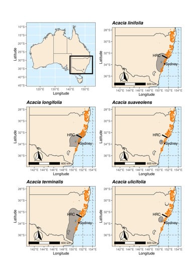
2.1. Study Species: Acacia linifolia, A. longifolia, A. suaveolens, A. terminalis and A. ulicifolia

The five study species were selected because their distributions overlap within the Sydney Basin Bioregion, with Acacia linifolia largely confined to this region and the other four species extending further along the east coast of Australia often in sympatry (Figure 1). All five species are used in restoration practices across eastern Australia and seed can be purchased commercially, generally with little or no indication of seed origin or collecting strategy. Provenancing and seed sourcing guidelines for acacias are mostly “all-purpose” [21,22], despite the genus being highly speciose (>800 species in Australia alone) and occurring across diverse habitats.

The five study species are broadly similar in ecology but vary in some relevant functional traits (Supplementary Table S1). Insect pollination is assumed for most Acacia species [23], but across the study species information was only available for A. longifolia (insect and wind) and A. terminalis (insect and bird [24]). Only a small number of Acacia have been studied in detail for pollination syndrome, and mating systems are considered as predominantly outcrossing [24]. Amongst the study species, A. longifolia and A. terminalis are recorded as self-incompatible, A suaveolens has a mixed mating system which has been discovered using progeny analysis (van der Merwe; pers. comm.) and A. ulicifolia has been recorded as self-compatible [24]. Acacia species can be both fire sensitive and fire responders (resprouting post fire) often relying on soil-stored seedbanks [25]. Seed viability generally increases with short-term soil storage, while dormancy-breaking temperatures and seed predation can vary between individuals and populations [26].

2.2. Species Distributions and Environmental Niche Models—Comparing Niche Overlap and Future Expectations

We used environmental niche models (ENMs) to define and compare habitat preferences among the five study species. For each species, occurrence points were extracted from the Atlas of Living Australia (http://www.ala.org.au) and filtered to remove records without an attached herbarium voucher. We used spThin [27] to randomly remove records so that each occurrence point was at least 2 km apart. The remaining records were used to create occurrence lists for mainland eastern Australia (−39.1, −20.9, 140.5, 154.0).

For the environmental background data, we obtained 19 bioclimatic and seven geomorphological variables at a spatial resolution of 0.01 degrees (1.1 × 1.1 km at the equator) from eMAST [28]. In order to minimize the influence of covariance on our models, we selected sets of variables with a variance inflation factor <12 [29], which was iteratively calculated using the R package usdm [30]. We excluded variables Bio08, Bio09, Bio18 and Bio19 as they show spatial inconsistencies across the study region. This resulted in 32 environmental backgrounds comprised of different combinations of bioclimatic variables along with slope, aspect, topographic position index, and clay percentage.

We modelled habitat suitability for each species with the maximum entropy algorithm implemented by MaxEnt 3.3.3 [31,32]. We used the R package ENMeval [33] to evaluate the AICc score of different ensembles of parameter settings and environmental backgrounds. The parameter settings we varied included three regularization multipliers (0.5, 1.0, 1.5) and each possible combination of three feature classes (Linear, Quadratic, Product). After a trial on a subset of the data, we selected the “checkerboard 1” method to partition the data in all models. We trained all models on environmental backgrounds constrained to a 200 km radius around occurrence points, though projected across the extent of eastern Australia. We took the mean of the top five performing models (lowest AICc score).

To forecast ENMs for the year 2070, we projected contemporary species environment relationships onto general circulation models (GCMs) obtained from the Climate Model Inter-comparison Project 5 (CMIP5) data repository, accessed via the Lawrence Livermore National Laboratory node (https://esgf-node.llnl.gov/projects/esgf-llnl). Since the climate scenarios simulated by different GCMs vary considerably, we used the top four performing GCMs for eastern Australia (ACCESS1-0, GFDL-CM3, MPI-ESM-LR, MPI-ESM-MR), as previously evaluated by [34]. Separate models were constructed for two representative concentration pathways (RCPs) of greenhouse gases assuming a moderate (RCP = 4.5) versus high (RCP = 8.5) emissions scenario. In total, we produced 40 MaxEnt models for each species (5 model settings × 4 GCMs × 2 emissions scenarios).

We calculated the average and standard deviation of the logistic output of the MaxEnt models for the current climate and the two 2070 emissions scenarios. To visualize areas of high predicted habitat suitability in 2070, the mean logistic habitat suitability of the top five performing models minus 2× the standard error was plotted. In addition, we calculated and plotted the change in habitat suitability availability between the current climate and 2070 climate models with the R package Binned Environmental Change Index (BRECI; [35]).

Using the same environmental variables of the top five MaxEnt models, we estimated niche overlap between species across eastern Australia with the R package dynRB [36]. Values are bounded between 0 and 1, with values near 0 indicating a small overlap and near 1 a large overlap [36]. We calculated overlap of n-dimensional hypervolumes for each set of environmental variables, then took an average of the results and plotted directional overlap between species–pairs with a heatmap.

2.3. A New Site Matching Tool

We developed a companion tool to our Restore and Renew webtool decision-support system (https://www.restore-and-renew.org.au; [7], the R&R SiteMatch tool, which allows users to develop an understanding of the distribution of broadly similar environmental conditions at a chosen location, both now and to account for future climate change. A basic form of site matching is provided by the tool, whereby a few selected “key” environmental drivers are used without reference to a selected species—that is, we consider only physical site similarity independently of the response of species. GIS layers are interrogated at a user-selected location to establish values for each of the key factors. Tolerances are then applied to the extracted values providing an indicative envelope of matching environments. The user is then shown a map of the spatial distribution of GIS grid-cells falling within the combined tolerance region for all factors.

Users can select the combination of environmental factors to be used from mean annual temperature (MAT), mean annual precipitation (MAP), temperature seasonality (TS), precipitation seasonality (PS) and aspect and topographic wetness index (TWI). They can also select a combination of future climate change conditions including moderate versus severe impact scenarios, and forward time steps of 2050 or 2070.

2.4. Sampling Strategy and SNP Datasets

We followed the sampling strategy developed for Restore and Renew, a large project that aims to equip restoration practitioners and land managers with a summary of pertinent evolutionary, environmental and ecological information across multiple species [7]. The sampling strategy ensures even representation across the environmental and geographical distribution of each species while maximizing (when possible) between-species overlaps. To achieve maximum informative power while maintaining resource-effectiveness for wild species [7,37,38], the focus is on increasing the number of sites sampled across the distribution of each species targeting six individuals per site (

Table 1. Summary of sampling strategy (site details in Supplementary Table S2) and genomic data used for each Acacia species. N samples (number of samples analysed, samples with greater than 50% loci missing were removed); N sites (sampled); N raw loci (number of loci generated by DArTseq); N loci (number of loci remaining for the analyses after standard filtering process involving the removal of loci with 20% missingness and with minimum reproducibility of 0.96).

Species	N Samples	N Sites	N Raw Loci	N Loci
Acacia linifolia	168	29	43,111	15,274
Acacia longifolia	166	28	36,787	21,509
Acacia suaveolens	166	29	75,908	14,370
Acacia terminalis	256	44	62,423	24,182
Acacia ulicifolia	159	26	135,357	25,421

; Supplementary Table S2).

All samples were genotyped (Table 1) following the method developed by Diversity Arrays Technology Pty Ltd. (DArT) following previously developed protocols [7,39]. Reduced representation sequencing approaches such as DArTseq enable the cost-effective investigation of evolutionary processes at a genomic scale and the fine-scale examination of genetic variation across landscapes [40]. DArTseq is a high throughput, cost-effective restriction-based, reduced representation genome sequencing method that provides genotype data for thousands of single nucleotide polymorphisms (SNPs) across the genome [41,42]. The genome reduction and library construction method of DArTseq principally follows the methods described by [42]. Recent studies using DArTseq have found that they are highly informative for understanding relationships among populations and species in multispecies studies, particularly with closely related lineages [43,44].

2.5. Comparing Landscap Genomics among Five Co-Distributed Acacia Species

The genotype data for each species were analysed using the three-step workflow process (implemented in R) developed as part of the Restore and Renew project [7]. First, SNP loci of poor quality (reproducibility average <0.96, genotypes missing in >20% of samples) and poor-quality samples (samples missing data in a large proportion of loci) were removed, and SNPs were filtered to only include one SNP per locus to prevent the potential influence of linkage. Secondly, a distance-based network analysis [45] was used to identify outlier samples, whether due to taxonomic misidentification or biological processes (such as recent hybridization). After removal of these outlier samples, a dataset was prepared for each species to obtain landscape genetic measures and to derive the statistical models applied in the Restore and Renew webtool to define provenance boundaries. General population genetics measures were also obtained to provide general comparative parameters rather than in-depth interpretations of biology and dynamics (which will be the focus of dedicated studies).

Comparative measures of genetic diversity at population and whole-species levels included: observed heterozygosity (obs_het); expected heterozygosity (exp_het); allelic richness (ar); inbreeding coefficient (Fis) estimated using the R package diveRsity [46]; and number of private alleles (n_pa) within each site were calculated using the private alleles function from Poppr [47]. Additionally, as the preliminary results of A. ulicifolia suggested that some sites included highly similar individuals, we conducted further investigation to determine the presence of clonality (Supplementary Figure S1). Clonality can impact on diversity estimates and individuals identified as clonal were removed from the dataset.

To quantify genetic distance between sample sites, we calculated pairwise Fst values with the Weir and Hill estimator from the R package SNPRelate [48,49]. Correlation between pairwise Fst and linear population distances (isolation-by-distance, IBD) were assessed using a Mantel test [50], implemented with the R package Vegan [51]. Finally, we used sparse non-negative matrix factorization (sNMF) as implemented in the R package LEA [52] to investigate patterns of population structure across the landscape and assign samples to genetic clusters. sNMF was performed with 10 repetitions for each of the K values tested.

2.6. Comparing Provenance Delineation among Five Co-Distributed Acacia Species

Once the preliminary steps were completed, we estimated the models used to generate information for practitioners [7]. Briefly, these are generalized dissimilarity models (GDMs, implemented with R package gdm [53]), describing the level of genetic dissimilarity (differentiation) between sites as a function predictor variable [54,55]. For each species, we first evaluated how well the spatial distance between pairs of sites explained genetic dissimilarity. For species where spatial distance explained a large fraction of observed variation in pairwise genetic dissimilarity, we did not use additional covariates. For species that exhibited discrete stratification into ancestral population groups (or lineages) and this resulted in substantial unexplained variation (“deviance”) in the GDM, we used ancestral population membership coefficients (as inferred using sNMF) as covariates. For A. suaveolens, we observed high levels of differentiation between highland and lowland sites [7], and consequently we used elevation as a covariate in the GDM, because it provided a better fit than spatial distance and ancestral population coefficients. Having estimated a GDM and using it to make predictions for Fst across the landscape in reference to a nominated site, we predicted the genetically local area surrounding that site by choosing a threshold value of differentiation (in this case Fst = 0.2, with the exception of A. suaveolens where we used Fst = 0.3 to be consistent with the steep grade of intra-specific variation [7]). The prediction of the genetically local area for a nominated location can be generated and displayed rapidly. Note that we avoid excessive extrapolation of model predictions by restricting predicted genetically local areas to fall within a buffered hull around the sampled sites (implemented using R packages inla [56], and rgeos [57]). For models that use ancestral population membership coefficients, spatial surfaces for these covariates were generated by using a kriging procedure that is specifically designed for compositional data (implemented in R package compositions [58] and using the compOKriging function).

We compared coverage of observed genetic diversity within geographically defined regions surrounding a test location by fitting convex hulls to the sequenced samples for taxon to the plot on axes PC1 and PC2 of a genotype-derived principal component analysis (PCA). The two geographic regions were: a) the provenance computed using the GDM for the taxon, and b) a 20 km radius around the test location (representing a general-purpose provenance for seed sourcing [13]). The area of each geographically defined convex hull was interpreted as an index of the coverage of observed genetic diversity captured within that geographic space (provenance) and was compared to the convex hull formed using all available samples for a species (i.e., its overall evolutionary potential).

Concave hulls might also be considered as alternatives to convex hulls and could be used to compute a more constrained or conservative estimate of coverage. However, trials of three concave hull methods described in supplementary material (Supplementary Figures S2–S5) suggest that while producing the same rank ordering of coverage estimates, these alternative methods are computationally less efficient than convex hulls and require the setting of one or two arbitrary parameters, therefore reducing the degree of objectivity in their application. We therefore based all further assessment of coverage on convex hull results.

3. Results

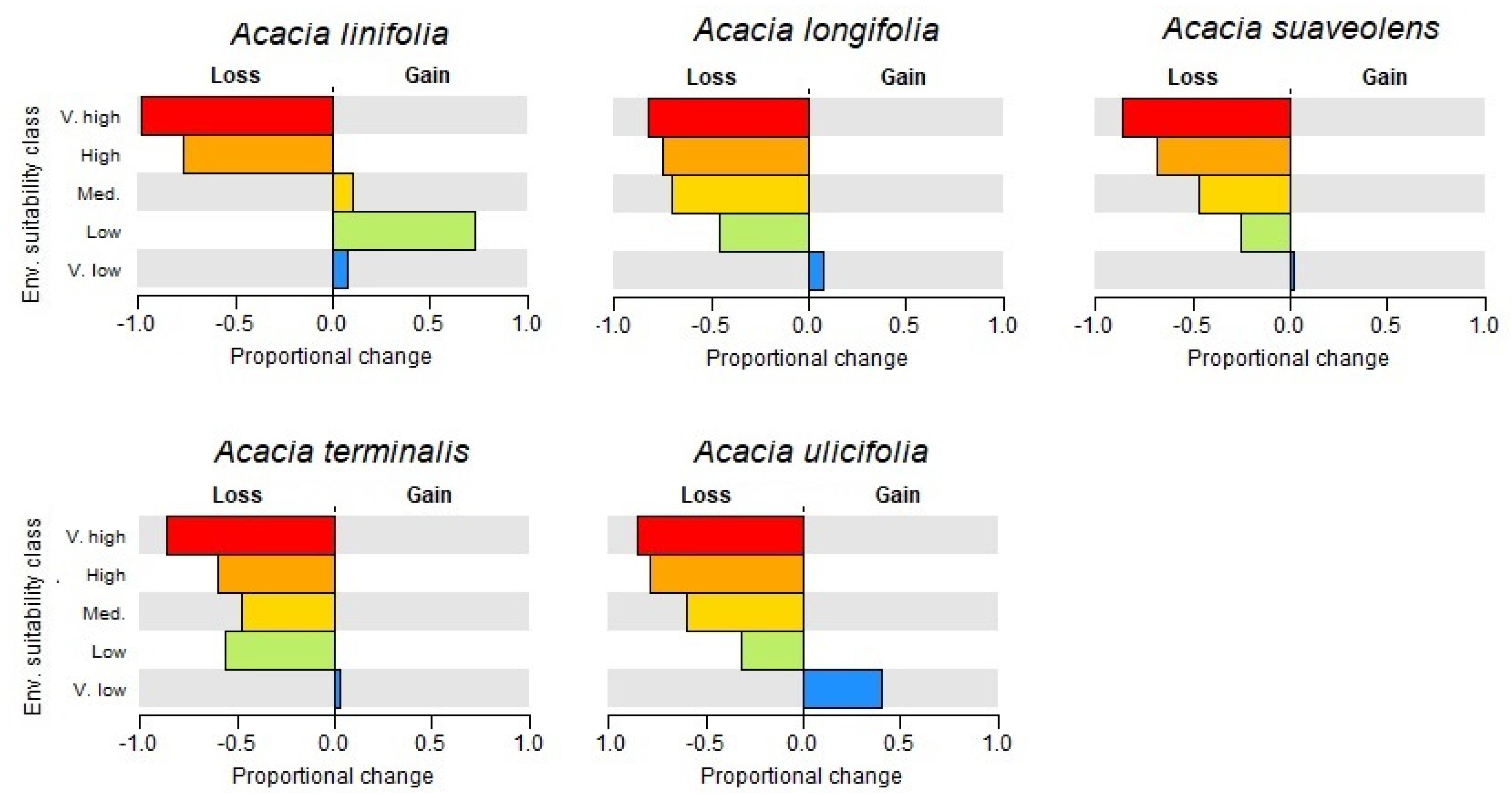
3.1. Species Distributions and Environmental Niche Models—Comparing Niche Overlap and Future Expectations

The comparison of habitat preferences suggests that environmental niche overlap is generally high among the five Acacia species studied (Figure 2). As could be expected, divergence is more evident among species with distribution areas that are particularly different in size, for example between A. linifolia, the species with the smallest distributional range, and all other species. The habitat of A. terminalis also appears to have smaller overlaps in distribution within the northern ranges of the other acacias. Future climate models suggest that the impact of scenarios predicted for 2070 tend to have similar patterns of suitable habitat losses amongst the five acacias, with the species with the smallest distribution being relatively less impacted (Figure 3; Supplementary Figure S6).

Restoration actions which seek to account for local adaptation or “future-proofing” need to characterize the specific environmental condition at a proposed restoration site and to identify regions in the surrounding landscape with broadly similar conditions from which pre-adapted propagation material may be sourced [59]. That is, it is necessary to consider a restricted portion of the species-wide indications of environmental suitability provided by ENMs. Using the site-matching approach, suitable sampling locations that currently characterize future climate conditions can be targeted for climate-proofing restored vegetation across all species (Figure 4). Although less refined than the ENMs, relatively simple site-matching models such as the one developed here provide the opportunity to visualize and interpret overall shifts in local conditions and potential sources of future-adapted material for all the species located at a target site.

3.2. Comparing Knowledge-Based Provenance Delineation and Landscape-Genomics

The genetic provenance boundaries obtained using the predictions from GDMs vary in size and shape among the five species studied (Figure 4). The boundaries defined for Acacia linifolia include the whole range of the species, as expected for a species with little differentiation and a small range. A. longifolia and A. terminalis also displayed large provenance boundaries, although not including the whole species’ distribution and identification of a northern boundary at the Hunter River Corridor, a recognized biogeographic barrier [60]. Finally, A. suaveolens and A. ulicifolia displayed much narrower boundaries, despite the former relying on a higher threshold setting [7].

We used the DArTseq dataset to provide a range of comparative diversity measures at population and whole-species levels for the five study species (Figure 5). The objective here was not to present and interpret a detailed landscape genomics study for each species (to be presented elsewhere), but to provide comparative statistics illustrating the context of this study. Acacia suaveolens displayed lower levels of diversity (allelic and heterozygosity) and higher levels of inbreeding (Fis) than the other species, as well as high levels of between population differentiation (Fst). As previously suggested [7], these high levels of landscape differentiation are reflected in the narrow provenancing boundaries defined for this species. A. ulicifolia showed greater overall variance, and higher levels of observed heterozygosity relative to expected heterozygosity, with higher levels of between-population differentiation (Fst), as expected from a relatively high incidence of population-level clonality (Supplementary Figure S1). Acacia linifolia, A. longifolia and A. terminalis displayed low variance in Fis, while for the other two species levels of inbreeding were more variable across populations. Differences in population dynamics among species are apparent in the relationship between genetic and geographic variation (Figure 6), where varying degrees of isolation by distance (IBD) were identified. Differences in spatial distribution of genetic variation are confirmed by the visualization of genetic structure groups obtained from sNMF analysis (Supplementary Figure S7). A. longifolia, A. suaveolens and A. terminalis appear to have some level of latitudinal structuring, although for each species there are inland populations that are inconsistently grouped with respect to latitude.

Coverage of observed genetic variation captured across the species varied among the five species irrespectively of the methods used to define sourcing boundaries (knowledge based, or arbitrary). The amount of observed genetic variation captured by a 20 km radius region around the test location was found to be a small fraction of coverage provided by provenance regions derived from GDMs (with the exception of A. suaveolens;

Table 2. Coverage of observed genetic variation across the five Acacia species captured by geographic regions defined by using a GDM, and a generic 20 km radius around the same target site. Coverage was computed as the ratio between the area of a convex hull around samples on a plot of PC1 and PC2, and the area of the convex hull around samples falling within the region.

Taxon	Provenance Coverage (Percent)	20 km Radius Coverage (Percent)
Acacia linifolia	100.00	8.18
Acacia longifolia	90.16	5.73
Acacia suaveolens	0.23	0.23
Acacia terminalis	62.72	1.32
Acacia ulicifolia	36.44	0.12

). For example, for Acacia longifolia, a 20 km radius would capture only 5.73% of the total observed genetic variation compared to 90.16% for the GDM-derived provenance and this is clearly seen in the plot of convex hulls for this taxon (Table 2; Supplementary Tables S3 and S4).

4. Discussion

Provenance boundaries empirically estimated from patterns of genetic differentiation were noticeably different among five species of Acacia that are closely tied to an analogous vegetation type and often found in sympatry. We show that broad similarities in habitat requirements among congeneric taxa do not correspond to similar landscape-level dynamics nor to similar distribution of genetic variation. Our data confirms that matching provenancing strategies based on a perception of taxonomic, distributional, environmental or ecological similarities could lead to suboptimal choices. Based on the results presented here, we recommend the implementation of evolutionary-based methodologies to optimize restoration efforts.

Commonalities in the delineation of genetic provenances are unlikely to be the norm, as species respond differently to selective filtering processes and stochastic events through time. The purpose of this study was not to investigate and identify these biological and historical drivers. It is likely however that variations in breeding systems, dispersal mechanisms and response to disturbances gave rise to contrasting patterns of landscape-level connectivity and the genetic provenance boundaries derived from them. For instance, among the five Acacia studied, self-compatibility was only reported for Acacia ulicifolia [24] and A. suaveolens, with current experimentation suggesting that selfing rates and related measures of fitness and viability can vary across a species’ distribution range (van der Merwe pers. comm.).

Differential responses to fire and recruitment from soil seed banks and/or resprouting capacity (Supplementary Table S1) are also likely to impact on the distribution of diversity at population- and species-level. While most Acacia respond to fire through recovery from the seedbank, previous studies suggest that A. ulicifolia and A. terminalis may have mixed responses to post-fire recovery. For example, our genomic data suggest that A. ulicifolia is alone in displaying unexpectedly high levels of clonality (Supplementary Figure S1). Clonality and the potential of resprouting after disturbance events that might have otherwise killed above-ground ramets, can decrease localised vulnerability [61] but can also decrease within-population diversity and increase between-populations divergence (Figure 5). For clonal species, a rapid shift in climate may inflict local extinction due to lack of evolvability and interestingly, A. ulicifolia was the most difficult to collect in consistent numbers with historical occurrence records suggesting localised extinction patterns. Agamospermy could also explain the extensive geographic distribution of clones observed in this study, and while seed production through self-fertilization and agamospermy can both have short term evolutionary benefits (such as range expansion), the levels of genetic diversity captured through seed sourcing will greatly vary depending on the collecting strategy. Consequently, undetected clonality can significantly influence restoration outcomes.

The lack of similarity in provenancing boundaries and the difficulty in developing generalized guidelines [9] is particularly important within highly localized contexts, where practitioners might rely on personal interpretations derived from locally replicated conditions and assemblages (Figure 1 and Figure 2). It has been previously suggested that as anthropogenic influences continue to have an impact on natural systems, the simple protection of standing biodiversity is unlikely to suffice [2,62]. Consequently, restoring vegetation needs to strike a balance between considering natural historical boundaries (as revealed by genetic structure), responding to contemporary conditions (resulting in loss of available habitat for example) and predicting climatic shifts (“future-proofing”). Consequently, the implementation of sourcing strategies that are conscious of both climatic requirements (current or future) and the distribution of genetic diversity, are critical to the success of ecological restoration.

Better access to relevant genomic and environmental data ushered a new era for evolutionarily informed restoration activities [63] and enabled the implementation of novel methodologies that have become cost effective and easy to apply and interpret. Our replicable analytical and interpretational approach suggests that genetic provenancing areas, as defined by natural levels of gene flow, are often large and genetically diverse (Figure 4). The species A. suaveolens was a notable exception. This was possibly due to high levels of selfing or biparental inbreeding in this species (M. van Der Merwe in prep.), leading to high levels of drift and population genetic differentiation, including over relatively short distances. The relatively simple site-matching model developed here provides an additional mechanism to consider climate-related options within these comprehensive, genetically defined sourcing areas (Table 2, Figure 4). Simplifying the logistic requirements of germplasm-sourcing strategies while preventing localized over-harvesting, circumvents some of the limitations of current restoration practices [64].

Finally, while we show that generalized provenancing guidelines and approaches need to be considered with caution, informative replicated patterns are still likely to emerge from large-scale, standardized, multispecies datasets. However, these will not necessarily be based on simple phylogenetic relationships or distributional similarities but will more likely denote shared functional and evolutionary histories [38].

References

1. Clewell, A.F.; Aronson, J. Motivations for the restoration of ecosystems. Conserv. Biol. 2006, 20, 420–428. [Google Scholar] [CrossRef] [PubMed]
2. Gann, G.D.; McDonald, T.; Walder, B.; Aronson, J.; Nelson, C.R.; Jonson, J.; Hua, F. International principles and standards for the practice of ecological restoration. Restor. Ecol. 2019, 27, S1–S46. [Google Scholar] [CrossRef] [Green Version]
3. Jones, T.A. Ecosystem restoration: Recent advances in theory and practice. Rangel. J. 2018, 39, 417–430. [Google Scholar] [CrossRef] [Green Version]
4. Breed, M.F.; Harrison, P.A.; Blyth, C.; Byrne, M.; Gaget, V.; Gellie, N.J.; Steane, D.A. The potential of genomics for restoring ecosystems and biodiversity. Nat. Rev. Genet. 2019, 20, 615–628. [Google Scholar] [CrossRef]
5. Broadhurst, L.M.; Lowe, A.; Coates, D.J.; Cunningham, S.A.; McDonald, M.; Vesk, P.A.; Yates, C. Seed supply for broadscale restoration: Maximizing evolutionary potential. Evol. Appl. 2008, 1, 587–597. [Google Scholar] [CrossRef]
6. St. Clair, A.B.; Dunwiddie, P.W.; Fant, J.B.; Kaye, T.N.; Kramer, A.T. Mixing source populations increases genetic diversity of restored rare plant populations. Restor. Ecol. 2020, 28, 583–593. [Google Scholar] [CrossRef]
7. Rossetto, M.; Bragg, J.; Kilian, A.; McPherson, H.; van der Merwe, M.; Wilson, P.D. Restore and Renew: A genomics-era framework for species provenance delimitation. Restor. Ecol. 2019, 27, 538–548. [Google Scholar] [CrossRef] [Green Version]
8. Hancock, N.; Hughes, L. How far is it to your local? A survey on local provenance use in New South Wales. Ecol. Manag. Restor. 2012, 13, 259–266. [Google Scholar] [CrossRef]
9. Hoban, S.; Callicrate, T.; Clark, J.; Deans, S.; Dosmann, M.; Fant, J.; Gailing, O.; Havens, K.; Hipp, A.L.; Kadav, P.; et al. Taxonomic similarity does not predict necessary sample size for ex situ conservation: A comparison among five genera. Proc. R. Soc. B 2020, 287, 20200102. [Google Scholar] [CrossRef]
10. Kettenring, K.M.; Mercer, K.L.; Reinhardt Adams, C.; Hines, J. Application of genetic diversity–ecosystem function research to ecological restoration. J. Appl. Ecol. 2014, 51, 339–348. [Google Scholar] [CrossRef]
11. Lesica, P.; Allendorf, F.W. Ecological genetics and the restoration of plant communities: Mix or match? Restor. Ecol. 1999, 7, 42–50. [Google Scholar] [CrossRef]
12. Stockwell, C.A.; Kinnison, M.T.; Hendry, A.P.; Hamilton, J.A. Evolutionary restoration ecology. In Foundations of Restoration Ecology; Island Press: Washington, DC, USA, 2016; pp. 427–454. [Google Scholar]
13. Hancock, N.; Gibson-Roy, P.; Driver, M.; Broadhurst, L. The Australian Native Seed Sector Survey Report; Australian Network for Plant Conservation: Canberra, Australia, 2020; Available online: https://www.anpc.asn.au/wp-content/uploads/2020/03/ANPC_NativeSeedSurveyReport_WEB.pdf (accessed on 1 February 2020).
14. McKay, J.K.; Christian, C.E.; Harrison, S.; Rice, K.J. “How local is local?”—A review of practical and conceptual issues in the genetics of restoration. Restor. Ecol. 2005, 13, 432–440. [Google Scholar] [CrossRef]
15. Breed, M.F.; Stead, M.G.; Ottewell, K.M.; Gardner, M.G.; Lowe, A.J. Which provenance and where? Seed sourcing strategies for revegetation in a changing environment. Conserv. Genet. 2013, 14, 1–10. [Google Scholar] [CrossRef]
16. Prober, S.M.; Byrne, M.; McLean, E.H.; Steane, D.A.; Potts, B.M.; Vaillancourt, R.E.; Stock, W.D. Climate-adjusted provenancing: A strategy for climate-resilient ecological restoration. Front. Ecol. Evol. 2015, 3, 65. [Google Scholar] [CrossRef] [Green Version]
17. Massatti, R.; Shriver, R.K.; Winkler, D.E.; Richardson, B.A.; Bradford, J.B. Assessment of population genetics and climatic variability can refine climate-informed seed transfer guidelines. Restor. Ecol. 2020, 28, 485–493. [Google Scholar] [CrossRef]
18. Broadhurst, L.; Breed, M.; Lowe, A.; Bragg, J.; Catullo, R.; Coates, D.; Potts, B. Genetic diversity and structure of the Australian flora. Divers. Distrib. 2017, 23, 41–52. [Google Scholar] [CrossRef] [Green Version]
19. Thiel-Egenter, C.; Gugerli, F.; Alvarez, N.; Brodbeck, S.; Cieślak, E.; Colli, L.; Negrini, R. Effects of species traits on the genetic diversity of high-mountain plants: A multi-species study across the Alps and the Carpathians. Glob. Ecol. Biogeogr. 2009, 18, 78–87. [Google Scholar] [CrossRef]
20. Broadhurst, L.M.; Young, A.G.; Forrester, R. Genetic and demographic responses of fragmented Acacia dealbata (Mimosaceae) populations in southeastern Australia. Biol. Conserv. 2008, 141, 2843–2856. [Google Scholar] [CrossRef]
21. FloraBank. Guidelines 5 Seed Collection from Woody Plants for Local Revegetation; FloraBank: Canberra, Australia, 1999; Available online: http://www.florabank.org.au/ (accessed on 1 February 2020).
22. Gunn, B. Australian Tree Seed Centre Operations Manua; CSIRO Forestry and Forest Products: Canberra, Australia, 2001. [Google Scholar]
23. Bernhardt, P. The floral ecology of Australian Acacia. Adv. Legum. Boil. Monogr. Syst. Bot. Mo. Bot. Gard. 1989, 29, 263–282. [Google Scholar]
24. Kenrick, J.; Knox, R.B. Quantitative Analysis of Self-Incompatibility in Trees of Seven Species of Acacia. J. Hered. 1989, 80, 240–245. [Google Scholar] [CrossRef]
25. Auld, T.D.; O’Connell, M.A. Predicting patterns of post-fire germination in 35 eastern Australian Fabaceae. Aust. J. Ecol. 1991, 16, 53–70. [Google Scholar] [CrossRef]
26. Liyanage, G.S.; Ooi, M.K.J. Intra-population level variation in thresholds for physical dormancy-breaking temperature. Ann. Bot. 2015, 116, 123–131. [Google Scholar] [CrossRef] [PubMed] [Green Version]
27. Aiello-Lammens, M.; Boria, R.; Radosavljevic, A.; Vilela, B.; Anderson, R. spThin: An R package for spatial thinning of species occurrence records for use in ecological niche models. Ecography 2015, 38, 541–545. [Google Scholar] [CrossRef]
28. Xu, T.; Hutchinson, M.F. New developments and applications in the ANUCLIM spatial climatic and bioclimatic modelling package. Environ. Model. Softw. 2013, 40, 267–279. [Google Scholar] [CrossRef]
29. Powney, G.D.; Roy, D.B.; Chapman, D.; Brereton, T.; Oliver, T.H. Measuring functional connectivity using long-term monitoring data. Methods Ecol. Evol. 2011, 2, 527–533. [Google Scholar] [CrossRef] [Green Version]
30. Naimi, B. usdm: Uncertainty analysis for species distribution models. R Package Version 2013, 1, 1–12. [Google Scholar]
31. Phillips, S.J.; Anderson, R.P.; Schapire, R.E. Maximum entropy modeling of species geographic distributions. Ecol. Model. 2006, 190, 231–259. [Google Scholar] [CrossRef] [Green Version]
32. Phillips, S.J.; Dudík, M. Modeling of species distributions with Maxent: New extensions and a comprehensive evaluation. Ecography 2008, 31, 161–175. [Google Scholar] [CrossRef]
33. Muscarella, R.; Galante, P.J.; Soley-Guardia, M.; Boria, R.A.; Kass, J.M.; Uriarte, M.; Anderson, R.P. ENM eval: An R package for conducting spatially independent evaluations and estimating optimal model complexity for Maxent ecological niche models. Methods Ecol. Evol. 2014, 5, 1198–1205. [Google Scholar] [CrossRef]
34. Whetton, P.; Ekström, M.; Gerbing, C.; Grose, M.; Bhend, J.; Webb, L.; Colman, R. Climate Change in Australia. Information for Australia’s Natural Resource Management Regions: Technical Report; 2015. Available online: http://ccia2007.climatechangeinaustralia.gov.au/technical_report.php (accessed on 1 February 2020).
35. Wilson, P.D. Binned Relative Environmental Change Indicator (BRECI): A tool to communicate the nature of differences between environmental niche model outputs. bioRxiv 2019, 672618. [Google Scholar] [CrossRef] [Green Version]
36. Junker, R.R.; Kuppler, J.; Bathke, A.C.; Schreyer, M.L.; Trutschnig, W. Dynamic range boxes—A robust nonparametric approach to quantify size and overlap of n-dimensional hypervolumes. Methods Ecol. Evol. 2016, 7, 1503–1513. [Google Scholar] [CrossRef]
37. Prunier, J.G.; Kaufmann, B.; Fenet, S.; Picard, D.; Pompanon, F.; Joly, P.; Lena, J.P. Optimizing the trade-off between spatial and genetic sampling efforts in patchy populations: Towards a better assessment of functional connectivity using an individual-based sampling scheme. Mol. Ecol. 2013, 22, 5516–5530. [Google Scholar] [CrossRef] [PubMed]
38. Santos, A.S.; Gaiotto, F.A. Knowledge status and sampling strategies to maximize cost-benefit ratio of studies in landscape genomics of wild plants. Sci. Rep. 2020, 10, 3706. [Google Scholar] [CrossRef] [PubMed] [Green Version]
39. Bragg, J.G.; Cuneo, P.; Sherieff, A.; Rossetto, M. Optimizing the genetic composition of a translocation population: Incorporating constraints and conflicting objectives. Mol. Ecol. Resour. 2020, 20, 54–65. [Google Scholar] [CrossRef]
40. Bragg, J.G.; Supple, M.A.; Andrew, R.L.; Borevitz, J.O. Genomic variation across landscapes: Insights and applications. New Phytol. 2015, 207, 953–967. [Google Scholar] [CrossRef] [PubMed]
41. Sansaloni, C.; Petroli, C.; Jaccoud, D.; Carling, J.; Detering, F.; Grattapaglia, D.; Kilian, A. Diversity Arrays Technology (DArT) and next-generation sequencing combined: Genome-wide, high throughput, highly informative genotyping for molecular breeding of Eucalyptus. In BMC Proceedings; BioMed Central: London, UK, 2011; Volume 5, p. 54. [Google Scholar]
42. Kilian, A.; Wenzl, P.; Huttner, E.; Carling, J.; Xia, L.; Blois, H.; Aschenbrenner-Kilian, M. Diversity arrays technology: A generic genome profiling technology on open platforms. In Data Production and Analysis in Population Genomics; Humana Press: Totowa, NJ, USA, 2012; pp. 67–89. [Google Scholar]
43. Rutherford, S.; Rossetto, M.; Bragg, J.G.; McPherson, H.; Benson, D.; Bonser, S.P.; Wilson, P.G. Speciation in the presence of gene flow: Population genomics of closely related and diverging Eucalyptus species. Heredity 2018, 121, 126–141. [Google Scholar] [CrossRef] [PubMed]
44. Fahey, M.; Rossetto, M.; Wilson, P.D.; Ho, S.Y. Habitat preference differentiates the Holocene range dynamics but not barrier effects on two sympatric, congeneric trees (Tristaniopsis, Myrtaceae). Heredity 2019, 123, 532–548. [Google Scholar] [CrossRef]
45. Huson, D.H.; Bryant, D. Application of phylogenetic networks in evolutionary studies. Mol. Biol. Evol. 2006, 23, 254–267. [Google Scholar] [CrossRef]
46. Keenan, K.; McGinnity, P.; Cross, T.F.; Crozier, W.W.; Prodöhl, P.A. diveRsity: An R package for the estimation and exploration of population genetics parameters and their associated errors. Methods Ecol. Evol. 2013, 4, 782–788. [Google Scholar] [CrossRef] [Green Version]
47. Kamvar, Z.N.; Tabima, J.F.; Grünwald, N.J. Poppr: An R package for genetic analysis of populations with clonal, partially clonal, and/or sexual reproduction. PeerJ 2014, 2, e281. [Google Scholar] [CrossRef] [Green Version]
48. Weir, B.S.; Hill, W.G. Estimating F-statistics. Annu. Rev. Genet. 2002, 36, 721–750. [Google Scholar] [CrossRef] [PubMed] [Green Version]
49. Zheng, X.; Zheng, M.X. Package ‘SNPRelate’. A package for Parallel Computing Toolset for Relatedness and Principal Component Analysis of SNP Data. 2013. Available online: http://github.com/zhengxwen/SNPRelate (accessed on 1 February 2020).
50. Mantel, N. The detection of disease clustering and a generalized regression approach. Cancer Res. 1967, 27, 209–220. [Google Scholar] [PubMed]
51. Oksanen, J.; Blanchet, F.G.; Kindt, R.; Legendre, P.; Minchin, P.R.; O’hara, R.B.; Oksanen, M.J. Package ‘vegan’. Community Ecol. Package Version 2013, 2, 1–295. [Google Scholar]
52. Frichot, E.; François, O. LEA: An R package for landscape and ecological association studies. Methods Ecol. Evol. 2015, 6, 925–929. [Google Scholar] [CrossRef]
53. Manion, G.; Lisk, M.; Ferrier, S.; Lugilde, K.M.; Fitzpatrick, M.C.; Fitzpatrick, M.M.C.; Rcpp, I. Package ‘gdm’. A Toolkit with Functions to Fit, Plot, and Summarize Generalized Dissimilarity Models: CRAN Repository, R. 2017. Available online: https://CRAN.R-project.org/package=gdm (accessed on 1 February 2020).
54. Shryock, D.F.; Havrilla, C.A.; DeFalco, L.A.; Esque, T.C.; Custer, N.A.; Wood, T.E. Landscape genetic approaches to guide native plant restoration in the Mojave Desert. Ecol. Appl. 2017, 27, 429–445. [Google Scholar] [CrossRef]
55. Supple, M.A.; Bragg, J.G.; Broadhurst, L.M.; Nicotra, A.B.; Byrne, M.; Andrew, R.L.; Borevitz, J.O. Landscape genomic prediction for restoration of a Eucalyptus foundation species under climate change. eLIFE 2018, 7, e31835. [Google Scholar] [CrossRef]
56. Rue, H.; Martino, S.; Chopin, N. Approximate Bayesian inference for latent Gaussian models using inte-grated nested Laplace approximations (with discussion). J. R. Stat. Soc. Ser. B 2009, 71, 319–392. [Google Scholar] [CrossRef]
57. Bivand, R.; Rundel, C. RGEOS: Interface to Geometry Engine—Open Source (‘GEOS’). R Package Version 0.5-2. 2019. Available online: https://CRAN.R-project.org/package=rgeos (accessed on 1 February 2020).
58. van den Boogaart, K.G.; Tolosana, R.; Bren, M. Compositions: Compositional Data Analysis. R Package Version 1.40-1. 2014. Available online: https://CRAN.R-project.org/package=compositions (accessed on 1 February 2020).
59. Booth, T.H. Identifying particular areas for potential seed collections for restoration plantings under climate change. Ecol. Manag. Restor. 2016, 17, 228–234. [Google Scholar] [CrossRef]
60. Milner, M.L.; Rossetto, M.; Crisp, M.D.; Weston, P.H. The impact of multiple biogeographic barriers and hybridization on species-level differentiation. Am. J. Bot. 2012, 99, 2045–2057. [Google Scholar] [CrossRef]
61. Bond, W.J.; Midgley, J.J. Ecology of sprouting in woody plants: The persistence niche. Trends Ecol. Evol. 2001, 16, 45–51. [Google Scholar] [CrossRef]
62. Parmesan, C. Ecological and evolutionary responses to recent climate change. Annu. Rev. Ecol. Evol. Syst. 2006, 37, 637–669. [Google Scholar] [CrossRef] [Green Version]
63. Williams, A.V.; Nevill, P.G.; Krauss, S.L. Next generation restoration genetics: Applications and opportunities. Trends Plant Sci. 2014, 19, 529–537. [Google Scholar] [CrossRef] [PubMed]
64. Broadhurst, L.; Waters, C.; Coates, D. Native seed for restoration: A discussion of key issues using examples from the flora of southern Australia. Rangel. J. 2018, 39, 487–498. [Google Scholar] [CrossRef]
Figure 1. Distribution of the five study species across the study area of eastern Australia.
Diversity 12 00306 g001
Figure 2. Environmental niche overlap between the five species of Acacia studied across eastern Australia. Overlap is directional, with values reflecting the size of the overlap of the species on the y-axis captured by the niche of the species on the x-axis. Overlap is scored between 0 and 1, with values near 0 indicating a small overlap and near 1 a large overlap. Results presented are the mean across n-dimensional hypervolumes calculated from five different sets of environmental variables and have a minimum overlap of 0.64.
Diversity 12 00306 g002
Figure 3. The proportional change (relative to baseline raster bin values) in habitat suitability between current day and 2070 models calculated in MaxEnt for the five Acacia study species.
Diversity 12 00306 g003
Figure 4. Empirically defined provenance boundaries generated using generalized dissimilarity models (GDMs) based on distribution-wide genomic datasets. All GDMs were evaluated at a common test location (blue teardrop; 33.65° S 150.5° E). GDM-derived provenance is shaded grey. Shaded orange are regions with climate that currently matches predicted 2070 climate at the test location. Matching future climate was assessed under a moderate change scenario (RCP4.5). The location of a major biogeographic barrier, the Hunter River Corridor (HRC), is also included.
Diversity 12 00306 g004
Figure 5. Boxplots of genetic diversity indices for the five Acacia tested. Allelic richness (ar), number of private alleles (n_pa), observed and expected heterozygosity, inbreeding coefficient (Fis) and between population divergence (Fst) are displayed.
Diversity 12 00306 g005
Figure 6. Isolation by distance plots based on pairwise genetic distance (linearized Fst) and geographic distances (log10 transformed) between populations for the five study species.
Diversity 12 00306 g006