Article

Current and Future Distribution of Five Timber Forest Species in Amazonas, Northeast Peru: Contributions towards a Restoration Strategy

by
Nilton B. Rojas Briceño
1,*,
Dany A. Cotrina Sánchez
1,
Elgar Barboza Castillo
1,
Miguel Ángel Barrena Gurbillón
1,
Fausto O. Sarmiento
2,
Diego A. Sotomayor
3,
Manuel Oliva
1 and
Rolando Salas López
1
1
Instituto de Investigación para el Desarrollo Sustentable de Ceja de Selva, Universidad Nacional Toribio Rodríguez de Mendoza de Amazonas, Chachapoyas 01001, Peru
2
Neotropical Montology Collaboratory, Department of Geography, University of Georgia, Athens, GA 30602, USA
3
Departamento de Ingeniería Ambiental, Universidad Nacional Agraria La Molina, La Molina 15012, Peru
*
Author to whom correspondence should be addressed.
Diversity 2020, 12(8), 305; https://doi.org/10.3390/d12080305
Submission received: 18 June 2020 / Revised: 21 July 2020 / Accepted: 22 July 2020 / Published: 8 August 2020

Abstract

:
Forest and land degradation is a serious problem worldwide and the Peruvian National Map of Degraded Areas indicates that 13.78% (177,592.82 km2) of the country’s territory is degraded. Forest plantations can be a restoration strategy, while conserving economically important species affected by climate change and providing forestry material for markets. This study modelled the species distribution under current conditions and climate change scenarios of five Timber Forest Species (TFS) in the Amazonas Department, northeastern Peru. Modelling was conducted with Maximum Entropy (MaxEnt) using 26 environmental variables. Of the total distribution under current conditions of Cedrelinga cateniformis, Ceiba pentandra, Apuleia leiocarpa, Cariniana decandra and Cedrela montana, 34.64% (2985.51 km2), 37.96% (2155.86 km2), 35.34% (2132.57 km2), 33.30% (1848.51 km2), and 35.81% (6125.44 km2), respectively, correspond to degraded areas and, therefore, there is restoration potential with these species. By 2050 and 2070, all TFS are projected to change their distribution compared to their current ranges, regardless of whether it will be an expansion and/or a contraction. Consequently, this methodology is intended to guide the economic and ecological success of forest plantations in reducing areas degraded by deforestation or similar activities.

1. Introduction

Forest and land degradation is a serious problem worldwide, particularly in developing countries [1]. Peru comprises part of the Amazon basin; with approximately 57.4% (739,730 km2) of the territory with forest cover, it is the second largest Amazonian holder in South America and ranks in the top ten countries with the largest global forest area [2]. However, the Peruvian Amazon has lost 22,848.67 km2 of forest between 2001 and 2018, the three of 15 Amazonian departments most affected in the country are San Martin (4365.10 km2), Loreto (4302.80 km2) and Ucayali (3844.70 km2) [3]. The Amazonas Department ranks number eight with 882.79 km2 of lost forest. More than half of this deforestation (ca. 61.8%) is attributed to the expansion of both small-scale farmland (41.9%) and grazing land (19.9%) [4]. Only 1.7% is attributed forest loss due to the establishment of forest plantations. Therefore, Peru’s timber production comes mainly from natural forests [5], where falling is highly selective and is one of the causes of small-scale migratory agriculture, which takes advantage of penetrating forest roads to bring progress [6].
As a result of deforestation, overgrazing, migratory agriculture, soil contamination and erosion, forest fires, illegal logging, mining, among others, 13.78% (177,592.82 km2) of the Peruvian territory is degraded [7]. These areas have high priority for implementing restoration strategies [8] and their restoration can serve as an opportunity to reduce poverty, increase food security, control the effects of climate change and protect the environment [9]. Restoration can be implemented via strategies, such as native species plantations, agroforestry [10], pasture management, plantations combined with natural regeneration, assisted natural regeneration [11,12], among others. Collectively, they are called the four “R”’s of restoration ecology, namely: rehabilitation, reclamation, recovery and regeneration, that Sarmiento [13] claimed as the research priority for tropandean landscapes such as those of Amazonas. These strategies should be oriented first to the restoration and/or conservation of the environmental services of the socio-ecological system (e.g., degraded forest), then to the production of timber, tourism and other goods and services with economic potential [14]. Degraded mountainscapes and abandoned pastures are in need of reactive measures for restoration [15]. Forestry plantations are a reclamation strategy that can also help conserve and contribute to the recovery strategy of the Restoration of Forest Landscapes (RFL) [1] with economically important species now affected by climate change, satisfying market demand for Timber Forest Species (TFS) [16] of importance to Peru; since its global forest market share is <1% having a deficit trade balance in this area [5]. In addition, to maintain a forest industry based on new sustainable principles, it is imperative to move from exploiting old-growth forests to wisely harvesting wood planted from forests or secondary vegetation managed in degraded lands, which will lead to regenerative restoration [14].
Therefore, it is of significant economic and ecological value to model the current species distribution and under climate change scenarios of target TFS for restoration, in order to identify areas best suited for their plantation and management [16]. Species Distribution Models (SDM), based on statistical and cartographic protocols, combine observed species presence/absence data with environmental variables in order to obtain the potential distribution of a given species [17]. Among SDM, the maximum entropy algorithm (MaxEnt) estimates the probability of potential distribution of the species, considering that the best prediction is obtained by maximizing the entropy of this distribution under certain environmental conditions [18]. This model outperforms other SDMs in predictive accuracy, and has small sample size tolerance [19,20,21]. MaxEnt has been widely used to model species distributions under current conditions and climate change scenarios of several plant species, addressing flora conservation [22,23,24], endangered [25,26,27] and endemic [28] species management, invasive species control [29,30] as well as in forestry [16,31] and agricultural zoning [32].
In this study, species distributions were modelled under current conditions and climate change scenarios of five TFS (Cedrelinga cateniformis, Ceiba pentandra, Apuleia leiocarpa, Cariniana decandra and Cedrela montana) in the Amazonas Department, in northeastern Peru. Accordingly, for each species (i) a base line shapefile of georeferenced presence records and environmental variables were constructed, (ii) current and future (by 2050 and 2070) environmentally suitable habitat maps were modelled, and (iii) potential restoration areas were identified, either with the installation of individual and/or combined species. Our overall objective is to provide recommendations and methodological inputs for the design, implementation, and evaluation of TFS for restoration initiatives in with emphasis Peru. This methodology is intended to guide the economic and ecological success in forestry plans and the abatement of degradation in mountainscapes caused by rampant deforestation or similar destructive activities.

2. Materials and Methods
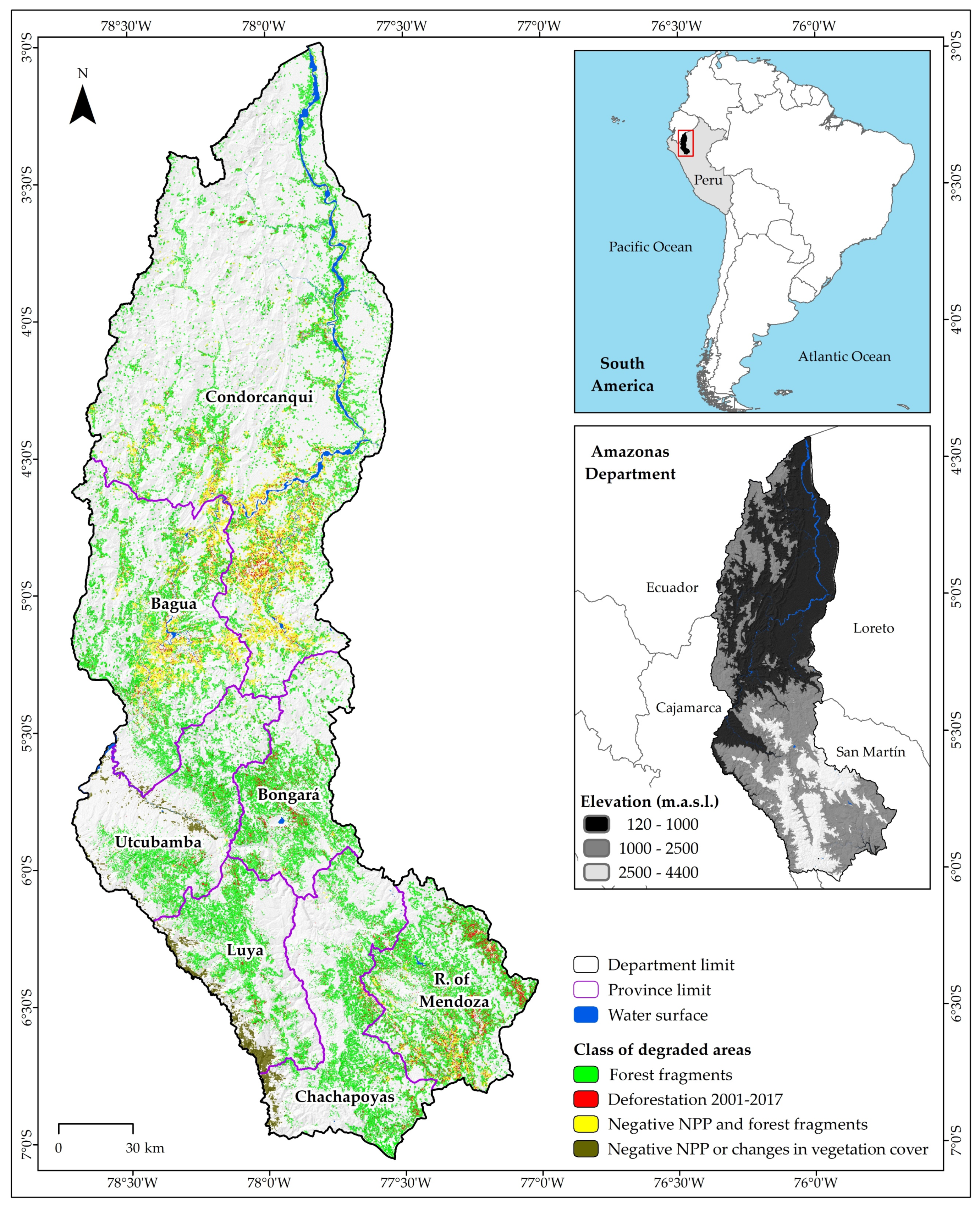
2.1. Study Area

In northeastern Peruvian Andes, the Amazonas Department covers approximately 42050.37 km2 of rugged territory, covered mainly by the Amazon rainforest (Figure 1, 3°0′–7°2′ S, and 77°0′–78°42′ W), along an elevational gradient from 120 m.a.s.l. in the north to 4900 m.a.s.l. in the south. It has contrasting climates (“warm and humid”, “dry warm”, and “warm and slightly humid temperate”), ranging from maximum temperatures of 40 °C in the lowland forest in the north to minimum temperatures of 2 °C in the mountain ranges in the southern boundary; some areas have a water deficit of 924 mm/year and others have a surplus of up to 3000 mm/year [33]. As part of their high biophysical diversity, four ecosystems can be distinguished [34]: (i) lowland forest, (ii) high forest or yunga, (iii) Andean forests and grasslands, and (iv) tropical dry forest. Amazonas is composed of seven provinces (Bagua, Bongará, Chachapoyas, Condorcanqui, Luya, Rodríguez of Mendoza, and Utcubamba), and is characterized by its agricultural activity, which occupies 24.9% of the territory and generates 51.22% of the department GDP [34]. However, due to poor agricultural practices [35,36,37], unsustainable forest use [38], deforestation facilitated by road access [39,40,41], and unregulated urban sprawl, 27.4% (11,533.93 km2) of the Department is degraded territory that has been incorporated into the National Map of Degraded Lands [7]. This map identified four classes of degradation grouped into three categories: “low” (forest fragments, 8638.91 km2), “medium” (negative Net Primary Productivity (NPP) and forest fragments, 1551.45 km2; negative NPP or changes in vegetation cover, 383.13 km2), and “high” (deforestation 2001–2017, 960.45 km2).

2.2. Observed Geographical Records of Forest Species

In order to model the distributions of the species of interest, the five TFS with the highest volume approved for timber harvesting in 2018 in Amazonas were selected [42]. Observed geographic records correspond to trees verified during visual inspections on field trips. These inspections are carried out by the Executive Directorate of Forest and Wildlife Management (DEGBFS) of the Regional Environmental Authority of the Regional Government of Amazonas and informed to the Forest and Wildlife Resources Monitoring Agency (OSINFOR). The complete database is not published, hence the data used here were acquired through: (i) a virtual request to the OSINFOR and (ii) personal coordination with the DEGBFS. In addition, that database was complemented with field records taken between September and October 2018. From the universe of georeferenced records, we discarded records at the genus level and records in which inconsistencies were detected regarding the altitudinal ranges of the species. In sum, 2193, 333, 241, 210, and 215 record points of C. cateniformis, C. pentandra, A. leiocarpa, C. decandra, and C. montana, respectively, were obtained.

2.3. Environmental Variables

The spatial distribution of species within the landscape is due to variables which interact and favor their optimal development [43]. These variables were identified taking into account those reported in the studies on potential distribution [44,45,46] and distribution [47,48,49,50,51] of TFS. In this sense, 26 environmental variables were identified, including 19 bioclimatic variables, solar radiation, 3 topographical variables, and 3 soil chemical properties.
Climate information with a spatial resolution of 30 s (~1 km) was taken from WorldClim (http://worldclim.org). Worldclim’s version 2 [52] was used for bioclimatic information under current conditions (average 1970–2000) and version 1.4 [53] for the periods 2050 (average 2041–2060) and 2070 (average 2061–2080). The four Representative Concentration Pathways (RCP) [54] of the Community Climate System Model version 4 (CCSM4) [55] were considered for 2050 and 2070. Namely, RCPs represents the range of GHG emissions, a scenario with declining radiative level (RCP 2.6), two intermediate scenarios (RCP 4.5 and RCP 6.0), and a very high (RCP 8.5) by 2100 [56]. Indeed, the CCSM4 model is one of the most widely used and efficient global climate projections for predicting changes in plant species distribution [25,28,57,58,59]. The topographic variables were downloaded from a Digital Elevation Model (DEM), 90 m in spatial resolution, from the United States Geological Survey website (http://srtm.usgs.gov). This DEM has been generated based on data from the Shuttle Radar Topography Mission (SRTM) [60]. Soil chemical properties, with a resolution of 250 m, were obtained from the SoilGrids system version 0.5.3 (https://soilgrids.org/) [61]. Non-climate variables (three topographic, three soil properties, and solar radiation) were assumed to be unchanged for 2050 and 2070.
Mapping of environmental variables and species records at a spatial resolution of 250 meters and management of post-modelling spatial information were performed in the open-source GIS software QGIS (version 3.6).

2.4. Environmental Variable Selection

Collinearity between environmental variables may cause over-adjustment problems, and is expected to increase uncertainty and decrease the statistical power of the model [62,63]. Therefore, pixel values were extracted from the 26 thematic layers (environmental variables under current climate) corresponding to the coordinates of the species presence records [64]. Afterwards, the R programming language (version 3.5.2) was used for statistical analysis. We calculated: (i) Pearson’s correlation coefficients (r) between the variables (Tables S1–S5), from which, (ii) the optimal number of clusters was determined using Euclidean distances and the K-means clustering algorithm in the factoextra package and (iii) the cluster dendrogram for each species was constructed (Figures S1–S5) [30]. As a result, nine groups of intercorrelated variables were found for A. leiocarpa, seven for C. decandra, nine for C. montana and ten groups for both C. cateniformis and C. pentandra. In order to obtain a subset of uncorrelated environmental variables for the execution of the models for each species (Table 1), variables with a correlation value of r ≥0.7 were excluded from each group. This threshold is an acceptable measure to minimize the multicollinearity of the adjusted models [62].

2.5. Species Distribution Modelling

Species distribution models for current conditions and for climate change scenarios for each TFS were generated using the machine learning algorithm which applies the principle of Maximum Entropy [18], implemented in the open source software MaxEnt version 3.4.1. Thereby, for each TFS, 75% and 25% of the presence records (selected at random) were used for training and model validation, respectively [18]. The algorithm was run using 10 replicates in 1000 iterations at different random partitions (bootstrap method), a convergence threshold of 0.00001 and 10,000 maximum background points. Other settings were kept to default [29], since MaxEnt is able to select the appropriate function for the number of samples used for a model [21,62]. The models were evaluated using the Area Under the Curve (AUC) statistic [18,65], which is calculated from the Receiver Operating Characteristic (ROC) [66]. According to the AUC values, five levels of performance are differentiated [67]: excellent (>0.9), good (0.8–0.9), accepted (0.7–0.8), poor (0.6–0.7), and unsatisfactory (<0.6). For the current and future models of the five TFS, the logistic output format was used [68]. This format generated a map of continuous probability values for the species distribution, ranging from 0 to 1. These were reclassified into four probability ranges [69]: ‘high’ (>0.6), ‘moderate’ (0.4–0.6), and ‘low’ (0.2–0.4) potential habitat, and the fourth one referred to as ‘non-potential habitat’ (<0.2). These not very restrictive cut-off thresholds were considered, to achieve a larger area and apply a precautionary principle, due to the restoration/conservation objectives of our models [44]. The ‘high’ potential habitats or species distribution were then combined to build combined species distribution maps. These were reclassified into ‘high’, ‘moderate’, and ‘low’ potential habitat, corresponding to areas with 3–5, 2 and 1 species, respectively.

2.6. Identifying Areas with Potential for Forest Restoration

On the basis of the cartographic superposition of three potential distribution ranges (>0.2) under current conditions and the four classes of degradation of the National Map of Degraded Areas [7], cross matrices were constructed. Such matrices allowed the identification of sites with different levels of restoration potential, either with the installation of individual and/or combined species. Areas of high restoration potential and priority are those that resulted from the overlap of the potential distribution of ‘high’ habitat and the ‘Deforestation 2001–2017’ degradation class (corresponding to the ‘high’ degradation category).

3. Results

3.1. Performance of the Species Distribution Models

We have obtained a total of 45 species distribution models, including one under current conditions and eight under climate change scenarios for each TFS. From these results, four of the five TFS had AUC > 0.9 in all their models, showing excellent predictive performance, except the AUC of the C. montana models, which are considered good (0.8 < AUC < 0.9). The mean AUC values of the five TFS varied from 0.864 (C. montana) to 0.962 (A. leiocarpa) having a mean across all species of 0.929 (Table 2).

3.2. Environmental Variables Contributions

Six temperature variables (bio01, annual mean temperature; bio02, mean diurnal range; bio03, isothermality; bio06, min temperature of coldest month; bio09, mean temperature of driest quarter; and bio10, mean temperature of warmest quarter), three precipitation variables (bio16, precipitation of wettest quarter; bio18, precipitation of warmest quarter; and bio19, precipitation of coldest quarter), solar radiation (rad), soil pH (ph), and elevation above mean sea level (dem) appeared to be highly contributing to climatic suitability. In all scenarios, >75% of the potential distribution of each TFS was driven by a combination of only three environmental variables. Namely, 83.7% to 89.2% of the potential distribution of A. leiocarpa was driven by a combination of only three environmental variables between dem, bio18, bio10, and bio16; 83.0% to 93.8% of C. decandra between dem, bio09, bio03, bio10, and bio16; 80.8% to 98.9% of C. montana between bio18, bio19, ph, bio06, and bio02; 75.1% to 88.4% of C. cateniformis between bio09, dem, bio18, and bio3; and 80.0% to 88.8% of C. pentandra between dem, bio01, bio18, and rad.

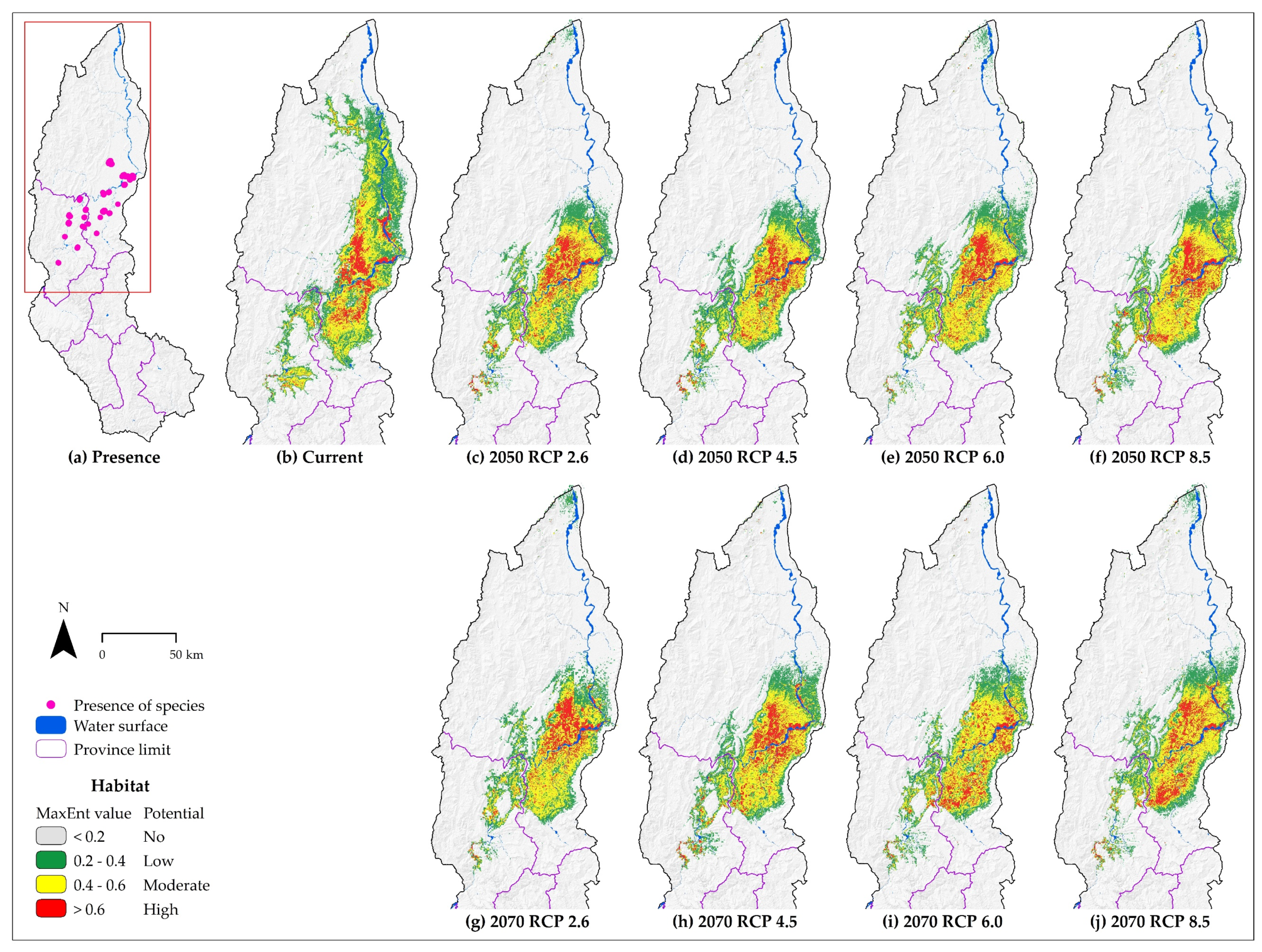
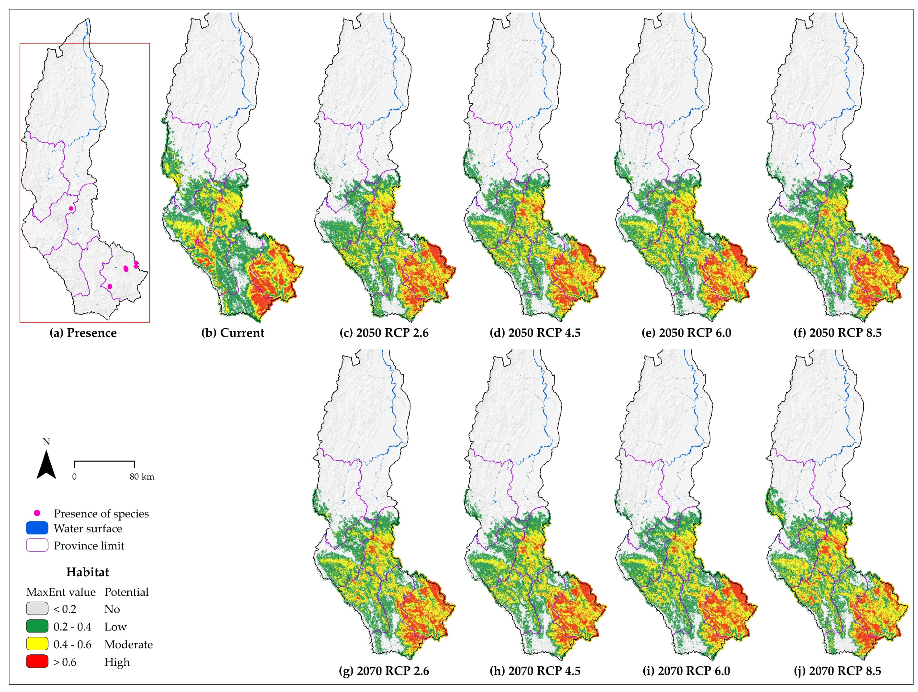
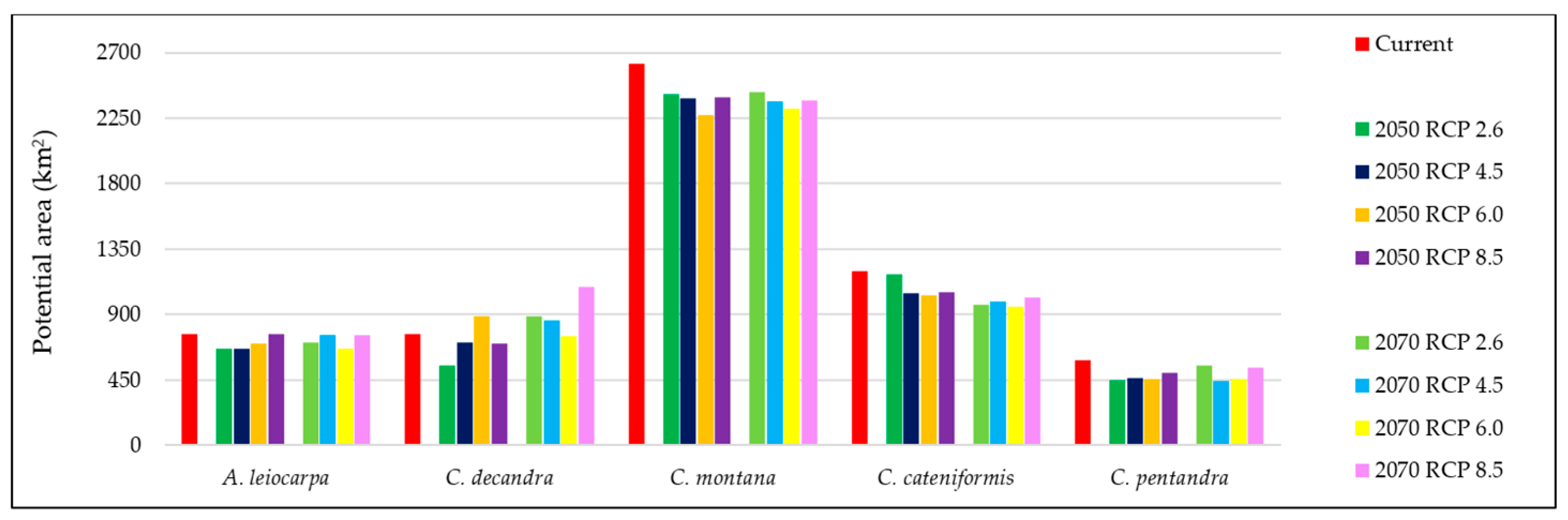
3.3. Species Distribution of Each Species

Under current conditions, C. cateniformis, C. pentandra, A. leiocarpa, and C. decandra are modelled in the northeastern corner of the Amazonas Department (Figure 2, Figure 3, Figure 4 and Figure 5), corresponding to the lowland rainforest ecosystem. This ecosystem registers mean annual temperature between 23–27 °C, annual precipitation between 1800–2440 mm, and altitudinal range of 155–800 m.a.s.l. By 2050 and 2070, potential distribution of C. cateniformis is projected to increase its area, while A. leiocarpa, C. decandra, and C. pentandra are projected to decrease their surface area, with exceptions under certain climate change scenarios. On the other hand, under current conditions, C. montana is modelled in the southeastern of Amazonas Department (Figure 6), in primary vegetation within montane or cloud forests. This ecosystem present habitats with mean annual temperature between 8–20 °C, annual precipitation between 650–1540 mm, and altitudinal range of 1050–3400 m.a.s.l. By 2050 and 2070, potential distribution of C. montana is projected to decrease its area.
Current ‘high’, ‘moderate’, and ‘low’ potential habitat areas in current conditions for C. cateniformis correspond to 2.84% (1194.76 km2), 6.34% (666.85 km2), and 11.31% (4757.6 km2) of Amazonas lands, respectively (Table 3). Taking futures scenarios into consideration, High’ potential habitat is likely to decrease, while ‘moderate’ and ‘low’ potential habitats are expected to increase. On the other side, under current conditions, ‘moderate’ potential habitat will increase by up to 88.88% and 66.9% by 2050 (RCP 4.5) and 2070 (RCP 4.5), respectively.
The areas of current ‘high’, ‘moderate’, and ‘low’ potential habitat in current conditions for C. pentandra correspond to 1.49% (584.39 km2), 5.01% (1966.59 km2), and 7.97% (3128.21 km2) of Amazonas, respectively (Table 3). Those three ranges of distribution will decrease under all future scenarios with respect to the current area. Namely, the potential ‘high’ habitat will decrease by up to −23.7% and −24.2% by 2050 (RCP 2.6) and 2070 (RCP 4.5), respectively. However, based on the surface area in 2050, the ‘high’ potential habitat is likely to increase by up to 23.3% by 2070 (RCP 2.6).
Areas of ‘high’, ‘moderate’, and ‘low’ potential habitat in current conditions for A. leiocarpa correspond to 1.81% (761.55 km2), 5.83% (2449.94 km2), and 6.71% (2822.38 km2) of Amazonas, respectively (Table 3). All three distribution ranges will decrease under all future scenarios with respect to the current area. Namely, the potential ‘high’ habitat will decrease by up to −12.8% and −13.3% by 2050 (RCP 2.6 and RCP 4.5) and 2070 (RCP 6.0), respectively. Based on the surface area in 2050, by 2070 the ‘high’ potential habitat will decrease by up to −9.4% under the CCSM4 RCP 6.0 scenario but increase by up to 14.4% under the CCSM4 RCP 4.5 scenario.
The areas of current ‘high’, ‘moderate’, and ‘low’ potential habitat in current conditions of C. decandra correspond to 1.81% (761.67 km2), 4.48% (1885.82 km2), and 6.90% (2903.42 km2) of Amazonas, respectively (Table 3). With respect to the current suitable area, the three ranges of distribution are expected to decrease under all scenarios by 2050, with the exception of the CCSM4 RCP 6.0 scenario. Namely, the potential ‘high’ habitat will decrease by up to −27.9% under the CCSM4 RCP 2.6 scenario. However, it will increase by up to 16.1% under the CCSM4 RCP 6.0 scenario. There will be an increase and a decrease in potential habitat by 2070 under different ranges and scenarios, compared to the current suitable area and compared to 2050. Namely, the potential ‘high’ habitat under the CCSM4 RCP 8.5 scenario will increase by up to 42.5% and 55.3% over the current area of suitable land and 2050, respectively.
Areas of current ‘high’, ‘moderate’, and ‘low’ potential habitat under current conditions of C. montana correspond to 6.24% (2625.42 km2), 13.87% (5832.68 km2), and 20.57% (8649.03 km2) of Amazonas, respectively (Table 3). The potential ‘high’ habitat will decrease under all future scenarios, with respect to the current suitable area and with respect to 2050 (except under CCSM4 2070 RCP 6.0 scenario for 2070). This means a decrease of by up to −13.4% and −12.0% by 2050 (RCP 6.0) and 2070 (RCP 6.0), respectively, compared to the current suitable area.
Under current conditions, the largest potential ‘high’ habitat areas of 2625.42 km2 and 1194.76 km2, respectively, were modelled for both C. montana and C. cateniformis. The species taking up the smallest area (584.39 km2) of potential ‘high’ habitat is C. pentandra (Figure 7). In such circumstances, by 2050 and 2070, 35 of the 40 models under future scenarios have projected a loss in the area of ‘high’ potential habitat ranging from −0.2 to −27.9% of the current suitable area. However, there is a significant increase in the area of habitat in the remaining five models from 12.7% to 42.5% for C. decandra and 0.2% for A. leiocarpa.

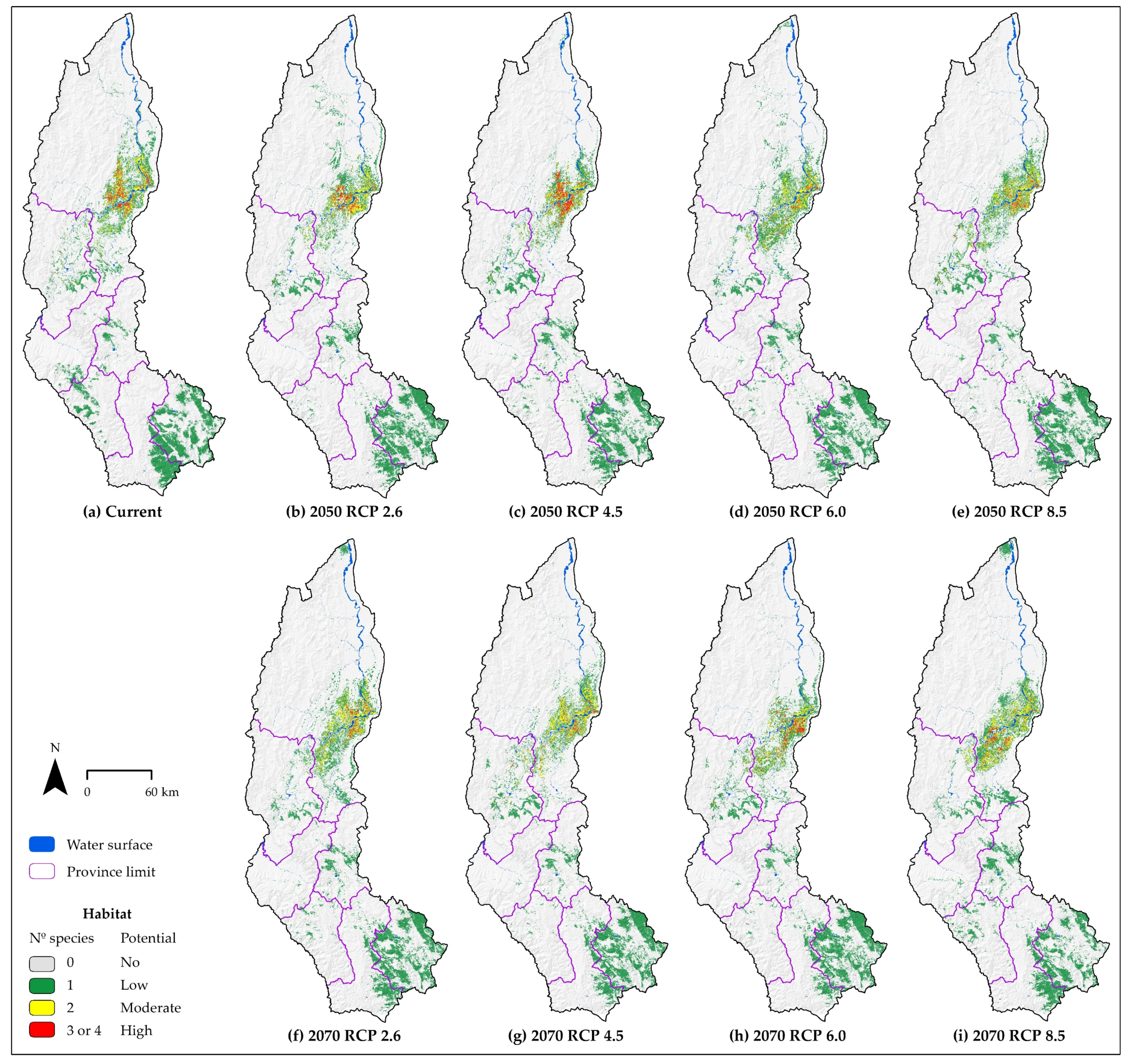
3.4. Combined Species Distribution of Multiple Species

We combined potential distribution of ‘high’ habitat and found that there is no single area hosting five TFS (Figure 8). Therefore, it was reclassified into ‘high’, ‘moderate’, and ‘low’ potential habitat and they correspond to areas with 3 or 4, 2 and 1 species, respectively. Under current conditions and all future scenarios, the concentration region of both ‘high’ and ‘moderate’ potential habitats of the five TFS is modelled to the northeast of Amazonas, in the lowland rainforest ecosystem. On the contrary, habitats with ‘‘low’’ potential are concentrated in the southeast of Amazonas, in primary vegetation within montane or cloud forests. This habitat, which is found in the mountain range, not be suitable for all TFS in almost all future scenarios.
The areas of current ‘high’, ‘moderate’, and ‘low’ potential habitat under current conditions for all five TFS combined correspond to 0.43% (182.26 km2), 1.30% (547.58 km2), and 10.17% (4275.76 km2) of Amazonas, respectively (Table 4). Taking current suitable area into account, the potential ‘high’ habitat will decrease under all future scenarios (except under CCSM4 2050 RPC scenario 4.5). In other words, it will decrease by up to −56.2% and −42.6% by 2050 (RPC 6.0) and 2070 (RPC 4.5), respectively. On the other hand, under the CCSM4 2050 RPC 4.5 scenario it is expected to increase by 30.8%. A better picture is observed regarding suitable area for 2050, the ‘high’ potential habitat will increase by up to 95.0% by 2070 (RPC 6.0).

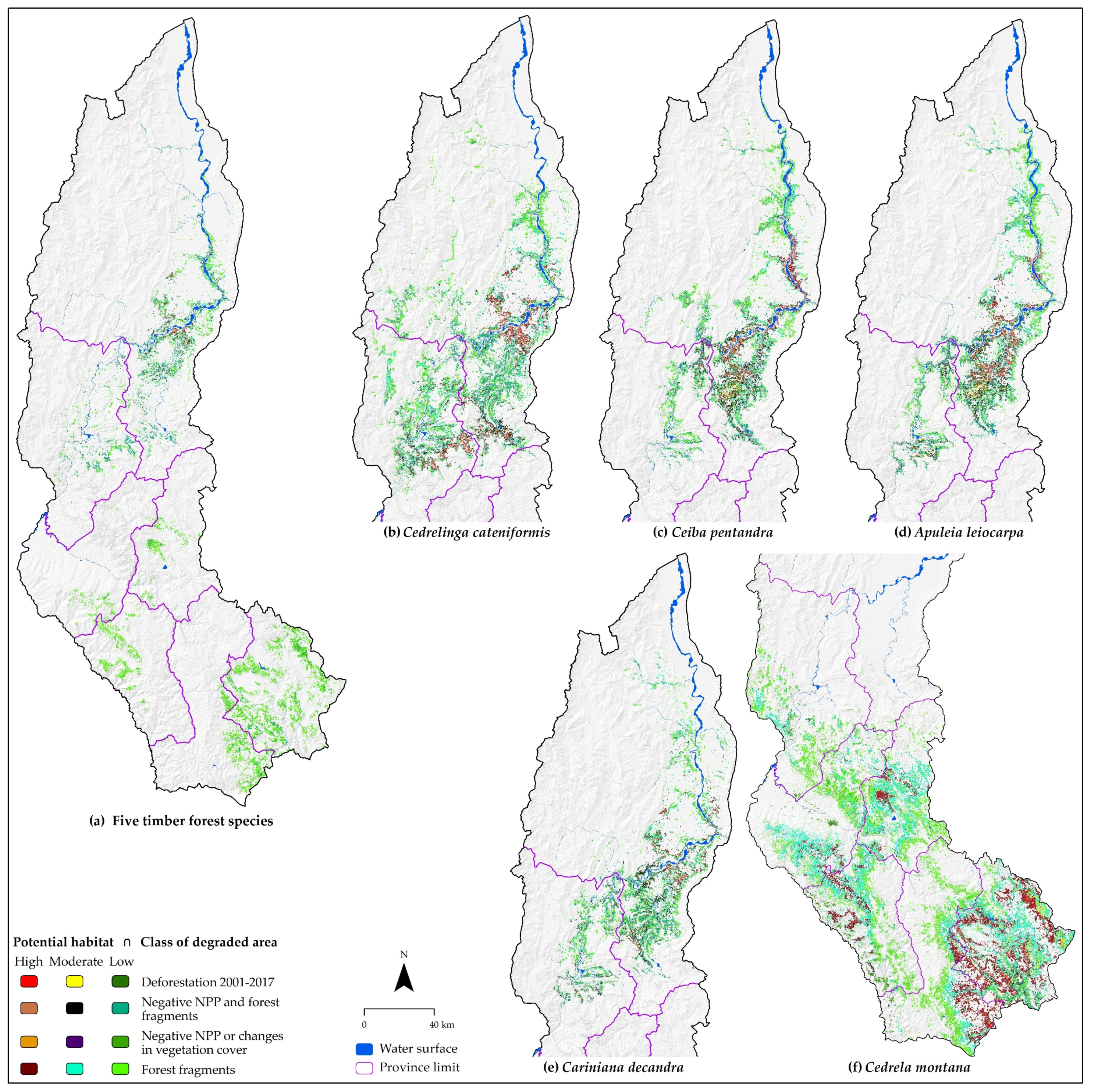
3.5. Degraded Lands with Restoration Potential

Figure 9 shows degraded lands with potential for restoration based on degradation class and current potential habitat range, either with individual species or a combination of multiple species (3 or 4, 2 and 1). Here, C. cateniformis, C. pentandra, A. leiocarpa, and C. decandra have potential for restoration mainly in northeastern Amazonas; while C. montana has potential for restoration in southeastern Amazonas. Of the area of potential ‘high’ habitat under current climate for C. cateniformis, C. pentandra, A. leiocarpa, C. decandra, and C. montana, 3.21% (38.40 km2), 6.58% (38.48 km2), 5.06% (38.56 km2), 1.93% (14.67 km2), and 5.00% (131.27 km2), respectively, were identified to be of high restoration potential (Figure 9b–f; Table 5). Of the ‘high’ potential habitat area under current climate, combination of 3 or 4 species (182.26 km2), only 2.82% (5.14 km2) was identified to have high restoration potential (Figure 9a; Table 5). Over 30% of the total suitability area under the current climate for each species covers degraded areas that can be restored. However, C. montana (6125.44 km2; 35.81% of its total suitability) and C. cateniformis (2985.51 km2; 34.64% of its total suitability) cover the largest degraded areas and thus have potential for restoration using these two species. On the other hand, from highest to lowest, 53.11%, 25.88%, 18.69%, 18.49%, and 16.03% of the total degraded area of the Amazonas department (11,533.93 km2) can be restored with C. montana, C. cateniformis, C. pentandra, A. leiocarpa, and C. decandra.

4. Discussion

4.1. About the Effects of Climate Change

By 2050 and 2070, all five TFS are projected to change their areas of distribution compared to current conditions. In general terms, C. cateniformis is projected to increase its area, while A. leiocarpa, C. decandra, C. montana and C. pentandra are projected to decrease their surface area, with exceptions under certain climate change scenarios. In the literature, it has been estimated that for many TFS the area of their potential distribution increases in climate change scenarios [16,22,26,31,70,71], while for others it decreases [25,31,70,71]. In addition, the literature shows the increase in the species distribution of TFS in some countries and the decreasing trend of the same TFS in other countries [64,72]. Even contrary trends have been reported for the same TFS in the same geographical area, e.g., Picea crassifolia in the Qilian Mountains (China) [57,73] and Cedrela odorata [72,74] in Mexico. However, it should be considered that species distribution models in climate change scenarios should be interpreted with caution, as they may overestimate the decline or increase, by not considering the qualities of the species to adapt in situ to new conditions, or persist outside the conditions in which they have been observed [75,76]. It is unknown the adaptation of the socio-ecological system to future climate scenarios, particularly for those organisms intrinsically linked to forest health and seed dispersal as key agents of restoration [77].
In Peru, the main in situ conservation strategy is the establishment of public and private Protected Areas (PA); these PA usually include important strategies for restoration of degraded lands. Amazonas is one of the regions with the most PAs [78,79]. In this study, the percentage of the species distribution of each TFS within a PA under current conditions and climate change scenarios was not determined. However, future studies could evaluate the effectiveness of the PA network in Amazonas in properly protecting TFS and other species of concern [80]. In case they are determined to be deficient, the government could establish nature conservation areas that cover the species distribution modelled here and reduce human intervention in these areas. Projections reveal that climate change will cause changes in the distribution of TFS. However, the relatively stable distribution sites of each TFS are essential for the sustainable supply of raw materials and environmental services. Therefore, this change in distribution should attract special interest from environmentalists for regenerative development [27]. Although in situ conservation is essential to renew genetic diversity and cope with future environmental changes, ex situ conservation is operationally desirable for short-term results [81]. We suggest that the main ex situ conservation strategy should be the establishment of plantations for restoration in the areas identified in this study [27]. Priority should be given to those areas that are environmentally appropriate for each TFS both in current conditions and in climate change scenarios and those areas that are environmentally appropriate for more than one TFS.

4.2. About Forest Restoration in Peru

More than 30% of the species distribution under current climate of each TFS covers degraded areas and therefore might be restored with the installation of aggressive and proactive restoration strategies with these TFS. These strategies could include afforestation and reforestation of existing remnant patches. Current and future land degradation and deforestation have led to global (see [82,83]) and regional (see [84]) commitments for Forest Landscape Restoration (FLR) [1,85], biodiversity conservation, combating desertification, and mitigation of anthropogenic climate change impacts [8,86]. In Peru, ambitious environmental goals have been set to stop deforestation by 2021 and reduce greenhouse gas emissions caused by land use change [87]. Furthermore, as a country signatory to the Initiative 20 × 20 [84], Peru has committed to reforesting 32,000 km2 of degraded land. In this context, various strategies have been proposed in the area of forestry, including forest policy reform through legislature (Law Nº 29,763 [88]). Although this reform has been criticized [14], in line with this study, Law Nº 29,763 highlights the national strategy to promote forest plantations established on deforested and degraded lands, thus advancing national reforestation objectives and prohibiting logging of natural forests to establish timber plantations [89]. It also seeks to avoid the mechanisms for approving authorization to extract timber from natural forests, namely (a) Forest Management Plan (medium to high intensity, mechanized) and (b) Management Declarations (low intensity, not mechanized). The latter, currently the most widely used, has caused severe damage to forests due to its highly selective nature, altering forest canopy and opening up clearings [90]. The forest roads and clearings are then exploited by migratory agriculture which degrades lands even further [6,39]. Therefore, this study provides a key input for the success of forest plantations, identifying habitats with potential for TFS success. The methodology described here can be applied to more TFS and on a national scale, with the necessary adaptations.
Finally, many forestry projects being implemented by public entities in Amazonas (Regional Agrarian Directorate, Regional Environmental Authority, provincial and district municipalities, etc.) are promoting forest plantations with exotic species such as pine (Pinus sp.), eucalyptus (Eucalyptus sp.), cypress (Cupressus sp.), etc., without taking into account that there are many native tree species [91]. The use of exotic species for afforestation/reforestation is widely practiced in the country, and even many other countries in the region do so. Although there are gaps in the biology and reproduction of native species for plantations, some have been identified as having the potential to be installed in forest plantations [92], forest massifs or agroforestry systems [70], or have been used in restoration initiatives [11]. In 94 restoration experiences in the last 50 years in Peru, the use of native species predominated, considered in turn as the main criterion for the selection of species, followed by the availability of planting material, species useful for correcting degradation and species of commercial interest [11]. Therefore, it is advisable that when designing a forestry project and selecting species, key criteria should be taken into account, such as: (a) each species has its own suitable habitat in which it can be planted, as identified here; (b) first priority should be given to species that are native to a particular area; (c) if there are no native species with the required potential, priority should be given to species from other surrounding areas; and (d) if none of the above are found, exotic species that are already adapted to the area should be proposed. The combination of species distribution models and specific evidence-based management and restoration techniques can certainly be the guide of more successful forestry projects.

5. Conclusions

The species distribution of five TFS in the Amazonas Department, Peru, was successfully modelled under current climate and future climate change scenarios. More than 30% of the species distribution under current climate of each TFS covers degraded areas and therefore may be restored with these TFS. By 2050 and 2070, all five TFS are projected to change their areas of distribution compared to current conditions. In general, C. cateniformis is projected to increase its area, while A. leiocarpa, C. decandra, C. montana, and C. pentandra are projected to decrease their surface area, with exceptions under certain climate change scenarios. Climate change will alter species distribution ranges, which is crucial to understand the spatio-temporal dynamics of TFS species. Current suitable areas should have two strategies to protect the species’ range. One is the conservation prioritization strategy, and the other is the restoration strategy. This study aims to provide maps of potential areas for restoration based on TFS and methodological inputs for the design, implementation and evaluation of restoration initiatives with forest species in Peru; inputs that could also be applied to other restoration initiatives elsewhere. This methodology will guide the economic and ecological success of forest plantations and will allow for the reduction of territory degraded by deforestation or other activities.

Supplementary Materials

The following are available online at https://www.mdpi.com/1424-2818/12/8/305/s1, Figure S1. (a) Pearson’s correlation coefficients (r), (b) Optimal number of clusters and (c) Cluster dendrogram calculated between the environmental variables for the modelling of the potential distribution of A. leiocarpa in Amazonas (Peru), Figure S2. (a) Pearson’s correlation coefficients (r), (b) Optimal number of clusters and (c) Cluster dendrogram calculated between the environmental variables for the modelling of the potential distribution of C. decandra in Amazonas (Peru), Figure S3. (a) Pearson’s correlation coefficients (r), (b) Optimal number of clusters and (c) Cluster dendrogram calculated between the environmental variables for the modelling of the potential distribution of C. montana in Amazonas (Peru), Figure S4. (a) Pearson’s correlation coefficients (r), (b) Optimal number of clusters and (c) Cluster dendrogram calculated between the environmental variables for the modelling of the potential distribution of C. cateniformis in Amazonas (Peru), Figure S5. (a) Pearson’s correlation coefficients (r), (b) Optimal number of clusters and (c) Cluster dendrogram calculated between the environmental variables for the modelling of the potential distribution of C. pentandra in Amazonas (Peru), Table S1. Pearson’s correlation coefficients (r) calculated between the environmental variables for the modelling of the potential distribution of A. leiocarpa in Amazonas (Peru), Table S2. Pearson’s correlation coefficients (r) calculated between the environmental variables for the modelling of the potential distribution of C. decandra in Amazonas (Peru), Table S3. Pearson’s correlation coefficients (r) calculated between the environmental variables for the modelling of the potential distribution of C. montana in Amazonas (Peru), Table S4. Pearson’s correlation coefficients (r) calculated between the environmental variables for the modelling of the potential distribution of C. cateniformis in Amazonas (Peru), Table S5. Pearson’s correlation coefficients (r) calculated between the environmental variables for the modelling of the potential distribution of C. pentandra in Amazonas (Peru).

Author Contributions

Conceptualization, N.B.R.B., E.B.C. and R.S.L.; Data curation, N.C.R.B., E.B.C. and R.S.L.; Formal analysis, N.B.R.B.; Funding acquisition, M.Á.B.G. and M.O.; Investigation, N.B.R.B., D.A.C.S., E.B.C., D.A.S. and R.S.L.; Methodology, N.B.R.B., D.A.C.S., E.B.C., F.O.S., D.A.S. and R.S.L.; Project administration, M.Á.B.G., M.O. and R.S.L.; Software, N.B.R.B., D.A.C.S., D.A.S. and R.S.L.; Supervision, M. Á.B.G., F.O.S., M.O. and R.S.L.; Validation, M.Á.B.G. and F.O.S.; Visualization, M.Á.B.G. and M.O.; Writing—original draft, N.B.R.B.; Writing—review & editing, N.B.R.B., E.B.C., M.Á.B.G., F.O.S., D.A.S., M.O. and R.S.L. All authors have read and agreed to the published version of the manuscript.

Funding

This work was carried out with the support of the Public Investment Projects CEINFOR (SNIP No. 352650) and GEOMATICA (SNIP No. 312235), executed by the Cloud Forest’s Sustainable Development Research Institute (INDES-CES) of the National University Toribio Rodríguez of Mendoza (UNTRM).

Acknowledgments

The authors acknowledge and appreciate the support of the Research Institute for the Sustainable Development of the Jungle brow zone (INDES-CES) of the National University Toribio Rodríguez of Mendoza (UNTRM), La Molina National Agrarian University, and the Neotropical Montology Collaboratory of the University of Georgia.

Conflicts of Interest

The authors declare no conflict of interest.

References

  1. Sabogal, C.; Besacier, C.; McGuire, D. Forest and landscape restoration: Concepts, approaches and challenges for implementation. Unasylva 2015, 66, 3–10. [Google Scholar]
  2. FAO. Evaluación de los recursos forestales mundiales 2015. In ¿Cómo Están Cambiando Los Bosques Del Mundo? 2nd ed.; FAO: Roma, Italia, 2016; ISBN 9789253092833. [Google Scholar]
  3. MINAM. GEOBOSQUES: Bosque y Pérdida de Bosque. Available online: http://geobosques.minam.gob.pe/geobosque/view/perdida.php (accessed on 15 December 2019).
  4. De Sy, V.; Herold, M.; Achard, F.; Beuchle, R.; Clevers, J.G.P.W.; Lindquist, E.; Verchot, L. Land use patterns and related carbon losses following deforestation in South America. Environ. Res. Lett. 2015, 10, 124004. [Google Scholar] [CrossRef]
  5. Guariguata, R.M.; Arce, J.; Ammour, T.; Capella, J.L. Las Plantaciones Forestales en Perú: Reflexiones, Estatus Actual y Perspectivas a Futuro; CIFOR: Bogor, Indonesia, 2017; ISBN 9786023870530. [Google Scholar]
  6. Dourojeanni, R.M.J. Aprovechamiento del barbecho forestal en áreas de agricultura migratoria en la Amazonía peruana. Revi. For. Perú 1987, 14, 1–33. [Google Scholar] [CrossRef]
  7. MINAM. Estudio para la Identificación de Áreas Degradadas y Propuesta de Monitoreo; MINAM: Lima, Perú, 2017.
  8. Román, F.; Mamani, A.; Cruz, A.; Sandoval, C.; Cuesta, F. Orientaciones Para la restauracion de ecosistemas forestales y otros ecosistemas de vegetación Silvestre; SERFOR: Lima, Perú, 2018. [Google Scholar]
  9. Laestadius, L.; Maginnis, S.; Minnemeyer, S.; Potapov, P.; Saint-Laurent, C.; Sizer, N. Mapa de oportunidades de restauración del paisaje forestal. Unasylva 2011, 62, 47–48. [Google Scholar]
  10. Hillbrand, A.; Borelli, S.; Conigliaro, M.; Olivier, A. Agroforestry for Landscape Restoration: Exploring the Potential of Agroforestry to Enhance the Sustainability and Resilience of Degraded Landscapes; FAO: Rome, Italy, 2017. [Google Scholar]
  11. Cerrón, M.J.; del Castillo, R.J.D.; Thomas, E.; Mathez-Stiefel, S.-L.; Franco, C.M.; Mamani, C.A.; González, C.F.B.I. Experiencias de restauración en el Perú: Lecciones aprendidas; SERFOR: Bioversity, Perú; ICRAF: Lima, Perú, 2018; ISBN 9786124690839. [Google Scholar]
  12. Berrahmouni, N.; Regato, P.; Perfondry, M. Global Guidelines for the Restoration of Degraded Forests and Landscapes in Drylands: Building Resilience and Benefitting Livelihoods; FAO: Roma, Italia, 2015; Volume 25, ISBN 9789251089125. [Google Scholar]
  13. Sarmiento, F. Restoration of Equatorial Andes: The challenge for conservation of tropandean landscapes. In Biodiversity and Conservation of Neotropical Montane Forests; Churchill, S., Balslev, H., Forero, E., Luteyn, J., Eds.; The New York Botanical Garden: Nueva York, NY, USA, 1995; pp. 637–651. [Google Scholar]
  14. Dourojeanni, M.J. Esbozo de una nueva política forestal peruana. Rev. For. Perú 2019, 34, 4. [Google Scholar] [CrossRef]
  15. Sarmiento, F. Arrested succession in pastures hinders regeneration of Tropandean forests and shreds mountain landscapes. Environ. Conserv. 1997, 24, 14–23. [Google Scholar] [CrossRef]
  16. Xu, X.; Zhang, H.; Yue, J.; Xie, T.; Xu, Y.; Tian, Y. Predicting shifts in the suitable climatic distribution of walnut (Juglans regia L.) in China: Maximum entropy model paves the way to forest management. Forests 2018, 9, 103. [Google Scholar] [CrossRef] [Green Version]
  17. Mateo, R.G.; Felicísimo, Á.M.; Muñoz, J. Modelos de distribución de especies: Una revisión sintética. Rev. Chil. Hist. Nat. 2011, 84, 217–240. [Google Scholar] [CrossRef] [Green Version]
  18. Phillips, S.J.; Anderson, R.P.; Schapire, R.E. Maximum entropy modeling of species geographic distributions. Ecol. Model. 2006, 190, 231–252. [Google Scholar] [CrossRef] [Green Version]
  19. Hernandez, P.A.; Graham, C.H.; Master, L.L.; Albert, D.L. The effect of sample size and species characteristics on performance of different species distribution modeling method. Ecography 2006, 29, 773–785. [Google Scholar] [CrossRef]
  20. Aguirre-Gutiérrez, J.; Carvalheiro, L.G.; Polce, C.; van Loon, E.E.; Raes, N.; Reemer, M.; Biesmeijer, J.C. Fit-for-Purpose: Species Distribution Model Performance Depends on Evaluation Criteria-Dutch Hoverflies as a Case Study. PLoS ONE 2013, 8, e0063708. [Google Scholar] [CrossRef] [PubMed] [Green Version]
  21. Merow, C.; Smith, M.J.; Silander, J.A. A practical guide to MaxEnt for modeling species’ distributions: What it does, and why inputs and settings matter. Ecography 2013, 36, 1058–1069. [Google Scholar] [CrossRef]
  22. Bai, Y.; Wei, X.; Li, X. Distributional dynamics of a vulnerable species in response to past and future climate change: A window for conservation prospects. Peer-Rev. J. 2018, 2018, 1–25. [Google Scholar] [CrossRef]
  23. Cavalcante, R.A.; Nascimento, F.A.; Pereira, M.A.; Souza, D.P.; Fontana, A.P.; Cotarelli, V.M.; Oliveira, M.A.; Moura Júnior, E.G. Ampliação do conhecimento biogeográfico de Pleurophora pulchra (Lythraceae) com enfoque da conservação. Rodriguésia 2019, 70, 2–11. [Google Scholar] [CrossRef] [Green Version]
  24. Vilchez, D.; Sotomayor, D.A.; Zorrilla, C. Ex situ conservation priorities for the peruvian wild tomato species (Solanum, L. SECT. Lycopersicum (MILL.) WETTST.). Ecol. Apl. 2019, 18, 171. [Google Scholar] [CrossRef]
  25. Alfonso-Corrado, C.; Naranjo-Luna, F.; Clark-Tapia, R.; Campos, J.E.; Rojas-Soto, O.R.; Luna-Krauletz, M.D.; Bodenhorn, B.; Gorgonio-Ramírez, M.; Pacheco-Cruz, N. Effects of environmental changes on the occurrence of Oreomunnea mexicana (Juglandaceae) in a biodiversity hotspot cloud forest. Forests 2017, 8, 261. [Google Scholar] [CrossRef]
  26. Qin, A.; Liu, B.; Guo, Q.; Bussmann, R.W.; Ma, F.; Jian, Z.; Xu, G.; Pei, S. Maxent modeling for predicting impacts of climate change on the potential distribution of Thuja sutchuenensis Franch., an extremely endangered conifer from southwestern China. Glob. Ecol. Conserv. 2017, 10, 139–146. [Google Scholar] [CrossRef]
  27. Romero-Sanchez, M.E.; Perez-Miranda, R.; Gonzalez-Hernandez, A.; Velasco-Garcia, M.V.; Velasco-Bautista, E.; Flores, A. Current and potential spatial distribution of six endangered pine species of Mexico: Towards a conservation strategy. Forests 2018, 9, 767. [Google Scholar] [CrossRef] [Green Version]
  28. Abdelaal, M.; Fois, M.; Fenu, G.; Bacchetta, G. Using MaxEnt modeling to predict the potential distribution of the endemic plant Rosa arabica Crép. In Egypt. Ecol. Inform. 2019, 50, 68–75. [Google Scholar] [CrossRef]
  29. Otieno, B.A.; Nahrung, H.F.; Steinbauer, M.J. Where did you come from? Where did you go? Investigating the origin of invasive Leptocybe species using distribution modelling. Forests 2019, 10, 115. [Google Scholar] [CrossRef] [Green Version]
  30. Kariyawasam, C.S.; Kumar, L.; Ratnayake, S.S. Invasive plant species establishment and range dynamics in Sri Lanka under climate change. Entropy 2019, 21, 571. [Google Scholar] [CrossRef] [Green Version]
  31. Antúnez, P.; Suárez-Mota, M.E.; Valenzuela-Encinas, C.; Ruiz-Aquino, F. The potential distribution of tree species in three periods of time under a climate change scenario. Forests 2018, 9, 628. [Google Scholar] [CrossRef] [Green Version]
  32. Frey, G.P.; West, T.A.P.; Hickler, T.; Rausch, L.; Gibbs, H.K.; Börner, J. Simulated impacts of soy and infrastructure expansion in the Brazilian Amazon: A maximum entropy approach. Forests 2018, 9, 600. [Google Scholar] [CrossRef] [Green Version]
  33. Vargas, R.; Clima, J. Estudios temáticos para la Zonificación Ecológica Económica del departamento de Amazonas; Instituto de Investigaciones de la Amazonía Peruana (IIAP) & Programa de Investigaciones en Cambio Climático, Desarrollo Territorial y Ambiente (PROTERRA): Chachapoyas, Perú, 2010; Volume 1, pp. 1–27. [Google Scholar]
  34. GRA; IIAP. Zonificación Ecológica y Económica (ZEE) del departamento de Amazonas; GRA and IIAP: Iquitos, Perú, 2010. [Google Scholar]
  35. Oliva, C.S.M.; Maicelo, Q.J.L.; Torres, G.C.; Bardales, E.W. Propiedades fisicoquímicas del suelo en diferentes estadios de la agricultura migratoria en el Área de Conservación Privada “Palmeras de Ocol”, distrito de Molinopampa, provincia de Chachapoyas (departamento de Amazonas). Rev. Investig. Agroproducción sustentable 2017, 1, 9–21. [Google Scholar]
  36. Oliva, C.S.M.; Collazos, S.R.; Espárraga, E.T.A. Efecto de las plantaciones de Pinus patula sobre las características fisicoquímicas de los suelos en áreas altoandinas de la región Amazonas. Rev. INDES 2014, 2, 28–36. [Google Scholar]
  37. Oliva, C.M.; Collazos, S.R.; Goñas, M.M.; Bacalla, E.; Vigo, M.C.; Vásquez, P.H.; Espinosa, L.S.T.; Maicelo, Q.J.L. Efecto de los sistemas de producción sobre las características físico-químicas de los suelos del distrito de Molinopampa, provincia de Chachapoyas, región Amazonas. Rev. INDES 2014, 2, 44–52. [Google Scholar]
  38. Shanee, N.; Shanee, S. Land Trafficking, Migration, and Conservation in the “No-Man’s Land” of Northeastern Peru. Trop. Conserv. Sci. 2016, 9. [Google Scholar] [CrossRef] [Green Version]
  39. Rojas, B.N.B.; Barboza, C.E.; Maicelo, Q.J.L.; Oliva, C.S.M.; Salas, L.R. Deforestación en la Amazonía peruana: Índices de cambios de cobertura y uso del suelo basado en SIG. Boletín De La Asociación De Geógrafos Españoles 2019, 81, 1–34. [Google Scholar] [CrossRef]
  40. Mendoza, C.M.E.; Salas, L.R.; Barboza, C.E. Análisis multitemporal de la deforestación usando la clasificación basada en objetos, distrito de Leymebamba (Perú). Rev. INDES 2015, 3, 67–76. [Google Scholar] [CrossRef] [Green Version]
  41. Salas, L.R.; Barboza, C.E.; Oliva, C.M. Dinámica multitemporal de índices de deforestación en el distrito de Florida, departamento de Amazonas, Perú. Rev. INDES 2014, 2, 18–27. [Google Scholar]
  42. OSINFOR. Reportes Estadísticos: Principales Especies Forestales Maderables Aprobadas. Available online: https://observatorio.osinfor.gob.pe/Estadisticas/Home/Reportes/1 (accessed on 15 December 2019).
  43. Stevens, G.C. The latitudinal gradient in geographic range: How so many species coexist in the tropics. Am. Nat. 1989, 133, 240–256. [Google Scholar] [CrossRef]
  44. OSINFOR. Modelamiento de la distribución potencial de 18 especies forestales en el departamento de Loreto; OSINFOR: Lima, Peru, 2016; ISBN 9786124706028.
  45. OSINFOR. Modelamieto espacial de nichos ecológicos para la evaluación de presencia de especies forestales maderables en la Amazonía Peruana; OSINFOR: Lima, Perú, 2013.
  46. Figueiredo, S.M.D.M.; Venticinque, E.M.; Figueiredo, E.O.; Ferreira, E.J.L. Predição da distribuição de espécies florestais usando variáveis topográficas e de índice de vegetação no leste do Acre, Brasil. Acta Amaz. 2015, 45, 167–174. [Google Scholar] [CrossRef] [Green Version]
  47. OSINFOR. Distribución de las Especies Forestales del Perú; OSINFOR: Lima, Perú, 2013; ISBN 9788578110796.
  48. Pennington, T.; Muellner, A.N.; Wise, R. A Monograph of Cedrela (Meliaceae); Dh Books: Milborne Port, UK, 2010; ISBN 9780953813476. [Google Scholar]
  49. Reynel, C.; Pennington, T.D.; Pennington, R.T. Árboles del Perú; Imprenta Bellido: Lima, Perú, 2016; ISBN 9786120022320. [Google Scholar]
  50. Reynel, C.; Pennington, R.T.; Pennington, T.D.; Flores, C.; Daza, A. Arboles útiles de la Amazonía peruana; Tarea Grafica Educativa: Lima, Perú, 2003. [Google Scholar]
  51. Brako, L.; Zaruchi, J. Catalogue of the Flowering Plants and Gymnosperms of Peru; Missouri Botanical Garden: St. Louis, MO, USA, 1993. [Google Scholar]
  52. Fick, S.E.; Hijmans, R.J. WorldClim 2: New 1-km spatial resolution climate surfaces for global land areas. Int. J. Climatol. 2017, 37, 4302–4315. [Google Scholar] [CrossRef]
  53. Hijmans, R.J.; Cameron, S.E.; Parra, J.L.; Jones, P.G.; Jarvis, A. Very high resolution interpolated climate surfaces for global land areas. Int. J. Climatol. 2005, 25, 1965–1978. [Google Scholar] [CrossRef]
  54. Pachauri, R.K.; Allen, M.R.; Barros, V.R.; Broome, J.; Cramer, W.; Christ, R.; Church, J.A.; Clarke, L.; Dahe, Q.; Dasgupta, P.; et al. Climate Change 2014: Synthesis Report. Contribution of Working Groups I, II and III to the Fifth Assessment Report of the Intergovernmental Panel on Climate Change; IPCC: Geneva, Switzerland, 2014; ISBN 9789291691432. [Google Scholar]
  55. Gent, P.R.; Danabasoglu, G.; Donner, L.J.; Holland, M.M.; Hunke, E.C.; Jayne, S.R.; Lawrence, D.M.; Neale, R.B.; Rasch, P.J.; Vertenstein, M.; et al. The community climate system model version 4. J. Clim. 2011, 24, 4973–4991. [Google Scholar] [CrossRef]
  56. van Vuuren, D.P.; Edmonds, J.; Kainuma, M.; Riahi, K.; Thomson, A.; Hibbard, K.; Hurtt, G.C.; Kram, T.; Krey, V.; Lamarque, J.F.; et al. The representative concentration pathways: An overview. Clim. Chang. 2011, 109, 5–31. [Google Scholar] [CrossRef]
  57. Rong, Z.; Zhao, C.; Liu, J.; Gao, Y.; Zang, F.; Guo, Z.; Mao, Y.; Wang, L. Modeling the effect of climate change on the potential distribution of Qinghai spruce (Picea crassifolia Kom.) in Qilian Mountains. Forests 2019, 10, 62. [Google Scholar] [CrossRef] [Green Version]
  58. Al-Qaddi, N.; Vessella, F.; Stephan, J.; Al-Eisawi, D.; Schirone, B. Current and future suitability areas of kermes oak (Quercus coccifera L.) in the Levant under climate change. Reg. Environ. Chang. 2017, 17, 143–156. [Google Scholar] [CrossRef]
  59. Mousaei, S.M.; Rundel, P.W. The impact of climate change on habitat suitability for Artemisia sieberi and Artemisia aucheri (Asteraceae)—A modeling approach. Pol. J. Ecol. 2017, 65, 97–109. [Google Scholar] [CrossRef]
  60. Farr, T.G.; Rosen, P.A.; Caro, E.; Crippen, R.; Duren, R.; Hensley, S.; Kobrick, M.; Paller, M.; Rodriguez, E.; Roth, L.; et al. The Shuttle Radar Topography Mission. Rev. Geophys. 2007, 45, 1–33. [Google Scholar] [CrossRef] [Green Version]
  61. Hengl, T.; De Jesus, J.M.; Heuvelink, G.B.M.; Gonzalez, M.R.; Kilibarda, M.; Blagotić, A.; Shangguan, W.; Wright, M.N.; Geng, X.; Bauer-Marschallinger, B.; et al. SoilGrids250m: Global gridded soil information based on machine learning. PLoS ONE 2017, 12, e0169748. [Google Scholar] [CrossRef] [PubMed] [Green Version]
  62. Dormann, C.F.; Elith, J.; Bacher, S.; Buchmann, C.; Carl, G.; Carré, G.; García, M.J.R.; Gruber, B.; Lafourcade, B.; Leitão, P.J.; et al. Collinearity: A review of methods to deal with it and a simulation study evaluating their performance. Ecography 2013, 36, 027–046. [Google Scholar] [CrossRef]
  63. De Marco, J.P.; Corrêa, N.C. Evaluating collinearity effects on species distribution models: An approach based on virtual species simulation. PLoS ONE 2018, 13, e02022403. [Google Scholar] [CrossRef] [PubMed]
  64. Laurente, M. Modeling the Effects of Climate Change on the Distribution of Cedrela odorata L. «Cedro» in the Peruvian Amazon. Biology 2015, 13, 213–224. [Google Scholar]
  65. Manel, S.; Ceri, W.H.; Ormerod, S.J. Evaluating presence–absence models in ecology: The need to account for prevalence. J. Appl. Ecol. 2001, 38, 921–931. [Google Scholar] [CrossRef]
  66. Hanley, J.A.; McNeil, B.J. The meaning and use of the area under a receiver operating characteristic (ROC) curve. Radiology 1982, 143, 29–36. [Google Scholar] [CrossRef] [Green Version]
  67. Araujo, M.; Pearson, R.; Thuiller, W.; Erhard, M. Validation of species-climate impact models under climate change. Glob. Chang. Biol. 2005, 11, 1504–1513. [Google Scholar] [CrossRef] [Green Version]
  68. Phillips, S.J.; Dudík, M. Modeling of species distributions with Maxent: New extensions and a comprehensive evaluation. Ecography 2008, 31, 161–175. [Google Scholar] [CrossRef]
  69. Zhang, K.; Zhang, Y.; Tao, J. Predicting the potential distribution of Paeonia veitchii (Paeoniaceae) in China by incorporating climate change into a maxent model. Forests 2019, 10, 190. [Google Scholar] [CrossRef] [Green Version]
  70. Leguía, E.; Soudre, M.; Rugnitz, M. Predicción y evaluación del impacto del cambio climático sobre los sistemas agroforestales en la amazonia peruana y andina ecuatoriana; IIAP, ICRAF: Pucallpa, Perú, 2010. [Google Scholar]
  71. Guzmán, M.A.N.; Chipana, C.A.J.; Apaza, J.M.I. Modeling ecological niches of threatened flora for climate change scenarios in Tacna department-Peru. Colomb. For. 2020, 23. [Google Scholar] [CrossRef]
  72. Estrada-Contreras, I.; Equihua, M.; Laborde, J.; Meyer, E.M.; Sanchez-Velasquez, L.R. Current and future distribution of the tropical tree Cedrela Odorata L. in Mexico under Climate Change Scenarios Using Maxlike. PLoS ONE 2016, 11, e0164178. [Google Scholar] [CrossRef] [PubMed]
  73. Xu, Z.; Zhao, C.; Feng, Z. A study of the impact of climate change on the potential distribution of Qinghai spruce (Picea crassifolia) in Qilian Mountains. Acta Ecol. Sin. 2009, 29, 278–285. [Google Scholar] [CrossRef]
  74. Ramos, J.H.; Santos, R.R.; Ramos, A.H.; Cuevas, X.G.; Hernández-Máximo, E.; Uicab, J.V.C.; López, D.S. Historical, current and future distribution of Cedrela odorata in Mexico. Acta Bot. Mex. 2018, 2018, 117–134. [Google Scholar] [CrossRef]
  75. Lamont, B.B.; Connell, S.W. Biogeography of Banksia in southwestern Australia. J. Biogeogr. 1996, 23, 295–309. [Google Scholar] [CrossRef]
  76. Sarmiento, F.O.; Kooperman, G.J. A Socio-Hydrological Perspective on Recent and Future Precipitation Changes Over Tropical Montane Cloud Forests in the Andes. Front. Earth Sci. 2019, 7, 1–6. [Google Scholar] [CrossRef]
  77. Sarmiento, F.O. Landscape Regeneration by Seeds and Successional Pathways to Restore Fragile Tropandean Slopelands. Mt. Res. Dev. 1997, 17, 239. [Google Scholar] [CrossRef] [Green Version]
  78. SERNANP. Servicio Nacional de Áreas Naturales Protegidas por el Estado. Servicios y Recursos. Available online: https://www.geoidep.gob.pe/servicio-nacional-de-areas-naturales-protegidas-por-el-estado (accessed on 15 April 2019).
  79. SPDA. Áreas de conservación privada en el Perú: Anances y propuestas a 20 años de su creación; Monteferri, B., Ed.; Sociedad Peruana de Derecho Ambiental: Lima, Perú, 2019; ISBN 9786124261442. [Google Scholar]
  80. Salinas-Rodríguez, M.M.; Sajama, M.J.; Gutiérrez-Ortega, J.S.; Ortega-Baes, P.; Estrada-Castillón, A.E. Identification of endemic vascular plant species hotspots and the effectiveness of the protected areas for their conservation in Sierra Madre Oriental, Mexico. J. Nat. Conserv. 2018, 46, 6–27. [Google Scholar] [CrossRef]
  81. Rong-Cai, Y.; Yeh, F.C. Genetic consequences of in situ and ex situ conservation of forest trees. For. Chron. 1992, 68, 720–729. [Google Scholar]
  82. Bonn Challenge. A Global Effort to Bring 150 Million Hectares of Deforested and Degraded Land into Restoration by 2020 and 350 Million Hectares by 2030. Available online: https://www.bonnchallenge (accessed on 24 March 2020).
  83. CBD. Decision Adopted By the Conference of the Parties to the Convention on Biological Diversity at Its Seventh Meeting: XI/16. Ecosystem restoration. In Proceedings of the Conference of the Parties to the Convention on Biological Diversity, Pyeongchang, Korea, 6–17 October 2014; Convention on Biological Diversity: Hyderabad, India, 2012. [Google Scholar]
  84. Initiative 20 × 20. Healthy Lands for Food, Water and Climate. A Country-Led Effort that Aims to Change the Dynamics of Land Degradation in Latin America and the Caribbean. Available online: https://initiative20x20 (accessed on 24 March 2020).
  85. International Union for Conservation of Nature. Forest Landscape Restoration. Available online: https://www.iucn:theme/forests/our-work/forest-landscape-restoration (accessed on 24 March 2020).
  86. Holl, K.D. Restoring tropical forests from the bottom up: How can ambitious forest restoration targets be implemented on the ground? Science 2017, 355, 455–456. [Google Scholar] [CrossRef] [Green Version]
  87. MINAM. Plan Nacional De Acción Ambiental-Planaa Perú: 2011–2021, 2nd ed.; MINAM: Lima, Perú, 2011.
  88. SERFOR. Ley Forestal y de Fauna Silvestre N 29763 y sus reglamentos, 2nd ed.; SERFOR: Lima, Perú, 2015. [Google Scholar]
  89. Sears, R.R.; Cronkleton, P.; Polo Villanueva, F.; Miranda Ruiz, M.; Pérez-Ojeda del Arco, M. Farm-forestry in the Peruvian Amazon and the feasibility of its regulation through forest policy reform. For. Policy Econ. 2018, 87, 49–58. [Google Scholar] [CrossRef]
  90. Mackey, B.; Kormos, C.F.; Keith, H.; Moomaw, W.R.; Houghton, R.A.; Mittermeier, R.A.; Hole, D.; Hugh, S. Understanding the importance of primary tropical forest protection as a mitigation strategy. Mitig. Adapt. Strateg. Glob. Chang. 2020. [Google Scholar] [CrossRef] [Green Version]
  91. Mostacero-Leon, J.; Mejia-Coico, F.; Pelaez-Pelaez, F.; Charcape-Ravelo, M. Especies madereras nativas del norte del perú. Rebiol 1998, 16, 67–78. [Google Scholar]
  92. Baluarte, V.J.R.; Alvarez, G.J.G. Modelamiento del crecimiento de tornillo Cedrelinga catenaeformis Ducke en plantaciones en Jenaro Herrera, departamento de Loreto, Perú. Folia Amaz. 2015, 24, 21. [Google Scholar] [CrossRef] [Green Version]
Figure 1. Location and degraded areas of the Amazonas Department, in the northeast of Peru.
Diversity 12 00305 g001
Figure 2. Potential species distribution under current conditions and climate change scenarios of C. cateniformis in Amazonas (Peru).
Diversity 12 00305 g002
Figure 3. Potential species distribution under current conditions and climate change scenarios of C. pentandra in Amazonas (Peru).
Diversity 12 00305 g003
Figure 4. Potential species distribution under current conditions and climate change scenarios of A. leiocarpa in Amazonas (Peru).
Diversity 12 00305 g004
Figure 5. Potential species distribution under current conditions and climate change scenarios of C. decandra in Amazonas (Peru).
Diversity 12 00305 g005
Figure 6. Potential species distribution under current conditions and climate change scenarios of C. montana in Amazonas (Peru).
Diversity 12 00305 g006
Figure 7. Potential distribution of ‘high’ habitat under current conditions and climate change scenarios of five TFS in Amazonas (Peru). In order to analyze the variation in area for each species, the current scenario should be compared with the same climate change scenario (RCP) in 2050 (i.e., RCP 2.6) and 2070 (i.e., RCP 2.6).
Diversity 12 00305 g007
Figure 8. Combined potential distribution of ‘high’ habitat under current conditions and climate change scenarios of five TFS in Amazonas (Peru).
Diversity 12 00305 g008
Figure 9. Degraded lands with potential for restoration based on the species distribution of five separated or combined TFS in current conditions in Amazonas (Peru). In the legend, the color red (top left) denotes areas with high potential and restoration priority, the color green (bottom right) represents areas with lower potential and restoration priority.
Diversity 12 00305 g009
Table 1. Statistics of environmental variables under current conditions and Timber Forest Species (TFS) used in modelling. Variables used for each species is also noted.
CategoryVariableDescriptionMinMaxMeanSDSpecies 1
Climatebio01Annual Mean Temperature (°C)7.2626.9520.854.53e
bio02Mean Diurnal Range (°C)8.4114.4711.180.79c; e
bio03Isothermality77.3394.5088.152.13a; b; d; e
bio04Temperature Seasonality (°C)23.0797.6440.369.54c
bio05Max Temperature of Warmest Month (°C)14.2032.7027.074.30
bio06Min Temperature of Coldest Month (°C)0.0021.1014.384.74c
bio07Temperature Annual Range (°C)10.0015.7012.680.76
bio08Mean Temperature of Wettest Quarter (°C)7.4726.8720.904.52
bio09Mean Temperature of Driest Quarter (°C)6.4826.8720.514.69b; d
bio10Mean Temperature of Warmest Quarter (°C)7.8527.2521.274.49a
bio11Mean Temperature of Coldest Quarter (°C)6.4826.5020.284.54
bio12Annual Precipitation (mm)382.002611.001568.98543.17
bio13Precipitation of Wettest Month (mm)51.00280.00182.2349.95
bio14Precipitation of Driest Month (mm)9.00174.0091.5145.59
bio15Precipitation Seasonality (mm)12.6462.5325.119.84c; d
bio16Precipitation of Wettest Quarter (mm)134.00812.00504.18157.96a; b; c; e
bio17Precipitation of Driest Quarter (mm)36.00556.00294.58141.97
bio18Precipitation of Warmest Quarter (mm)125.00608.00402.07117.49a; c; d; e
bio19Precipitation of Coldest Quarter (mm)36.00702.00352.30190.15c
radSolar radiation (kJ m−2 day−1)12,011.5815,285.7513,742.68526.64d; e
TopographydemElevation above mean sea level (m.a.s.l.)155.004919.001368.60929.43a; b; c; d; e
slopeTerrain tilt (°)0.0176.2712.858.63a
aspectCardinal slope direction (°)0.00360.00177.54103.49a; b; d; e
SoilphpH × 10 un KCl at 0.30 m37.0067.0044.353.66a; b; c; d; e
cicCation exchange capacity at 0.30 m (cmolc kg−1)6.0061.0018.836.29a; b; d; e
cotOrganic carbon content at 0.15 m (g kg−1)4.00269.0052.1231.16d
1 a: A. leiocarpa; b: C. decandra; c: C. montana; d: C. cateniformis; e: C. pentandra.
Table 2. Species distribution model performance (AUC) under current conditions and climate change scenarios of five TFS in Amazonas (Peru).
ScenarioA. leiocarpaC. decandraC. montanaC. cateniformisC. pentandra
Current0.9540.9580.8680.9140.952
CCSM4
2050
RCP 2.60.9650.9590.8750.9020.963
RCP 4.50.9630.9560.8580.8990.962
RCP 6.00.9640.9520.8600.9030.960
RCP 8.50.9610.9650.8610.9080.960
CCSM4
2070
RCP 2.60.9650.9550.8580.9090.958
RCP 4.50.9630.9590.8700.9040.960
RCP 6.00.9640.9550.8670.9050.961
RCP 8.50.9610.9440.8560.9120.959
Mean0.9620.9560.8640.9060.959
Table 3. The area (km2) of the species distribution under current conditions and variation (%) in climate change scenarios of five TFS in Amazonas (Peru).
Habitat PotentialCurrent
(km2)
CCSM4 2050 (%)CCSM4 2070 (%) 1
RCP 2.6RCP 4.5RCP 6.0RCP 8.5RCP 2.6RCP 4.5RCP 6.0RCP 8.5
C. cateniformis
High1194.76−1.4−12.6−13.7−11.7−19.1 (−17.9)−17.4 (−5.5)−20.3 (−7.6)−14.6 (−3.3)
Moderate2666.8556.488.867.550.243.2 (−8.5)66.9 (−11.6)64.7 (−1.6)34.9 (−10.2)
Low4757.625.824.84.933.61.4 (−19.4)16.7 (−6.5)13.5 (8.2)10.1 (−17.6)
Total8619.2131.539.421.732.511.5 (−15.2)27.5 (−8.5)24.7 (2.5)14.4 (−13.7)
C. pentandra
High584.39−23.7−21.5−21.6−15.1−6.0 (23.3)−24.2 (−3.5)−22.2 (−0.8)−8.9 (7.3)
Moderate1966.59−24.8−24.6−16.9−18.0−16.1 (11.5)−13.3 (15.0)−18.2 (−1.6)−23.1 (−6.2)
Low3128.21−44.8−40.9−44.4−43.7−42.7 (3.9)−43.0 (−3.5)−46.5 (−3.7)−43.9 (−0.5)
Total5679.19−35.7−33.3−32.5−31.9−29.7 (9.3)−30.8 (3.7)−34.2 (−2.5)−33.1 (−1.8)
A. leiocarpa
High761.55−12.8−12.8−7.80.2−7.5 (6.1)−0.2 (14.4)−13.3 (−6.0)−0.9 (−1.1)
Moderate2449.94−22.6−21.4−13.3−11.2−21.4 (1.6)−18.2 (4.0)−15.8 (−2.9)−19.3 (−9.1)
Low2822.38−34.0−36.0−34.6−37−37.0 (−4.5)−37.2 (−1.9)−40.7 (−9.4)−33.0 (6.4)
Total6033.88−26.7−27.1−22.6−21.8−27.0 (−0.3)−24.8 (3.2)−27.1 (−5.9)−23.4 (−2.0)
C. decandra
High761.67−27.9−7.016.1−8.216.1 (60.9)12.7 (21.1)−1.7 (−15.4)42.5 (55.3)
Moderate1885.82−17.6−8.77.0−26.1−7.4 (12.4)−10.5 (−2.0)−23.1 (−28.2)12.9 (52.7)
Low2903.42−15.9−9.415.9−30.0−30.5 (−17.3)−32.9 (−26.0)−27.3 (−37.3)16.0 (65.8)
Total5550.91−18.1−8.812.9−25.7−16.3 (2.3)−19.1 (−11.2)−22.4 (−31.3)18.6 (59.6)
C. montana
High2625.42−7.9−9.1−13.4−8.7−7.5 (0.5)−10.1 (−1.1)−12.0 (1.6)−9.7 (−1.0)
Moderate5832.68−7.42.64.3−4.33.3 (11.5)−5.6 (−8.0)−3.7 (−7.7)14.3 (19.5)
Low8649.03−17.4−15.7−15.1−13.8−15.7 (2.0)−16.2 (−0.6)−13.6 (1.8)−17.8 (−4.7)
Total17107.1−12.6−8.4−8.2−9.8−8.0 (5.2)−11.6 (−3.5)−10.0 (−1.9)−5.6 (4.6)
1 Variation (%) under current conditions (in brackets, variation (%) with respect to the same RCP in 2050).
Table 4. The area (km2) of the combined species distribution models under current conditions and variation (%) in climate change scenarios of five TFS in Amazonas (Peru).
Habitat PotentialNº SpeciesCurrent
(km2)
CCSM4 2050 (%)CCSM4 2070 (%) 1
RCP 2.6RCP 4.5RCP 6.0RCP 8.5RCP 2.6RCP 4.5RCP 6.0RCP 8.5
High3 or 4182.26−20.330.8−56.2−38.3−41.5 (-26.6)−42.6 (-56.2)−14.6 (95.0)−30.7 (12.3)
Moderate2547.58−16.7−27.3−11.8−5.2−0.6 (19.3)8.3 (49.0)−25.0 (−14.9)12.4 (18.5)
Low14275.76−8.8−13.0−3.1−5.9−3.7 (5.6)−8.7 (5.0)−10.9 (−8.0)−3.1 (2.9)
Total5005.60−10.1−13.0−6.0−7.0−4.8 (5.9)−8.1 (5.7)-12.5 (-6.9)−2.4 (4.9)
1 Variation (%) under current conditions (in brackets, variation (%) with respect to the same RCP in 2050).
Table 5. Cross matrix of degraded areas with restoration potential according to potential distribution of five separated or combined TFS under current conditions in Amazonas (Peru).
SpecieHabitat PotentialArea (%) by Category and Class of Degraded Area
HighMediumLowTotal
(%)
Deforestation 2001–2017Negative NPP and Forest FragmentsNegative NPP or Changes in Vegetation CoverForest Fragments
C. cateniformisHigh3.2 (4)14.3 (11.05)0.0 (0.0)20 (2.76)37.5 (3.89)
Moderate2.9 (8.1)10.9 (18.72)0.0 (0.01)20.6 (6.34)34.4 (7.94)
Low3.6 (17.71)11.2 (34.41)0.0 (0.01)19.3 (10.61)34.1 (14.05)
Total3.3 (29.81)11.6 (64.18)0.0 (0.02)19.8 (19.72)34.6 (25.88)
C. pentandraHigh6.6 (4.01)19.9 (7.51)0.0 (0.0)23.9 (1.61)50.4 (2.55)
Moderate6.5 (13.28)18.1 (22.89)0.0 (0.0)20.1 (4.57)44.6 (7.61)
Low3.1 (10.19)9.5 (19.13)0.0 (0.0)18.8 (6.82)31.4 (8.53)
Total4.6 (27.48)13.5 (49.53)0.0 (0.0)19.8 (13)38 (18.69)
A. leiocarpaHigh5.1 (4.01)16.1 (7.93)0.0 (0.0)18.3 (1.61)39.5 (2.61)
Moderate5.2 (13.24)14.3 (22.58)0.0 (0.0)18.4 (5.2)37.8 (8.04)
Low3.3 (9.6)9.7 (17.65)0.0 (0.0)19.1 (6.24)32.1 (7.85)
Total4.3 (26.85)12.4 (48.16)0.0 (0.0)18.7 (13.05)35.3 (18.49)
C. decandraHigh1.9 (1.53)7.6 (3.74)0.0 (0.0)16 (1.41)25.5 (1.69)
Moderate3.7 (7.21)12.5 (15.25)0.0 (0.0)17.1 (3.73)33.3 (5.45)
Low4.3 (13.11)12.5 (23.49)0.0 (0.0)18.4 (6.2)35.3 (8.89)
Total3.8 (21.84)11.9 (42.48)0.0 (0.0)17.6 (11.34)33.3 (16.03)
C. montanaHigh5 (13.67)1.8 (3.07)0.0 (0.3)39.7 (12.05)46.5 (10.59)
Moderate4.7 (28.77)1.7 (6.39)0.3 (4.35)36.9 (24.93)43.6 (22.07)
Low1.6 (14.3)0.9 (5.14)1.3 (29.68)23.4 (23.47)27.3 (20.44)
Total3.2 (56.74)1.3 (14.6)0.8 (34.33)30.5 (60.45)35.8 (53.11)
Combined TFSHigh2.8 (0.54)10.2 (1.2)0.0 (0.0)18.4 (0.39)31.4 (0.5)
Moderate4.2 (2.41)14.6 (5.17)0.0 (0.0)19.4 (1.23)38.3 (1.82)
Low4.7 (20.73)7 (19.26)0.0 (0.3)31.9 (15.78)43.6 (16.15)
Total4.5 (23.68)7.9 (25.62)0.0 (0.3)30 (17.4)42.5 (18.46)
Without brackets the percentage (%) with respect to the area of the potential habitat range and in brackets the percentage (%) with respect to the area of the degraded area category.

