Biological Control of Salvinia molesta (D.S. Mitchell) Drives Aquatic Ecosystem Recovery

Abstract

Salvinia molesta D.S. Mitchell (Salviniaceae) is a damaging free-floating invasive alien macrophyte native to South America. The biological control programme against S. molesta by the weevil Cyrtobagous salviniae Calder and Sands (Erirhinidae) has been successful in controlling S. molesta infestations in the introduced range, however, there is some debate as to how biological control success is measured. This study measured the response of epilithic algae and aquatic macroinvertebrate communities in a S. molesta-dominated state and subsequently where the weed had been cleared by biological control, as a proxy for ecosystem recovery in a before–after control–impact mesocosm experiment. The restored treatment (S. molesta and C. salviniae) demonstrated epilithic algae and aquatic macroinvertebrate recovery during the “after” biological control phase, defined as similar to the control treatment. Comparatively, the impacted treatment (100% S. molesta) showed a drastic decline in biodiversity and shifts in community assemblages. We conclude that the biological control effort by C. salviniae facilitated biodiversity recovery of the impacted treatment. Furthermore, epilithic algae and aquatic macroinvertebrate communities were reliable biological indicators for measuring ecological impacts of invasion and ecosystem recovery following biological control, and thus represent potential tools for evaluating biological control success and ecological restoration.

1. Introduction

Native submerged macrophytes play a critical role in freshwater ecosystem structure and functioning, and if replaced by floating invasive alien aquatic plants (IAAP) species, ecosystem structure and functioning is altered, influencing ecosystem goods and services [1]. The South American floating-mat-forming IAAP species, Salvinia molesta D.S. Mitchell (Salviniaceae), Pontederia crassipes (≡ Eichhornia crassipes) Mart. (Pontederiaceae), Pistia stratiotes L. (Araceae), and Azolla filiculoides Lam. (Salviniaceae), are considered some of the worst IAAP species globally, and are responsible for negative ecological and socio-economic impacts on invaded freshwater ecosystems [2]. Floating IAAP species competitively displace native macrophytes [3], thereby inhibiting light penetration, sequestering nutrients, and consequently reducing dissolved oxygen (DO) concentrations, which have knock-on effects for higher order trophic functioning [4]. Apart from altering ecosystem structure and functioning, the legacy effects of these IAAP species have implications for ecosystem restoration, favouring colonisation by other non-native invaders over native macrophytes, often long after the primary invader has been controlled [5,6].

Reversing the impacts of IAAP species using various control methods, including mechanical and biological control, is highly beneficial to aquatic ecosystems [7]. Biological control is the use of imported co-evolved natural enemies of an invasive species, such as insects or pathogens, in order to control the invasive species in the novel environments [8]. This method has been successful in many cases in controlling alien invasive species in their introduced range and alleviating socio-economic and ecological impacts of invasion, although the latter has not been fully quantified [7,9]. For example positive correlations were shown between biological control and water saving following biological control of P. crassipes in southern Africa [10,11,12]. Traditionally, successful biological control of IAAP species has been measured through the reduction in biomass or some other plant demographic measure [3,8,13], whereas Cuda et al. [14] and Maseko et al. [15] regard biological control success as the establishment of the biological control agents on the invasive weed and their impact on the weed population. On the other hand, Martin et al. [16] measured the reduction on water surface area invaded by S. molesta as a measure of biological control success. Thus, it is evident that the assessment of biological control success of IAAP species is subjective, variable, project-specific, and does not reflect broader ecological attributes including ecosystem structure and function recovery after biological control [17].

There are limited case studies that have quantified the ecological benefits of the biological control of IAAP species. This is a global challenge, but with ample research opportunities to provide insight into, and the understanding of ecosystem recovery dynamics that will facilitate sustainable ecosystem management. A comprehensive review on the long-term post-release evaluation of S. molesta biological control programme in southern Africa by Martin et al. [16] reported the establishment of Cyrtobagous salviniae Calder and Sands (Coleoptera: Erirhinidae) in all 57 sites infested by S. molesta, and that C. salviniae was responsible for reducing the S. molesta cover to below 5% at 37 sites and to below 50% at the remaining 20 sites. However, the study did not provide any measure on the return of ecological benefits. Thus, biological control practitioners, aquatic ecologists, and restoration practitioners are challenged with tackling IAAP infestations, measuring the re-establishment of native aquatic biodiversity, and thereby documenting functional restoration of previously invaded ecosystems [18].

In order to quantify ecosystem impacts by IAAP species and the benefits of their management, a “before–after” experimental design could be useful for investigating environmental impact studies [19]. This experimental design requires the collection of both physicochemical and biological datasets to compare the ecosystem “before and after” management. Studies conducted in terrestrial and riparian ecosystems have illustrated the potential of the before–after control–impact (BACI) design to quantify restoration efforts in the recovery of native fauna and flora following invasive alien plant species management [20,21,22,23], and this method could also be applied to freshwater ecosystems.

Aquatic macroinvertebrate taxa are reliable biological indicators for freshwater ecosystem health, in that they are biologically and functionally diverse, they occupy critical and transitional trophic positions in aquatic food webs (between primary producers and tertiary consumers), and they are fundamental in energy transfer and nutrient recycling, thus playing a critical role in ecosystem structure and functioning while being highly responsive to changes in water physicochemistry properties [24,25]. Similarly, aquatic microalgae (e.g., phytoplankton and periphyton) contribute equally to aquatic ecosystem food web structure as primary producers, and show measurable responses to both bottom-up (nutrient-input) and top-down (herbivory) trophic effects, as well as changes in physical and chemical characteristics [26]. Thus, aquatic microalgae and macroinvertebrate communities can provide a good understanding of IAAP species ecosystem impacts and recovery after management at an ecosystem level.

This study employed a BACI mesocosm design to examine the impact of S. molesta and its subsequent biological control by the weevil, C. salviniae, on the recovery of epilithic algae and aquatic macroinvertebrate diversity and community assemblages. Coetzee et al. [27] and Stiers et al. [28] reported that non-native floating IAAP species such as S. molesta reduce light penetration and DO concentrations in invaded ecosystems. These abiotic filters reduce ecosystem productivity significantly, having knock-on effects on abundance and diversity patterns of aquatic microalgae and aquatic macroinvertebrates. We therefore hypothesise that, firstly, the presence of S. molesta will reduce epilithic algae and aquatic macroinvertebrate diversity, resulting in a shift in their community assemblage structure in both the impacted (100% S. molesta) and restored (S. molesta and C. salviniae) treatments, in comparison to the control (open water) treatment during the “before”, “during” S. molesta invasion, and “after” S. molesta biological control phases. Secondly, the application of the biological control agent will facilitate ecosystem biodiversity recovery in the restored treatment comparable to the control treatment following the “after” S. molesta biological control phase.

2. Materials and Methods

2.1. Study Species

Salvinia molesta is a floating aquatic fern of Brazilian origin that has been introduced to the tropical and subtropical parts of the world since the mid-1900s, where it has become invasive and damaging [16]. Salvinia molesta is a sterile pentaploid and its vegetative mode of reproduction has been attributed to its wide spread, including Africa (occurring in over 20 countries), the Indian subcontinent, Southeast Asia, Australia, New Zealand, the southern USA, and some Pacific islands [29]. Furthermore, in 2013, S. molesta was identified as the one of the 100 of the world’s worst invasive alien species because of its high mobility, tolerance to environmental stress, exponential growth rate, and level of difficulty to control [29,30,31].

Ecologically, dense mats of S. molesta, like any other floating weed, limit light penetration to underwater life, lower water flow and turbulence of water, and reduce the amount of oxygen that enters the water column, which collectively reduces photosynthesis and DO concentration, leading to anoxic environmental conditions, severely affecting aquatic communities [32,33,34,35,36,37]. The host-specific C. salviniae weevil was first released onto S. molesta in Australia in 1980, and has subsequently been released in a further 22 countries affected by the weed [16]. In South Africa, the biological control programme for S. molesta was initiated in 1985, and to date C. salviniae is considered a very effective herbivore of S. molesta, wherein both adults and larvae inflict serious damage to the plants. Further, as the agent is host-specific, no negative or non-targeted effects have been reported with C. salviniae in South Africa, or globally. The weevil damage is evident in the form of a gradually expanding brown patch on a weed mat. The brown S. molesta becomes waterlogged after the destruction of the aerenchyma tissues and sinks to the bottom of the water body, creating a patch of open water [31]. The biological control programme against S. molesta has been an extraordinary success story, where a single weevil species has resulted in the weed no longer being considered invasive in most countries in a relatively short time of under 3 years [29].

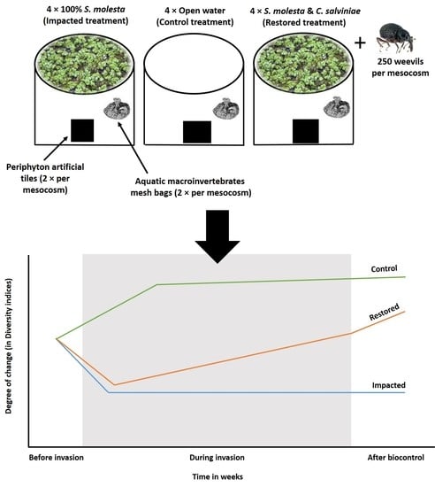
2.2. Experimental Design

To quantify the impact of S. molesta and its subsequent biological control, in terms of epilithic algae and aquatic macroinvertebrate diversity and community assemblage structure, an extension to the standard BACI design was employed. Twelve non-transparent mesocosm pools (diameter = 260 cm, height = 68 cm, total volume = 3600 L), were set-up at the Life Sciences Building (−33°30.9′94.9″ E, 26°51.8′70.6″ S), Rhodes University, Grahamstown, South Africa. Each pool was filled with tap water to a total volume of 3000 L and allowed to acclimate under natural environmental conditions for 7 days. Thereafter, mesocosm units were divided into three treatments: 100% S. molesta (impacted); S. molesta and C. salviniae (restored); and open water (control) treatments, making up 12 sampling units (3 treatments × 4 replicates). The experiment was stationed within a 15 m radius from a small stream (with different physicochemical characteristics to the mesocosms) on the periphery of Rhodes University, which assisted aquatic macroinvertebrate recruitment. The experiment was allowed to run for 60 weeks with six-weekly sampling collection (defined below), starting from February 2018 to April 2019.

Epilithic algae and aquatic macroinvertebrate assemblage structure and biodiversity indices, together with water physicochemistry datasets between treatments and S. molesta invasion phases, were used as proxies to estimate ecosystem recovery. Data collection consisted of three sampling phases: (1) the “before” invasion phase (before S. molesta invasion), (2) the “during” invasion phase (during S. molesta invasion), and (3) the “after” biological control phase (after biological control of S. molesta) (Figure 1). During the “before” invasion phase, mesocosm were S. molesta-free and were left for a period of 6 weeks, and artificial substrates were used to estimate epilithic algae and aquatic macroinvertebrate recruitment. At the end of the 6-week recruitment period, physicochemistry, epilithic algae, and aquatic macroinvertebrate taxa abundance, diversity, and assemblage composition data were collected (see below for details).

Following the “before” invasion phase, weevil-free S. molesta plants (50 kg per mesocosm) maintained in culture at the Centre for Biological Control’s Waainek Mass Rearing Research Facility (CBC-WMRRF), Rhodes University, were introduced into the impacted (100% S. molesta) and restored (S. molesta and C. salviniae) treatment mesocosms, leaving the open water treatment as a control (Figure 1). The transplanted S. molesta plants were left to grow under the following nutrient regime: a once-off addition of Culterra Multisol ‘N’ fertiliser (5 mg/L) and commercial iron chelate (100 mg Fe/L; 13% Fe, Ethylenediaminetetraacetic (EDTA)-FeNa-3H₂O) followed by a continuous Multicote slow release crystal fertiliser (nitrogen/phosphate/potassium 15:7:15, Haifa manufactures) in a plastic diffuser unit to promote growth of healthy S. molesta plants. After 60 days, 100% S. molesta cover was achieved, and the plastic diffuser units were removed. A total of 1000 individual C. salviniae weevils collected from stock cultures maintained at the CBC-WMRRF were then introduced to the restored (S. molesta and C. salviniae) treatment mesocosms (250 C. salviniae weevils per mesocosm), initiating the “during” invasion phase, which ran for 42 weeks (7 × 6-weekly sampling occasions). Following biological control of S. molesta, defined as complete S. molesta biomass clearing using biological control to clear-water state, the “after” biological control phase began and ran for 12 weeks (Figure 1).

2.3. Data Collection

2.3.1. Water Physicochemical Variables

Physicochemical data were measured every 6 weeks in each mesocosm from the start of the study, and included pH, conductivity (EC, µS), total dissolved solids (TDS, ppm), salinity (ppm), and water temperature (°C), using a Eutech multi-parameter testr 35 Series. DO concentration (mg/L) and water clarity (cm) were measured using a DO Pen Sper-Scientific (850045) meter and a water clarity tube (manufactured by GroundTruth, Hilton, South Africa). Additionally, water samples (500 mL) from each mesocosm were collected and taken to the laboratory to determine nitrate (NO₃) and ammonium (NH₄) using ion-specific electrodes (Range: 1.0 to 100 mg/L; manufactured by Vernier LabQuest2, Beaverto, USA) and phosphate (P) concentrations using a HI 83203 Multiparameter Bench Photometer for Aquaculture (range: 0.0 to 30.0 mg/L). Salvinia molesta percentage cover for the restored and impacted treatments was estimated visually every 6 weeks throughout the study.

2.3.2. Biological Data

Epilithic Algae Assemblage

To quantify epilithic algae (e.g., aquatic microalgae found growing on hard natural (stones) and/or artificial (stone tiles) substrates) species and assemblage structure between treatments and invasion phases, two plates of artificial substrate (22 × 22 cm stone tiles) were deployed at the base of each mesocosm and allowed to stand for a period of 6 weeks to allow periphyton colonisation [38]. On each sampling occasion, both tiles were retrieved from the mesocosms, placed onto a white collecting tray with approximately 1000 mL of filtered mesocosm water added, and the periphyton biofilm was then completely brushed off using a new toothbrush [39]. The resulting 1000 mL periphyton sample was divided into two 500 mL sub-samples for epilithic algae community and periphyton algae biomass using chlorophyll-a (Chl-a) analysis (described below). The community analysis sub-samples were transferred into clear polyethylene 500 mL containers and immediately preserved with 5 mL of Lugol’s iodine solution (prepared by dissolving 100 g potassium iodide and 50 g iodine crystals in 2 L of distilled water). Samples were then taken to the laboratory and allowed to sediment on a flat stable bench surface for 72 h [40]. Thereafter, 450 mL of the sample supernatant was extracted using a top-down siphoning system, and care was taken not to agitate the sample during the process. A total of 50 mL of the remaining concentrated epilithic algae sample was homogenised by moderately agitating the sample contents by hand for 5 s to evenly distribute epilithic algae cells. A Pasteur pipette was used to remove about ≈0.1 mL of the sample, which was placed onto a haemocytometer counting chamber (Neubauer improved; 0.1 depth, with a total grid area of 9 mm²), and covered with a cover slip [41]. Epilithic algae cell identification to the lowest possible taxonomic level (commonly species) and counting was conducted using a combination of field guides and identification keys, including John et al. [41], Van Vuuren et al. [42], and Taylor et al. [43], under a light-phase microscope (Olympus CX21) at 400X magnification.

Cell counting was declared sufficient and to have satisfied statistical requirements (cell concentration with a precision of ±10%) when either a maximum of 400 epilithic algae cells or a total of four 9 mm² grid counting area was achieved (equivalent to 4 × 9 mm² = 36 mm² counting grid area) per sub-sample [44]. Thereafter, to estimate the relative abundance of epilithic algae cells/mL, a modified LeGresley and McDermott [40] equation was used, taking total sample volume, concentrated sample volume, the number of grids counted, and 0.1 constant (standard chamber depth) into account:

$$\mathrm{Cells}/\mathrm{mL}=\frac{Cells counted\times Concentrated sample volume}{number of grids counted\times 0.1}\times Total sample volume$$

Phytoplankton and Periphyton Algal Biomass

To determine the productivity of each mesocosm between treatments and invasion phases, phytoplankton and periphyton algae biomass was used to estimate ecosystem net productivity. Using opaque polyethylene sample containers, 500 mL water samples (phytoplankton algae samples) were collected from each mesocosm, and together with the periphyton algae biomass sub-samples (previously collected) were stored on ice until later laboratory analysis. The storage method limited light penetration and kept the samples at a lower temperature to inhibit photosynthesis and other cellular processes from taking place that might lead to algal biomass misinterpretation. Prior to algae biomass determination, samples were homogenised by moderately agitating by hand for 5 s; thereafter, a standard sample volume of 200 mL phytoplankton and 100 mL periphyton samples were filtered through Millipore nylon net filters (50 mm diameter, 20 µm mesh size) using a vacuum pump (Instruvac Rocker 300) at 20 kPa. After filtering, any small unwanted animals (e.g., zooplankton and small invertebrates) and plant matter (e.g., Wolffia, Lemna species and debris) were removed from the nylon filter nets using forceps.

The acetone extraction method was used to determine phytoplankton and periphyton algal biomass fluorometrically, following Holm-Hansen and Riemann [45]. Briefly, each filtered nylon net was folded in half and placed into a 20 mL reaction tube with a screw, and then 10 mL of 90% acetone solution was added. The reaction tubes were left in complete darkness at −20 °C for a minimum of 48 h for Chl-a extraction. Thereafter, the Chl-a wavelength reading was determined using a 10AU Field and laboratory fluorometer (Tuner Designs), noting the wavelength reading before and after the sample was acidified by adding 2/3 drops of 0.1 M hydrochloric acid [46]. The final algae biomass was then calculated using the following formula modified from Lorenzen [47] and Daemen [48]:

$$\mathrm{Chl}\text{-}\mathrm{a} (\mathrm{mg}/{\mathrm{m}}^3) = \left(\frac{Acetone volume}{Filtered sample volume}\right)\times \left(Reading before acidificantion-Reading after acidification\right)\times 0.325$$

Aquatic Macroinvertebrates

Aquatic macroinvertebrate family-level identification is considered an efficient, easy-to-use, and reliable rapid assessment method for monitoring aquatic ecosystem impacts [49]. To estimate aquatic macroinvertebrate diversity and community assemblage structure between treatments and invasion phases, two types of artificial substrates, namely, 30 g plastic strips and 60 g plant matter (a combination of leaves, twigs, and stems), were used to sample colonisation by aquatic macroinvertebrates [50]. Artificial substrates were put in mesh bags (1 cm width mesh size) and then suspended mid-depth with string and placed on opposite sides of each mesocosm for a period of 6 weeks, which is a standard period to allow aquatic macroinvertebrate colonisation in standing water bodies [51]. After 6 weeks, the artificial substrates were retrieved from each mesocosm using a hand-held aquatic net (30 × 30 cm square frame, 1 mm mesh size) to prevent aquatic macroinvertebrates from escaping during collection. The mesh bag with artificial substrates were placed into a white sorting tray, and the contents of each mesh bag were emptied and rinsed with water in order to wash off and dislodge all aquatic macroinvertebrate samples into the tray. Samples were then left to settle for 2 min, and then identified to family-level for insects and class/sub-class for non-insects using multiple identification guides [52,53,54,55,56].

2.4. Data Analysis

2.4.1. Physicochemical Variables

A two-way analysis of variance (ANOVA) investigated the effect of treatment, invasion phases, and their interaction on the physicochemical variables (e.g., pH, EC, TDS, salinity, water temperature, [DO], [NO₃], [NH₄], [P], phytoplankton algae biomass, periphyton algae biomass, and water clarity). Because the physicochemical variables were not normally distributed (Shapiro–Wilk; p < 0.001, in all cases) and the variances were not homogeneous (Levene’s test, p > 0.05, in all cases), the data were log(x + 1) transformed to improve heteroscedasticity. All statistical analyses, except when specified, were conducted in R version 3.6.1 [57].

2.4.2. Epilithic Algae and Aquatic Macroinvertebrate Diversity Patterns and Response Ratios

To estimate epilithic algae and aquatic macroinvertebrate biodiversity indices between treatments and invasion phases, relative taxa abundance (N), taxa richness (S), Shannon–Weaver diversity (H’), and Pielou’s evenness (J’) were computed in R using the “vegan” package [58].

Then, to estimate the recovery of epilithic algae and aquatic macroinvertebrate biodiversity indices following biological control of S. molesta by C. salviniae, we calculated mean response ratios for each diversity indices [59,60]. The mean response ratios [59], for impacted treatment (100% S. molesta) =$\ln \left(\frac{Restored}{Impacted}\right)$ and control treatment (open water) =$\ln \left(\frac{Restored}{Control}\right)$ were compared to the restored treatment (S. molesta and C. salviniae) to estimate the effect size (e.g., change in biodiversity indices) following biological control by C. salviniae. Thereafter, a Wilcoxon signed rank test (wilcox.test function; p < 0.05) determined whether the mean response ratios were different from zero to ascertain whether the application of biological control affected epilithic algae and aquatic macroinvertebrate biodiversity indices. Thereafter, a Kruskal–Wallis ANOVA (kruskal.test function; p < 0.05) tested for significant differences in mean response ratios between treatments.

An extension of the BACI analysis (before–during–after invasion x control–impacted–restored) experimental design was employed to investigate the effect of epilithic algae and aquatic macroinvertebrate biodiversity indices on treatments and invasion phases. Prior to analysis, epilithic algae relative taxa abundance, taxa richness, and Shannon–Weaver diversity data were ln(x + 1) transformed to meet normality-distributed residuals and homoscedasticity. A linear mixed-effects model and a Tukey post-hoc test using “lme4” and “multcomp” packages were used to test the main effects and the interactions [61], respectively, where fixed effects were treatments (control, impacted, and restored) and invasion phases (before, during, and after invasion), and mesocosms were treated as random effects. Kenward–Roger approximations of degrees of freedom were used to obtain estimated F and p-values [62]. The variance explained by each model is reported as marginal R², which describes the proportion of variance explained by the fixed factor(s) alone, and conditional R², which describes the proportion of variance explained by both the fixed and random factors using the r.squaredGLMM function from the “MuMIn” package [63]. Model predictions were compared between treatments and invasion phases using Tukey’s HSD (honestly significant difference) (α = 0.05); however, they were adjusted to account for multiple comparisons using Holm’s sequential Bonferroni correction [64]. The model fit was inspected using residuals and fitted values plots and were found to satisfy the assumptions of normality and heterogeneity [65].

2.4.3. Epilithic Algae and Aquatic Macroinvertebrate Community Assemblage Structure

To investigate epilithic algae and aquatic macroinvertebrate assemblage structure between treatments and shifts between invasion phases, a permutational analysis of multivariate dispersions (PERMDISP; 9999 permutations) based on the mean distance to the centroid was performed on all epilithic algae and aquatic macroinvertebrate-relative taxa abundance to test for homogeneity of variances [66]. Additionally, a permutational multivariate analysis of variance (PERMANOVA) was tested, as well as whether epilithic algae and aquatic macroinvertebrate assemblages were different between treatments and invasion phases. A number of unconstrained ordinations were completed using principal coordinate analysis ordination (PCO) on Bray–Curtis similarity matrices to visualise both epilithic algae and aquatic macroinvertebrate assemblage structure. The PCO ordination was followed by a constrained canonical analysis of principal coordinates (CAP) ordination to emphasise and visualise epilithic algae and aquatic macroinvertebrate community assemblage patterns between treatments and invasion phases. Epilithic algae and aquatic macroinvertebrate relative taxa abundances were fourth-root transformed and correlated using the Pearson’s correlation (r > 0.5) with the canonical axes of the CAP to identify taxa driving the differences in assemblage structure between treatments and invasion phases [67]. Analyses were performed using PRIMER version 6 with the PERMANOVA add-on [68,69].

2.4.4. Biological Diversity Responses to Physicochemical Variables

Multiple linear regression analysis using the lm function in the “MASS” package was used to examine which physicochemical variables influenced epilithic algae and aquatic macroinvertebrate biodiversity indices. The initial model included the following variables: pH, EC, TDS, salinity, water temperature, [DO], [NO₃], [NH₄], [P], water clarity, and S. molesta percentage cover. Prior to analysis, multi-collinear variables including TDS and salinity were removed on the basis of the variance inflation factor and ecological rationale, and thereafter the remaining physicochemical variables were log(x + 1) transformed. In addition, phytoplankton, periphyton algal biomass, and aquatic macroinvertebrate functional feeding guild percentage abundances, including collector-filters, collector-gatherers, grazers, shredders, and predators, assigned following Cummins and Klug [70], Palmer et al. [71], Ingram et al. [72], and Walker et al. [73], were included as potential explanatory variables to account for variability in aquatic macroinvertebrate and epilithic algae biodiversity indices. The StepAIC function from the package “MASS” [74] performed forward–backward selection of the predictor variables, and the best model, that is, the one with the lowest Akaike’s information criterion (AIC) score, was selected.

3. Results

3.1. Physicochemical Variables

Dissolved oxygen concentration, water clarity, and periphyton biomass were significantly different between treatments, invasion phases, and treatment × invasion phase (

Table 1. Summary of two-way ANOVA representing statistics of all physicochemical variables collected during the before–after control–impact study. Significant differences (p < 0.05) are highlighted in bold. Mean and standard deviation physicochemical variable per treatment and invasion phase are presented in Table S1. df—degrees of freedom.

Physicochemical Variables	Treatments (df = 2, 111)		Invasion Phases (df = 2, 111)		Treatment × Phase (df = 4, 111)
	F-Value	p-Value	F-Value	p-Value	F-Value	p-Value
pH	2.36	0.099	6.46	<0.01	6.14	<0.001
Conductivity (µS)	1.88	0.158	1.23	0.296	0.253	0.907
Total Dissolved Solids (ppm)	0.87	0.423	1.36	0.262	0.12	0.979
Salinity (ppm)	2.67	0.074	0.81	0.499	0.16	0.957
Dissolved Oxygen (mg/L)	21.74	<0.001	10.39	<0.001	3.15	0.017
Water temperature (°C)	2.44	0.092	31.27	<0.001	0.06	0.993
Water Clarity (cm)	27.034	<0.001	3.05	0.05	4.88	0.001
NO3 (mg/L)	20.23	<0.001	2.06	0.133	2.19	0.074
NH4 (mg/L)	3.49	0.03	0.97	0.383	0.32	0.863
P (mg/L)	9.12	<0.001	1.32	0.271	1.05	0.383
Phytoplankton biomass (mg/m3)	6.03	0.003	5.49	0.005	1.61	0.178
Periphyton biomass (mg/m3)	36.52	<0.001	11.45	<0.001	12.27	<0.001

), whereas pH was significantly different between invasion phases and treatment × invasion phase, water temperature only between invasion phases, and phytoplankton biomass between treatments and invasion phases (Table 1). Water nutrient concentrations (NO₃, NH₄, and P) were only significantly different between treatments (Table 1).

Water clarity and periphyton biomass were correlated, where high water clarity and high periphyton biomass were recorded in the control treatment during the “after” biological control phase. Low water clarity and low periphyton biomass were recorded in the impacted treatment also during the “after” biological control phase (Table S1). This shows that light penetration (water clarity) had a positive effect to periphyton biomass. On the contrary, water clarity and phytoplankton biomass were indirectly correlated, with the second highest water clarity and low phytoplankton biomass being recorded in the impacted treatment during the “before” invasion phase and the lowest water clarity and the highest phytoplankton biomass being recorded in the impacted treatment during the “after” biological control phase (Table S1). This indicates that high light penetration had a negative effect on phytoplankton biomass, whereas S. molesta cover had a positive effect on phytoplankton biomass.

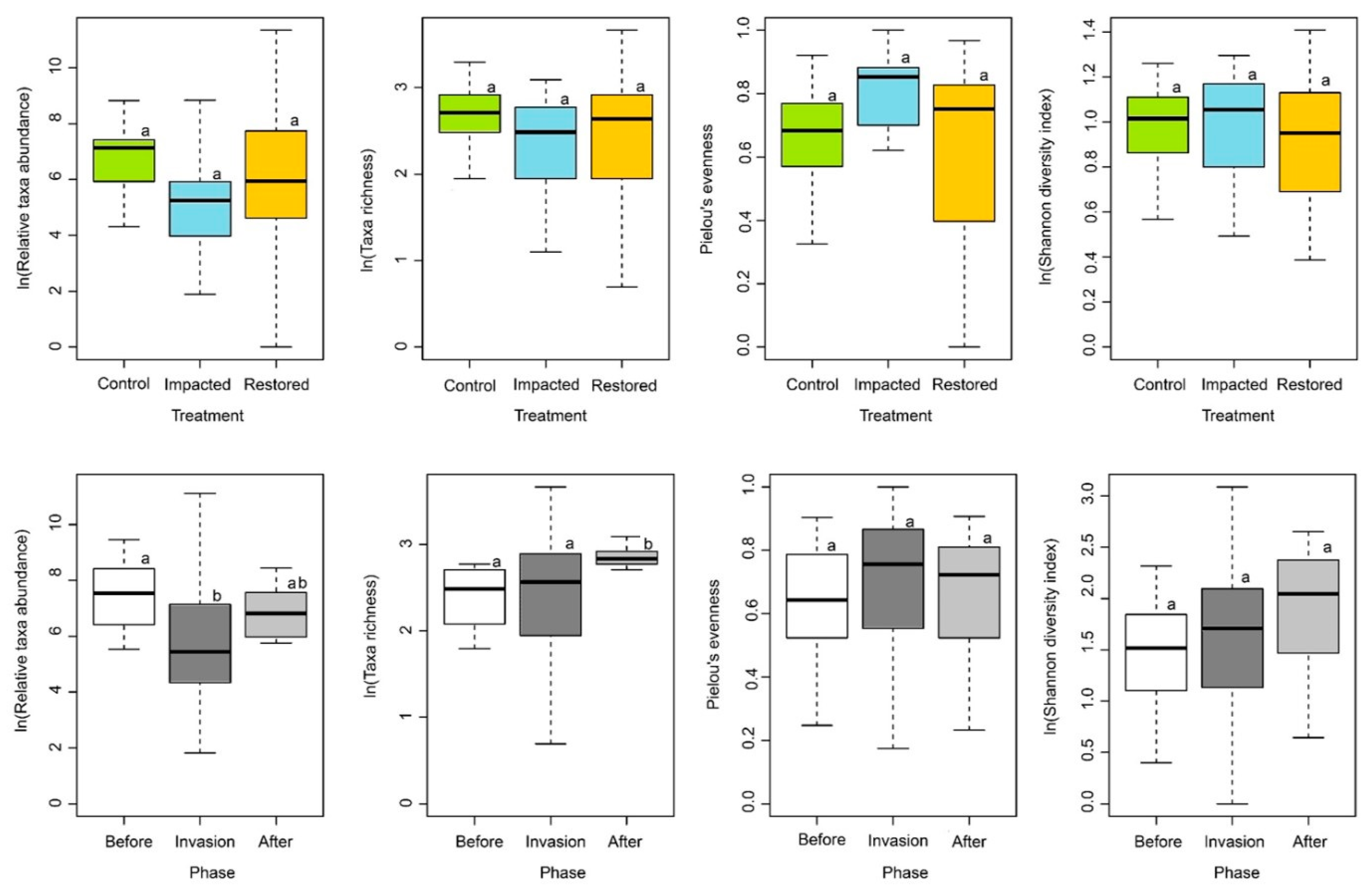
3.2. Epilithic Algae and Aquatic Macroinvertebrate Diversity Patterns

Linear mixed-effects models showed that the effect of treatment and treatment × invasion phase were not significantly different for epilithic algae biodiversity indices throughout the study. However, epilithic algae relative taxa abundance and taxa richness were significantly different between invasion phases (

Table 2. Summary of ANOVA type III for responses fitted with linear mixed-effects models. F values are represented with p-values on the basis of Kenward–Roger approximations for df (degrees of freedom). Significant differences (p < 0.05) are highlighted in bold. N = relative taxa abundance; S = taxa richness; J = Pielou’s evenness; H = Shannon–Weaver diversity index. Variance explained by each model is given by marginal R² for the fixed effects only and conditional R² for fixed and random effects.

Fixed Effects	N		S		J		H
	F	p	F	p	F	p	F	p
Epilithic algae
Treatment	0.59	0.56	0.57	0.57	1.32	0.29	0.33	0.72
Invasion phase	7.01	<0.01	2.90	0.05	0.08	0.91	1.01	0.37
Treatment × Invasion phase	1.07	0.38	1.12	0.35	1.13	0.35	1.65	0.17
R2marginal	0.21	-	0.15	-	0.07	-	0.21	-
R2conditional	0.23	-	0.15	-	0.18	-	0.23	-
Aquatic macroinvertebrates
Treatment	4.78	<0.05	24.24	<0.001	3.42	<0.05	22.11	<0.001
Invasion phase	4.14	<0.05	5.92	<0.01	5.48	<0.01	7.02	0.001
Treatment × Invasion phase	7.62	<0.001	8.44	<0.001	2.98	<0.05	4.47	<0.01
R2marginal	0.39	-	0.63	-	0.17	-	0.55	-
R2conditional	0.46	-	0.63	-	0.17	-	0.56	-

). In contrast, aquatic macroinvertebrate relative taxa abundance, taxa richness, Pielou’s evenness, and the Shannon–Weaver diversity were significantly different between treatments, invasion phases, and treatment × invasion phase (Table 2).

Relative epilithic algae abundance was highest during the “before” invasion phase, followed by the “after” biological control phase, and was the smallest in the “during” invasion phase (Figure 2, Figure S1). Comparatively, taxa richness was highest in the “after” biological control phase, when compared to the “before” and “during” invasion phases (Figure 2, Figure S1). Relative taxa abundances, taxa richness, Pielou’s evenness, and Shannon–Weaver diversity were not significantly different between treatments, however the control treatment showed high abundance and taxa richness, with the impacted treatment showing the least. Evenness and diversity was high in the impacted treatment in both cases, and the least in the control and restored treatments (Figure 2, Figure S1).

Aquatic macroinvertebrate relative taxa abundance and taxa richness were higher “after” biological control phase when compared to the “before” invasion phase, indicating relative recovery (Figure 3, Figure S2). The Shannon–Weaver diversity was higher in the “before” invasion phase, followed by the “after” biological control phase, with the “during” invasion phase recording the lowest diversity (Figure 3, Figure S2). Pielou’s evenness was highest “before” invasion and the lowest in the “after” biological control phase. Between treatments aquatic macroinvertebrate biodiversity indices were significantly different between invasion phases throughout the study (Figure 3, Figure S2). In all cases, the control treatment recorded the highest diversity scores, followed by the restored treatment, and the impacted treatment was the least diverse, except for Pielou’s evenness, which showed relatively equal means between the restored and impacted treatments (Figure 3, Figure S2).

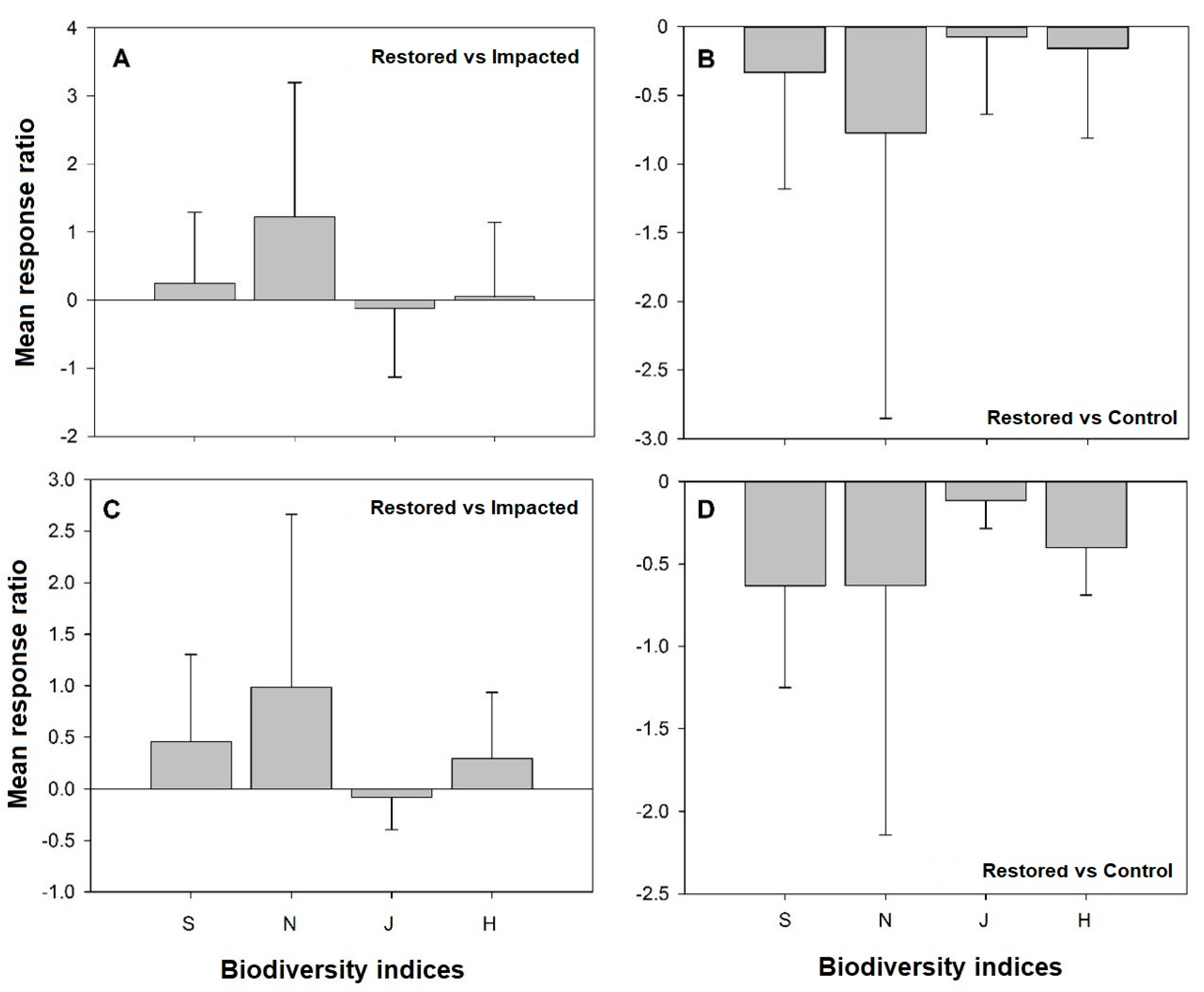
3.3. Biodiversity Indices Mean Response Ratios

Epilithic algae relative taxa abundance (W = 228, p < 0.001), taxa richness (W = 284.5, p < 0.01), and Pielou’s evenness (W = 494, p = 0.05) mean response ratios were significantly different from zero, unlike the Shannon–Weaver diversity (W = 358, p > 0.05) which was not different from zero (Figure 4A). Similarly, aquatic macroinvertebrate relative taxa abundance (W = 275, p < 0.001), taxa richness (W = 224, p < 0.001), and the Shannon–Weaver diversity (W = 186, p < 0.001) mean response ratios were significantly different from zero, but the opposite was true for Pielou’s evenness (W = 500, p > 0.05) (Figure 4C). This indicates that the S. molesta invasion and biological control by C. salviniae had an effect on epilithic algae and aquatic macroinvertebrate biodiversity indices.

Epilithic algae and aquatic macroinvertebrate relative taxa abundance, taxa richness, and the Shannon–Weaver diversity mean response ratios were greater than 0, and were less than 0 for Pielou’s evenness when the mean response ratio for the restored treatment was compared to the impacted treatment (Figure 4A,C), indicating a positive recovery following S. molesta biological control. Contrarily, the biodiversity indices’ mean response ratios between the restored and control treatments were less than zero in all cases, indicating that recovered biodiversity indices from restored treatment did not surpass that of the control treatment.

Epilithic algae relative taxa abundance (H = 12.64, p < 0.05), taxa richness (H = 7.62, p < 0.05), and Pielou’s evenness (H = 3.89, p = 0.05) were significantly different between the restored and control treatments (Figure 4A,B). Aquatic macroinvertebrate relative taxa abundance (H = 17.65, p < 0.05), taxa richness (H = 22.77, p < 0.05), and the Shannon–Weaver diversity (H = 25.10, p < 0.05) were also different between the restored and control treatments (Figure 4C,D). Overall, relative taxa abundance for both epilithic algae and aquatic macroinvertebrate recovered more effectively following the biological control of S. molesta by the weevil C. salviniae, followed by taxa richness and Shannon–Weaver diversity (Figure 4A,C).

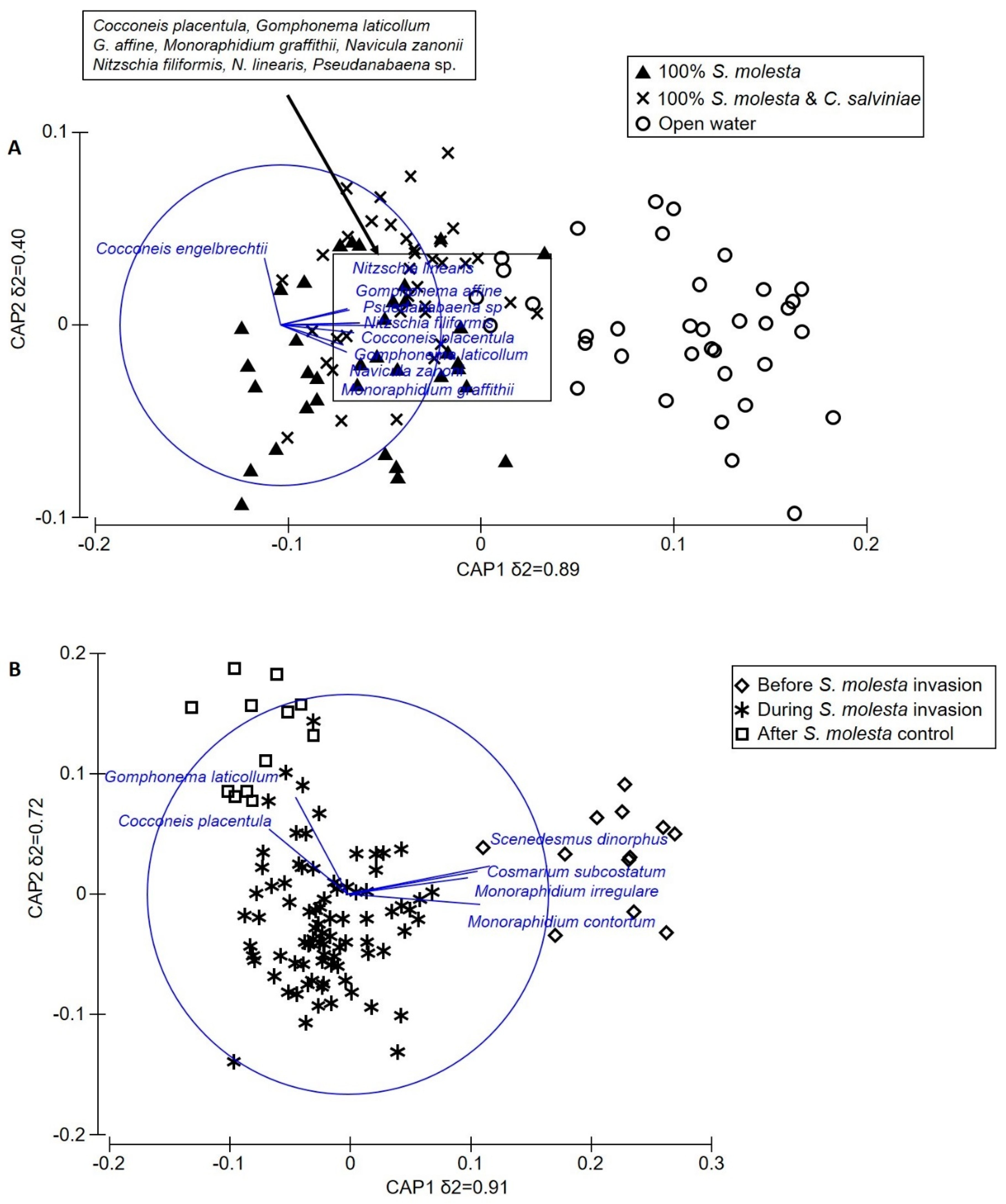
3.4. Epilithic Algae and Aquatic Macroinvertebrate Assemblage Structure

PERMANOVA reported significant differences in assemblage structure between treatments (epilithic algae, pseudo-F_{2, 111} = 2.77, p = 0.0001; aquatic macroinvertebrates, pseudo-F_{2, 111} = 6.61, p = 0.0001), invasion phases (epilithic algae, pseudo-F_{2, 111} = 5.56, p = 0.0001; aquatic macroinvertebrates, pseudo-F_{2, 111} = 13.91, p = 0.0001), and the interaction between treatment × invasion phase (epilithic algae, pseudo-F_{4, 111} = 1.56, p = 0.0004; aquatic macroinvertebrates, pseudo-F_{4, 111} = 3.50, p = 0.0001). Additionally, variances were heterogeneous in all cases for epilithic algae (PERMDISP, p < 0.05) and aquatic macroinvertebrates (PERMDISP, p < 0.05), and according to Anderson et al. [70], PERMANOVA is not affected by heterogeneity in variances.

Epilithic algae (Figure 5A,B) and aquatic macroinvertebrate (Figure 6A,B) assemblage structure were visually illustrated by CAP ordination. Epilithic algae assemblage composition between treatments and invasion phases showed three distinct clusters, where each cluster represented treatment (control, impacted, and restored) and invasion phase (before, during, and after invasion). The impacted and restored treatments explained 40% (δ² = 0.40) of the total variation in epilithic algae assemblage, indicating a degree of similarity (or overlap) (Figure 5A). Collectively, the impacted and restored treatments vs. control treatment explained a total variation of 89% (δ² = 0.89), indicating a completely different epilithic algae assemblage composition (Figure 5A). Cocconeis placentula, Gomphonema laticollum, Gomphonema affine, Nitzschia filiformis, Nitzschia linearis, Navicula zanonii, Monoraphidium graffithii, Pseudanabaena sp., and Cocconeis englebrechtii were strongly correlated with the control treatment (Pearson correlation, r > 0.5) (Figure 5A).

Similarly, epilithic algae assemblages were completely different between invasion phases, and this was supported by the high assemblage variation (or δ²) of 91% between “during” invasion and “before” invasion phases, and 72% between “during” invasion and “after” biological control phases (Figure 5B). Scenedesmus dinorphus, Cosmarium subcostatum, Monoraphidium irregular, and Monoraphidium contortum were strongly associated with the “before” invasion phase, compared to G. laticollum and C. placentula, which were associated with the “after” biological control phase (Figure 5B).

Aquatic macroinvertebrate assemblage structure responded to treatment and invasion phase, where each cluster represented a different treatment and invasion phase (Figure 6A,B). Canonical correlation for aquatic macroinvertebrate assemblages was δ² = 0.78 and δ² = 0.71 between treatments, and δ² = 0.80 and δ² = 0.67 between invasion phases for CAP axis 1 and 2, respectively, indicating complete separation/differences in aquatic macroinvertebrate assemblages between treatments and invasion phases. Hydrophilidae, Belostomatidae, and Hirudinea taxa showed a strong association (Pearson’s correlation, r > 0.5) to the restored and control treatments (Figure 6A). The “before” invasion phase was associated with Caenidae, Baetidae, and Notonectidae taxa, whereas the “after” biological control phase was favoured by both Hirudinea and Cypridoidae taxa (Figure 6B).

3.5. Biological Diversity Response to Physicochemical Variables

The functional feeding group collector-gatherers in aquatic macroinvertebrates, S. molesta cover, periphyton biomass, pH, water temperature, [DO], and [NH₄] as predictor variables explained 31% of epilithic algae relative taxa abundance variation. Salvinia molesta cover and pH were significant, and negatively affected relative epilithic algae abundance, whereas periphyton biomass positively affected relative epilithic algae abundance (

Table 3. Multiple linear regression analyses (summary lm R function) for epilithic algae biodiversity indices. The table shows estimates ± standard error (SE) t-statistics, adjusted R-squared values (AdjR²) and respective p-values for regression coefficients, indicating whether the value of the coefficient is significantly different from zero (α = 0.05). Significant differences are in bold. lnN, lnS, and lnH represent ln(x + 1) transformed biodiversity indices. Cover—Salvinia molesta percentage cover.

Diversity Indices	Predictors	Estimates	SE	t	p	AdjR2	df	F	p
Epilithic Algae
lnN	Intercept	31.047	7.008	4.430	<0.0001	0.308	7, 100	7.801	<0.0001
	Collector-gathers	0.260	0.140	1.852	0.067
	Cover	−0.543	0.095	−5.730	<0.0001
	pH	−10.114	3.311	−3.055	0.003
	Water temperature	−1.990	1.076	−1.850	0.067
	[DO]	1.354	0.896	1.512	0.134
	[NH4]	−9.915	6.857	−1.446	0.151
lnS	Intercept	9.789	2.102	4.658	<0.0001	0.209	5, 102	6.646	<0.0001
	Cover	−0.125	0.028	−4.549	<0.0001
	pH	−2.230	0.896	−2.490	0.014
	Water temperature	−0.724	0.312	−2.320	0.022
	[NH4]	−4.679	2.054	−2.278	0.248
	[P]	−0.151	0.106	−1.430	0.156
J	Intercept	0.642	0.034	18.677	<0.0001	0.027	2, 105	2.529	0.085
	Cover	0.016	0.011	1.511	0.133
	[NH4]	−1.511	0.878	−1.721	0.088
lnH	Intercept	4.806	2.086	2.304	0.023	0.044	3, 104	2.659	0.05
	pH	−1.404	0.959	−1.464	0.146
	[NH4]	−4.737	2.391	−1.981	0.050
	[P]	−0.206	0.123	−1.671	0.098

). Epilithic algae taxa richness was affected by S. molesta cover, pH, water temperature, [NH₄], and [P], explaining 21% variation in epilithic algae taxa richness. All variables negatively affected epilithic algae taxa richness, but only S. molesta cover, pH, and water temperature were significant (Table 3). The Shannon–Weaver diversity, on the other hand, was affected by pH, [NH₄], and [P], and explained 4.4% variation in of epilithic algae Shannon–Weaver diversity, where only [NH₄] showed a significant and negative correlation (Table 3).

Salvinia molesta cover, phytoplankton biomass, pH, and water temperature explained 44% and 41% variation in aquatic macroinvertebrate taxa richness and Shannon–Weaver diversity, respectively, during the study (

Table 4. Multiple linear regression analyses (summary lm R function) for aquatic macroinvertebrate biodiversity indices. The table shows estimates ± standard error (SE), t-statistics, adjusted R-squared values (AdjR²) and respective p-values for regression coefficients, indicating whether the value of the coefficient is significantly different from zero (α = 0.05). Significant differences are in bold. Cover—Salvinia molesta percentage cover.

Diversity Indices	Predictors	Estimates	SE	t	p	AdjR2	df	F	p
Aquatic Macroinvertebrates
N	Intercept	−7.341	3.608	−2.035	0.044	0.204	4, 115	8.617	<0.0001
	Cover	−0.122	0.046	−2.667	0.009
	Phytoplankton biomass	0.226	0.115	1.963	0.052
	pH	6.192	1.707	3.628	0.0004
	[DO]	−0.881	0.433	−2.032	0.045
S	Intercept	−39.085	13.11	−2.981	0.004	0.444	4, 115	24.74	<0.0001
	Cover	−1.030	0.157	−6.547	<0.0001
	Phytoplankton biomass	1.059	0.393	2.692	0.008
	pH	16.194	5.518	2.935	0.004
	Water temperature	4.957	1.745	2.841	0.005
J	Intercept	0.068	0.224	0.301	0.764	0.060	3, 116	3.52	0.017
	Water clarity	0.049	0.021	2.322	0.022
	Phytoplankton biomass	0.028	0.017	1.607	0.111
	Water temperature	0.153	0.070	2.190	0.031
H	Intercept	−3.902	1.547	−2.523	0.013	0.410	4, 115	21.64	<0.0001
	Cover	−0.111	0.019	−5.993	<0.0001
	Phytoplankton biomass	0.096	0.046	2.060	0.042
	pH	1.708	0.651	2.624	0.01
	Water temperature	0.629	0.209	3.102	0.002

). In both cases, S. molesta cover negatively correlated with aquatic macroinvertebrate taxa richness and Shannon–Weaver diversity, whereas phytoplankton biomass, pH, and water temperature positively influenced both taxa richness and the Shannon–Weaver diversity (Table 4). Salvinia molesta cover, phytoplankton biomass, pH, and [DO] explained 20% variation in aquatic macroinvertebrate relative taxa abundance, whereas only S. molesta cover and [DO] showed a negative correlation, in contrast to pH and phytoplankton biomass. Aquatic macroinvertebrate Pielou’s evenness was positively affected by water clarity, phytoplankton biomass, and water temperature, and collectively only explained 6% variation. Water clarity and water temperature were the only significant variables that showed a positive correlation with aquatic macroinvertebrate Pielou’s evenness (Table 4).

4. Discussion

This study showed that the presence of S. molesta negatively affected water quality (i.e., reduced DO concentration, light penetration, and water clarity) and aquatic biodiversity, which is consistent with the findings of Masifwa et al. [75], Brendonck et al. [76], Midgley et al. [77], Chamier et al. [78], and Coetzee et al. [27] for P. crassipes. Our findings supported our hypothesis, wherein the presence of free-floating IAAP species, such as S. molesta, alter aquatic biota assemblage structure, but that biological control improves water quality (e.g., increase in DO concentration, light penetration, and water clarity) and therefore results in aquatic biodiversity recovery. This study therefore justifies the biological control of IAAP species in novel environments to facilitate ecosystem recovery, as well as community structure re-organisation for normal ecosystem processes and functions.

Traditionally, terrestrial and aquatic biota community-based matrices have been used to assess or monitor environmental impacts. According to Adams et al. [79] and Muotka and Laasonen [80], species abundance, diversity, presence and absence of key species, and other community attributes are useful indicators of environmental change. Studies by Kettenring and Adams [81] and Prior et al. [82] reviewed alien invasive weed control methods that would translate to ecosystem recovery/restoration following alien invasive management, wherein both reviews reported mechanical control and excluded data from biological control methods, with the authors emphasising that there were no case-studies that included assessments of native flora and fauna regeneration following mechanical control, which is critical for rehabilitation. These authors recommended that the management of alien invasive species should be considered on a broader scale, including not only control, but also ecosystem recovery of invaded ecosystems. In the present study, epilithic algae and aquatic macroinvertebrate taxa richness, relative abundance, and Shannon–Weaver diversity responded negatively to S. molesta invasion, but positively following the biological control of S. molesta. Additionally, abiotic filters associated with S. molesta invasion had negative ecological impacts, which included reduced DO concentration and water clarity, as well as increased S. molesta cover, negatively affected measured biodiversity indices throughout the study. Relative taxa abundance, taxa richness, and Shannon–Weaver diversity also improved significantly following the biological control of S. molesta. These results demonstrate that the action of the biological control agent, C. salviniae, was sufficient in allowing ecosystem biodiversity recovery of the impacted mesocosm, where measured biodiversity indices were almost similar to that of the control conditions during the final “after” biological control phase.

The epilithic algae and aquatic macroinvertebrate assemblages were different between treatments and responded differently to different invasion phases. The control treatment was dominated by fast growing epilithic algae taxa including Nitzschia sp. and the low-light-sensitive species such as Scenedesmus sp. and Pseudanabaena sp., and comparatively the impacted and restored treatments were affected by light limitation and showed reduced ecosystem productivity and periphyton development and biomass. Similarly, during the “before” invasion phase, Scenedesmus dinorphus, Cosmarium subcostatum, and Monoraphidium contortum were the most dominant epilithic algae taxa, which are indicative of increase light penetration and low nutrients [72,73]. In both cases, the epilithic algae taxa abundance patterns were in agreement with the taxa ecologies and clearly responded to S. molesta invasion and associated water physicochemistry characteristics. The “before” invasion and the control treatments represented open water, which were characterised by sufficient light penetration, increased DO concentration, water clarity, and high periphyton development as compared to the “during” invasion and the impacted treatment; thus, S. molesta and associated abiotic filters were important factors influencing both biodiversity and assemblage structure in the present study. This was also the case for aquatic macroinvertebrate biodiversity and assemblage structure. In comparison with the control treatment, the restored treatment was dominated by Hydrophilidae and Belostomatidae, and both families are air-breathers, associated with a combination of vegetated and open water systems to display the shredder and predatory role [70]. The “before” invasion phase was dominated by Caenidae, Baetidae, and Notonectidae, known to be indicative of good water quality [49]. Following biological control, “after” biological control phase, generalist taxa and collector-feeders were more abundant, and this was attributed to available space and decaying S. molesta matter, which favoured both opportunistic and general filter feeders.

Abiotic filters (e.g., light limitation, reduced DO concentration, and reduced water clarity) introduced by S. molesta “during” invasion negatively affected both epilithic algae and aquatic macroinvertebrates, which was also seen in Midgley et al. [77]. Following the biological control of S. molesta and the alleviation of these abiotic filters in the restored treatment, we saw an increase in DO concentration, improved water clarity, periphyton biomass, and higher water temperatures, which supported increases in epilithic algae and aquatic macroinvertebrate abundances and biodiversity.

Benayas et al. [60] emphasise that biodiversity-ecosystem function studies have generally been laboratory based or have employed small field plots or mesocosms, as was the case in the present study. It might be argued that findings from such small-scale studies have little relevance to the ecosystem scale at which management decisions are made. However, such small-scale studies are building blocks that provide empirical evidence to help understand systems, so that when large-scale studies are conducted, fundamental ecological processes and feedback are better understood [83,84,85,86]. Benton et al. [87] further emphasise that microcosms and mesocosms are suitable experimental platforms to enable ecologists to test global ecological problems and provide empirical data that can be conceptualised to simplify some of the complex mechanisms that are necessary in ecological studies.

In conclusion, the present study provides useful empirical evidence of the impact of S. molesta on aquatic biodiversity, as well as how biological control facilitates biodiversity recovery when relevant biological indicators are employed. This study further proposes that successful biological control of IAAP species should be measured on the basis of the return of biological and functionally important aquatic biota, and not simply clearing of the target weed biomass and reducing plant demographics. Epilithic algae and aquatic macroinvertebrates were reliable biological indicators to measure the impact of S. molesta on ecosystems. We also support the use of community-based indices (e.g., relative abundances, taxa richness, and biodiversity), as they are sufficiently sensitive to detect environmental change and provide a rapid assessment tools. We recommend that similar studies should be replicated in the field and investigate the interactions of multiple trophic levels to better understand ecological feedback mechanisms under invasion and to understand if active restoration can be useful in repairing previously invaded ecosystems.

References

1. Bakker, E.S.; Sarneel, J.M.; Gulati, R.D.; Liu, Z.; van Donk, E. Restoring macrophyte diversity in shallow temperate lakes: Biotic versus abiotic constraints. Hydrobiologia 2013, 710, 23–37. [Google Scholar] [CrossRef] [Green Version]
2. Hill, M.P. The impact and control of alien aquatic vegetation in South African aquatic ecosystems. Afr. J. Aquat. Sci. 2003, 28, 19–24. [Google Scholar] [CrossRef]
3. Hill, M.P.; Coetzee, J. The biological control of aquatic weeds in South Africa: Current status and future challenges. Bothalia 2017, 47, 1–12. [Google Scholar] [CrossRef]
4. De Tezanos Pinto, P.; Allende, L.; O’Farrell, I. Influence of free-floating plants on the structure of a natural phytoplankton assemblage: An experimental approach. J. Plankton Res. 2007, 29, 47–56. [Google Scholar] [CrossRef] [Green Version]
5. Callaway, R.M.; Aschehoug, E.T. Invasive plants versus their new and old neighbors: A mechanism for exotic invasion. Science 2002, 290, 521–523. [Google Scholar] [CrossRef]
6. Corbin, J.D.; D’Antonio, C.M. Abundance and productivity mediate invader effects on nitrogen dynamics in a California grassland. Ecosphere 2011, 2. [Google Scholar] [CrossRef]
7. Van Wilgen, B.W.; Raghu, S.; Sheppard, A.W.; Schaffner, U. Quantifying the social and economic benefits of the biological control of invasive alien plants in natural ecosystems. Curr. Opin. Insect Sci. 2020, 38, 1–5. [Google Scholar] [CrossRef]
8. Mcfadyen, R.E.C. Successes in biological control of weeds. Proc. X Int. Symp. Biol. Control Weeds 2000, 14, 3–14. [Google Scholar]
9. Van Driesche, R.G.; Pratt, P.D.; Huber, J.; Hough-Goldstein, J.; Newman, R.; Sands, D.; Causton, C.E.; Cuda, J.; Miller, R.; Ding, J.; et al. Classical biological control for the protection of natural ecosystems. Biol. Control 2010, 54, S2–S33. [Google Scholar] [CrossRef]
10. McConnachie, A.J.; De Wit, M.P.; Hill, M.P.; Byrne, M.J. Economic evaluation of the successful biological control of Azolla filiculoides in South Africa. Biol. Control 2003, 28, 25–32. [Google Scholar] [CrossRef]
11. Fraser, G.C.G.; Hill, M.P.; Martin, J.A. Economic evaluation of water loss saving due to the biological control of water hyacinth at New Year’s Dam, Eastern Cape province, South Africa. Afr. J. Aquat. Sci. 2016, 41, 227–234. [Google Scholar] [CrossRef]
12. Arp, R.; Fraser, G.; Hill, M. Quantifying the water savings benefit of water hyacinth (Eichhornia crassipes) control in the Vaalharts Irrigation Scheme. Water SA 2017, 43, 58–66. [Google Scholar] [CrossRef] [Green Version]
13. Coetzee, A.J.A.; Hill, M.P.; Byrne, M.J.; Bownes, A. A review of the biological control programmes on Eichhornia crassipes (C. Mart) Solms (Pontederiaceae), Salvinia molesta D. S. Mitch. (Salviniaceae), Pistia stratiotes L. (Araceae), Myriophyllum aquaticum (Vell.) Verdc. (Haloragaceae) and Azolla filiculoides Lam. (Azollaceae) in South Africa. Afr. Entomol. 2011, 19, 451–468. [Google Scholar]
14. Cuda, J.P.; Charudattan, R.; Grodowitz, M.J.; Newman, R.M.; Shearer, J.F.; Tamayo, M.L.; Villegas, B. Recent advances in biological control of submersed aquatic weeds. J. Aquat. Plant Manag. 2008, 46, 15–32. [Google Scholar]
15. Maseko, Z.; Coetzee, J.A.; Hill, M.P. Effect of shade and eutrophication on the biological control of Salvinia molesta (Salviniaceae) by the weevil Cyrtobagous salviniae (Coleoptera: Erirhinidae). Austral Entomol. 2019, 58, 595–601. [Google Scholar] [CrossRef]
16. Martin, G.D.; Coetzee, J.A.; Weyl, P.S.R.; Parkinson, M.C.; Hill, M.P. Biological control of Salvinia molesta in South Africa revisited. Biol. Control 2018, 125, 74–80. [Google Scholar] [CrossRef]
17. Schaffner, U.; Hill, M.; Dudley, T.; D’Antonio, C. Post-release monitoring in classical biological control of weeds: Assessing impact and testing pre-release hypotheses. Curr. Opin. Insect Sci. 2020, 38, 99–106. [Google Scholar] [CrossRef]
18. Hulme, P.E. Beyond control: Wider implications for the management of biological invasions. J. Appl. Ecol. 2006, 43, 835–847. [Google Scholar] [CrossRef]
19. Underwood, A.J. Beyond BACI: The detection of environmental impacts on populations in the real, but variable, world. J. Exp. Mar. Bio. Ecol. 1992, 161, 145–178. [Google Scholar] [CrossRef]
20. Pryke, J.S.; Samways, M.J. Recovery of invertebrate diversity in a rehabilitated city landscape mosaic in the heart of a biodiversity hotspot. Landsc. Urban Plan. 2009, 93, 54–62. [Google Scholar] [CrossRef]
21. Magoba, R.N.; Samways, M.J. Recovery of benthic macroinvertebrate and adult dragonfly assemblages in response to large scale removal of riparian invasive alien trees. J. Insect Conserv. 2010, 14, 627–636. [Google Scholar] [CrossRef]
22. Samways, M.J.; Sharratt, N.J.; Simaika, J.P. Effect of alien riparian vegetation and its removal on a highly endemic river macroinvertebrate community. Biol. Invasions 2011, 13, 1305–1324. [Google Scholar] [CrossRef]
23. Modiba, R.V.; Joseph, G.S.; Seymour, C.L.; Fouché, P.; Foord, S.H. Restoration of riparian systems through clearing of invasive plant species improves functional diversity of Odonate assemblages. Biol. Conserv. 2017, 214, 46–54. [Google Scholar] [CrossRef]
24. Covich, A.P.; Palmer, M.A.; Crowl, T.A. The role of benthic invertebrate species in freshwater ecosystems: Zoobenthic species influence energy flows and nutrient cycling. Bioscience 1999, 49, 119–127. [Google Scholar] [CrossRef] [Green Version]
25. Kietzka, G.J.; Pryke, J.S.; Samways, M.J. Landscape ecological networks are successful in supporting a diverse dragonfly assemblage. Insect Conserv. Diver. 2015, 8, 229–237. [Google Scholar] [CrossRef]
26. Liboriussen, L.; Jeppesen, E. Structure, biomass, production and depth distribution of periphyton on artificial substratum in shallow lakes with contrasting nutrient concentrations. Freshw. Biol. 2006, 51, 95–109. [Google Scholar] [CrossRef]
27. Coetzee, J.A.; Jones, R.W.; Hill, M.P. Water hyacinth, Eichhornia crassipes (Pontederiaceae), reduces benthic macroinvertebrate diversity in a protected subtropical lake in South Africa. Biodivers. Conserv. 2014, 23, 1319–1330. [Google Scholar] [CrossRef]
28. Stiers, I.; Crohain, N.; Josens, G.; Triest, L. Impact of three aquatic invasive species on native plants and macroinvertebrates in temperate ponds. Biol. Invasions 2011, 13, 2715–2726. [Google Scholar] [CrossRef]
29. Thomas, P.; Room, P. Towards biological control of salvinia in Papua New Guines. Proc. Int. Symp. Biol. Control Weeds 1985, 567–574. [Google Scholar]
30. Nelson, L.S.; Skogerboe, J.G.; Getsinger, K.D. Herbicide evaluation against giant salvinia. J. Aquat. Plant Manag. 2001, 39, 48–53. [Google Scholar]
31. Julien, M.H.; Hill, M.P.; Tipping, P.W. Salvinia molesta D. S. Mitchell (Salviniaceae). In Biological Control of Tropical Weeds Using Arthropods; Muniappan, R., Reddy, G.V.P., Raman, A., Eds.; Cambridge University Press: Cambridge, UK, 2009; pp. 378–407. ISBN 9780511576348. [Google Scholar]
32. Hennecke, B.; Postle, L. The key to success: An investigation into oviposition of the salvinia weevil in cool climate regions. In Proceedings of the 15th Australia Weeds Conference, Weed Management Society of South Australia, Adelaide, South Australia, 24–28 September 2006; pp. 780–783. [Google Scholar]
33. Room, P.M.; Thomas, P.A. Nitrogen, phosphorus and potassium in Salvinia molesta Mitchell in the field: Effects of weather, insect damage, fertilizers and age. Aquat. Bot. 1986, 24, 213–232. [Google Scholar] [CrossRef]
34. Flores, D.; Wendel, L. Proposed Field Release of the Salvinia Weevil, Cyrtobagous Salviniae Calder and Sands (Curculionidae: Coleoptera), A Host-Specific Biological Control Agent of Giant Salvinia, Salvinia Molesta D.S. Mitchell (Salviniaceae: Polypodiophyta) A Federal Noxious Weed; USD/APHIS/PPQ/CPHST/Mission Plant Protection Center (MPPC): Edinburg, TX, USA, 2001. [Google Scholar]
35. Oliver, J.D. A review of the biology of giant salvinia (Salvinia molesta Mitchell). J. Aquat. Plant Manag. 1993, 31, 227–231. [Google Scholar]
36. Doeleman, J.A. Biological Control of Salvinia Molesta in Sri Lanka: An Assessment of Costs and Benefits; No 1–No 12; Australian Center for International Agricultural Research: Canberra, Australia, 1989; p. 14. ISBN 1949511978. [Google Scholar]
37. Sullivan, P.; Postle, L. Salvinia Biological Control Field Guide; Department of Trade and Investment, Regional Infrastructure and Services: Sydney, Australia, 2012; ISBN 9781742562520. [Google Scholar]
38. Kelly, M.G.; Cazaubon, A.; Coring, E.; Dell’Uomo, A.; Ector, L.; Goldsmith, B.; Guasch, H.; Hurlimann, J.; Jarlman, A.; Kawecka, B.; et al. Recommendations for the routine sampling of diatoms for water quality assessments in Europe. J. Appl. Phycol. 1998, 10, 215–224. [Google Scholar] [CrossRef]
39. Taylor, J.C.; Harding, W.R.; Archibald, C.G.M. A Methods Manual for the Collection, Preparation and Analysis of Diatom Samples Version 1.0; Water Research Commission: Pretoria, South Africa, 2007; pp. 1–49. [Google Scholar]
40. LeGresley, M.; McDermott, G. Counting chamber methods for quantitative phytoplankton analysis-haemocytometer, Palmer-Maloney cell and Sedgewick-Rafter cell. In Manuals and Guides: Microscopic and Molecular Methods for Quantitative Phytoplankton Analysis, 55th ed.; Karlson, B., Cusack, C., Bresnan, E., Eds.; United Nations Educational, Scientific and Cultural Organisation: Paris, France, 2000; pp. 25–30. [Google Scholar]
41. John, D.; Whitton, B.; Brook, A.J. (Eds.) The Freshwater Algal Flora of the British Isles An Identification Guide to Freshwater and Terrestrial Algae; Cambridge University Press: Cambridge, UK, 2002. [Google Scholar]
42. Van Vuuren, J.; Taylor, J.; van Ginkel, C.; Gerber, A. A Guide for the Identification of Microscopic Algae in South African Freshwaters; North West University and Department of Water Affairs and Forestry: Pretoria, South Africa, 2006; ISBN 0621354716. [Google Scholar]
43. Taylor, J.C.; Harding, W.R.; Archibald, G.M. An Illustrated Guide to Some Common Diatom Species from South Africa; Water Research Commission: Pretoria, South Africa, 2007; ISBN 09263373. [Google Scholar]
44. Andersen, P.; Throndsen, J. Estimating cell numbers. In Monographs on Oceanographic Methodology: Manual on Harmful Marine Microalgae; Hallegraeff, G., Anderson, D., Cembella, A., Eds.; United Nations Educational, Scientific and Cultural Organisation: Paris, France, 2003; pp. 99–130. ISBN 9231039482. [Google Scholar]
45. Holm-hansen, O.; Riemann, B. Chlorophyll-a determination: Improvements in Methodology. Oikos 1978, 30, 438–447. [Google Scholar] [CrossRef]
46. Dalu, T.; Froneman, P.W.; Richoux, N.B.; Dalu, T.; Froneman, P.W. Phytoplankton community diversity along a river- estuary continuum. Trans. R. Soc. South Afr. 2014, 69, 107–116. [Google Scholar] [CrossRef]
47. Lorenzen, C. Determination for chlorophyll and pheophytin pigments. Plant Physiol. 1967, 12, 343–346. [Google Scholar]
48. Daemen, E.A.M.J. Comparison of methods for the determination of chlorophyll in estuarine sediments. Neth. J. Sea Res. 1986, 20, 21–28. [Google Scholar] [CrossRef]
49. Dickens, C.W.S.; Graham, P.M. The South African scoring system (SASS) version 5 rapid bioassessment method for rivers. Afr. J. Aquat. Sci. 2002, 27, 1–10. [Google Scholar] [CrossRef]
50. Booth, A.J.; Kadye, W.T.; Vu, T.; Wright, M. Rapid colonisation of artificial substrates by macroinvertebrates in a South African lentic environment. Afr. J. Aquat. Sci. 2013, 38, 175–183. [Google Scholar] [CrossRef]
51. Thirion, C. A new biomonitoring protocol to determine the ecological health of impoundments using artificial substrates. Afr. J. Aquat. Sci. 2000, 25, 123–133. [Google Scholar] [CrossRef]
52. Day, J.A.; de Moor, I.J. Guides to the Freshwater Invertebrates of Southern Africa. Volume 5: Non-Arthropods; Water Research Commission: Pretoria, South Africa, 2002. [Google Scholar]
53. Day, J.A.; de Moor, I.J.; Stewart, B.A.; Louw, A. Guides to the Freshwater Invertebrates of Southern Africa. Volume 3: Crustacea II; Water Research Commission: Pretoria, South Africa, 2001. [Google Scholar]
54. Day, J.A.; de Moor, I.J. Guides to the Freshwater Invertebrates of Southern Africa. Volume 6: Arachnida and Mollusca; Water Research Commission: Pretoria, South Africa, 2002. [Google Scholar]
55. Day, J.A.; Stewart, B.; de Moor, I.J.; Louw, A. Guides to the Freshwater Invertebrates of Southern Africa. Volume 4: Crustacea III; Water Research Commission: Pretoria, South Africa, 2001. [Google Scholar]
56. Gerber, A.; Gabriel, M. Aquatic Invertebrates of South African Rivers: Field Guide; Department of Water Affairs: Pretoria, South Africa, 2002. [Google Scholar]
57. Bunn, A.; Korpela, M. R Core Team R: A language and environment for statistical computing. R Found. Stat. Comput. 2016, 2, 2630. [Google Scholar]
58. Oksanen, J. Vegan: Ecological diversity. R Proj. 2013, 1, 12. [Google Scholar]
59. Hedges, L.V.; Gurevitch, J.; Curtis, P.S. The meta-analysis of response ratios in experimental ecology. Ecology 1999, 80, 1150–1156. [Google Scholar] [CrossRef]
60. Benayas, J.M.R.; Newton, A.C.; Diaz, A.; Bullock, J.M. Enhancement of biodiversity and ecosystem services by ecological restoration: A meta-analysis. Science 2009, 325, 1121–1124. [Google Scholar] [CrossRef]
61. Bates, D.; Machler, M.; Bolker, B.; Walker, S. Fitting linear mixed-effects models using lme4. J. Stat. Softw. 2015, 67, 1–48. [Google Scholar] [CrossRef]
62. Kenward, M.G.; Roger, J.H. An improved approximation to the precision of fixed effects from restricted maximum likelihood. Comput. Stat. Data Anal. 2009, 53, 2583–2595. [Google Scholar] [CrossRef]
63. Nakagawa, S.; Schielzeth, H. A general and simple method for obtaining R2 from generalized linear mixed-effects models. Methods Ecol. Evol. 2013, 4, 133–142. [Google Scholar] [CrossRef]
64. Holm, S. A simple sequentially rejective multiple test procedure. Scand. J. Stat. 1978, 6, 65–70. [Google Scholar]
65. Zuur, A.; Leno, E.; Walker, N.; Saveliev, A.; Smith, G. Mixed Effects Models and Extensions in Ecology with R; Springer: New York, NY, USA, 2006; ISBN 9780387874579. [Google Scholar]
66. Clarke, K.R.; Gorley, R.N. PRIMER v6: User manual/tutorial. PRIMER-E: Plymouth, UK, 2006; Available online: https://www.researchgate.net/profile/Saeed_Ebrahimnezhad_Darzi/post/looking_for_PDF_of_Primer_v6_User_Manual_Tutorial/attachment/59d6515879197b80779a9e3b/AS%3A506949617238016%401497877615728/download/ClarkeGorley+2006+PrimerV6UserManual.pdf (accessed on 1 December 2017).
67. Anderson, M.; Willis, T. Canonical analysis of principal coordinates: A useful method of constrained ordination for ecology. Ecology 2003, 84, 511–525. [Google Scholar] [CrossRef]
68. Clarke, K.R.; Gorley, R.N. PRIMER v6: User Manual and Tutorial; PRIMER-E: Plymouth, UK, 2006. [Google Scholar]
69. Anderson, M.J.; Gorley, R.N.; Clarke, K.R. PERMANOVA + for PRIMER: Guide to Software and Statistical Methods; PRIMER-E: Plymouth, UK, 2008. [Google Scholar]
70. Cummins, K.; Klug, M. Feeding ecology of stream invertebrates. Annu. Rev. Ecol. Syst. 1979, 10, 147–172. [Google Scholar] [CrossRef]
71. Palmer, C.G.; Maart, B.; Palmer, A.R.; O’Keeffe, J.H. An assessment of macroinvertebrate functional feeding groups as water quality indicators in the Buffalo River, eastern Cape Province, South Africa. Hydrobiologia 1996, 318, 153–164. [Google Scholar] [CrossRef]
72. Ingram, B.; Hawking, J.; Shiel, R. Aquatic life in Freshwater Ponds: A Guide to the Identification and Ecology of Life in Aquaticulture Ponds and Farm Dams in South-Eastern Australia; Co-Operative Research Center for Freshwater Ecology: Albury, Australia, 1997. [Google Scholar]
73. Walker, K.; Madden, C.; Williams, C.; Fricker, S.; Geddes, M.; Goonan, P.; Kokkinn, M.; McEvoy, P.; Shiel, R.; Tsymbal, V. Freshwater Inverterbrates. In Natural History of the Riverland and Murraylands; Jennings, J., Ed.; Royal Society of South Australia Inc.: Adelaide, Australia, 2009; p. 416. ISBN 9780959662795. [Google Scholar]
74. Venables, W.N.; Ripley, B.D. Random and Mixed Effects. In Modern Applied Statistics with S; Venables, W., Ripley, B.D., Eds.; Statistics and Computing: New York, NY, USA, 2002; pp. 271–300. [Google Scholar]
75. Masifwa, W.F.; Twongo, T.; Denny, P. The impact of water hyacinth, Eichhornia crassipes (Mart) solms on the abundance and diversity of aquatic macroinvertebrates along the shores of northern Lake Victoria, Uganda. Hydrobiologia 2001, 452, 79–88. [Google Scholar] [CrossRef]
76. Brendonck, L.; Maes, J.; Rommens, W.; Dekeza, N.; Nhiwatiwa, T.; Barson, M.; Callebaut, V.; Phiri, C.; Moreau, K.; Gratwicke, B.; et al. The impact of water hyacinth (Eichhornia crassipes) in a eutrophic subtropical impoundment (Lake Chivero, Zimbabwe). II. Species diversity. Arch. für Hydrobiol. 2003, 158, 389–405. [Google Scholar] [CrossRef]
77. Midgley, J.M.; Hill, M.P.; Villet, M.H. The effect of water hyacinth, Eichhornia crassipes (Martius) Solms-Laubach (Pontederiaceae), on benthic biodiversity in two impoundments on the New Year’s River, South Africa. Afr. J. Aquat. Sci. 2006, 31, 25–30. [Google Scholar] [CrossRef]
78. Chamier, J.; Schachtschneider, K.; le Maitre, D.C.; Ashton, P.J.; van Wilgen, B.W. Impacts of invasive alien plants on water quality, with particular emphasis on South Africa. Water SA 2012, 38, 345–356. [Google Scholar] [CrossRef] [Green Version]
79. Adams, S.; Hill, W.; Peterson, M.; Ryon, M.; Smith, J.; Stewart, A. Assessing recovery in a stream ecosystem: Applying multiple chemical and biological endpoints. Ecol. Appl. 2002, 12, 1510–1527. [Google Scholar] [CrossRef]
80. Muotka, T.; Laasonen, P. Ecosystem recovery in restored headwater streams. J. Appl. Ecol. 2002, 39, 145–156. [Google Scholar] [CrossRef]
81. Kettenring, K.M.; Adams, C.R. Lessons learned from invasive plant control experiments: A systematic review and meta-analysis. J. Appl. Ecol. 2011, 48, 970–979. [Google Scholar] [CrossRef]
82. Prior, K.M.; Adams, D.C.; Klepzig, K.D.; Hulcr, J. When does invasive species removal lead to ecological recovery? Implications for management success. Biol. Invasions 2018, 20, 267–283. [Google Scholar] [CrossRef]
83. Richardson, J.; Feuchtmayr, H.; Miller, C.; Hunter, P.D.; Maberly, S.C.; Carvalho, L. Response of cyanobacteria and phytoplankton abundance to warming, extreme rainfall events and nutrient enrichment. Glob. Chang. Biol. 2019, 25, 1–16. [Google Scholar]
84. Strange, E.F.; Hill, J.M.; Coetzee, J.A. Evidence for a new regime shift between floating and submerged invasive plant dominance in South Africa. Hydrobiologia 2018, 817, 349–362. [Google Scholar] [CrossRef]
85. Strange, E.F.; Landi, P.; Hill, J.M.; Coetzee, J.A. Modeling top-down and bottom-up drivers of a regime shift in invasive aquatic plant stable states. Front. Plant Sci. 2019, 10, 1–9. [Google Scholar] [CrossRef]
86. Turunen, J.; Louhi, P.; Mykrä, H.; Aroviita, J.; Putkonen, E.; Huusko, A.; Muotka, T. Combined effects of local habitat, anthropogenic stress, and dispersal on stream ecosystems: A mesocosm experiment. Ecol. Appl. 2018, 28, 1606–1615. [Google Scholar] [CrossRef]
87. Benton, T.G.; Solan, M.; Travis, J.M.J.; Sait, S.M. Microcosm experiments can inform global ecological problems. Trends Ecol. Evol. 2007, 22, 516–521. [Google Scholar] [CrossRef]
Figure 1. A before–after control–impact (BACI) mesocosm experiment design and timeline, representing three treatments: impacted (100% Salvinia molesta), restored (Salvinia molesta and Cyrtobagous salviniae), control (open water control), and three invasion phases: phase 1 (“before” invasion), phase 2 (“during” invasion), and phase 3 (“after” biological control).
Diversity 12 00204 g001
Figure 2. Epilithic algae diversity indices between treatments and invasion phases. Box plots represent median values with interquartile range. Whiskers represent maximum and minimum values. Different lowercase letters represent significant differences. Control—open water; impacted—100% Salvinia molesta; restored—Salvinia molesta and Cyrtobagous salviniae treatments; before—“before” invasion phase; invasion—“during” invasion phase; after—“after” biological control phase. Epilithic algae biodiversity indices data (mean and standard deviation) per week are presented in Figure S1.
Diversity 12 00204 g002
Figure 3. Aquatic macroinvertebrate biodiversity indices between treatments and phases. Box plots represent median values with interquartile range. Whiskers represent maximum and minimum values. Different lowercase letters represent significant differences and like letters not significantly different. Control—open water; impacted—100% Salvinia molesta; restored—Salvinia molesta and Cyrtobagous salviniae treatments; before—“before” invasion phase; invasion—“during” invasion phase; after—“after” biological control phase. Aquatic macroinvertebrate biodiversity indices data (mean and standard deviation) per week are presented in Figure S2.
Diversity 12 00204 g003
Figure 4. Mean (± standard deviation) biodiversity response ratios for epilithic algae from (A) restored vs. impacted and (B) restored vs. control, and for aquatic macroinvertebrates (C) restored vs. impacted and (D) restored vs. control. S: taxa richness, N: relative taxa abundance, J: Pielou’s evenness, and H: Shannon–Weaver diversity.
Diversity 12 00204 g004
Figure 5. Canonical analysis of principal coordinate (CAP) ordination bi-plot indicating differences in epilithic algae assemblages found between treatments (A) and invasion phases (B) over 10 six-weekly sampling occasions. CAP δ2 = indicating canonical correlation which is the percentage of explained assemblage variation per axis. Dominant taxa mean and standard deviation per treatment and invasion phases are presented in Table S2.
Diversity 12 00204 g005
Figure 6. Canonical analysis of principal coordinate (CAP) ordination bi-plot indicating differences in aquatic macroinvertebrate assemblages found between treatments (A) and invasion phases (B) over 10 six-weekly sampling occasions. CAP δ2 = indicating canonical correlation which is the percentage of explained assemblage variation per axis. Dominant taxa mean and standard deviation per treatment and invasion phase are presented in Table S3.
Diversity 12 00204 g006