Article

Inverse Versus Normal Behavior of Interactions, Elucidated Based on the Dynamic Nature with QTAIM Dual-Functional Analysis

Faculty of Systems Engineering, Wakayama University, 930 Sakaedani, Wakayama 640-8510, Japan
*
Authors to whom correspondence should be addressed.
Int. J. Mol. Sci. 2023, 24(3), 2798; https://doi.org/10.3390/ijms24032798
Submission received: 29 December 2022 / Revised: 19 January 2023 / Accepted: 20 January 2023 / Published: 1 February 2023

Abstract

:
In QTAIM dual-functional analysis, Hb(rc) is plotted versus Hb(rc) − Vb(rc)/2 for the interactions, where Hb(rc) and Vb(rc) are the total electron energy densities and potential energy densities, respectively, at the bond critical points (BCPs) on the interactions in question. The plots are analyzed by the polar (R, θ) coordinate representation for the data from the fully optimized structures, while those from the perturbed structures around the fully optimized structures are analyzed by (θp, κp). θp corresponds to the tangent line of the plot, and κp is the curvature; θ and θp are measured from the y-axis and y-direction, respectively. The normal and inverse behavior of interactions is proposed for the cases of θp > θ and θp < θ, respectively. The origin and the mechanism for the behavior are elucidated. Interactions with θp < θ are typically found, although seldom for [F–I-∗-F], [MeS-∗-TeMe]2+, [HS-∗-TeH]2+ and CF3SO2N-∗-IMe, where the asterisks emphasize the existence of BCPs in the interactions and where [Cl–Cl-∗-Cl] and CF3SO2N-∗-BrMe were employed as the reference of θp > θ. The inverse behavior of the interactions is demonstrated to arise when Hb(rc) − Vb(rc)/2 and when the corresponding Gb(rc), the kinetic energy densities at BCPs, does not show normal behavior.

Graphical Abstract

1. Introduction

The quantum theory of atoms-in-molecules dual-functional analysis (QTAIM-DFA) has been proposed to analyze chemical bonds and interactions more effectively [1,2,3] after the QTAIM approach, introduced by Bader [4,5]. The values of QTAIM functions at the bond critical points (BCPs, ∗) on the bond paths (BPs) are often employed for analyses [6]. A chemical bond or an interaction between atoms A and B is denoted by A–B, which corresponds to the BP in the QTAIM. BCP is an important concept in the QTAIM approach, in which charge density ρ(r) reaches a minimum along the interatomic (bond) path and a maximum on the interatomic surface separating the atomic basins. The ρ(r) at the BCP is described by ρb(rc), as well as other QTAIM functions, such as total electron energy densities Hb(rc), potential energy densities Vb(rc) and kinetic energy densities Gb(rc) at the BCPs. We use A-∗-B for BP, where the asterisk emphasizes the existence of a BCP in A–B. Equations (1)–(3) show the relationships among the functions (cf.: virial theorem for Equation (2)) [4,5].
Hb(rc) = Gb(rc) + Vb(rc)
(ћ2/8m)∇2ρb(rc) = Hb(rc) − Vb(rc)/2
= Gb(rc) + Vb(rc)/2
Interactions are usually classified by the signs of ∇2ρb(rc) and Hb(rc), where the signs of ∇2ρb(rc) can be replaced by those of Hb(rc) − Vb(rc)/2 because (ћ2/8m)∇2ρb(rc) = Hb(rc) − Vb(rc)/2 (Equation (2)) [4,5]. They are called shared-shell (SS) interactions when Hb(rc) − Vb(rc)/2 < 0 and Hb(rc) < 0 and closed-shell (CS) interactions for Hb(rc) − Vb(rc)/2 > 0. The CS interactions are called pure CS (p-CS) for Hb(rc) − Vb(rc)/2 > 0 and Hb(rc) > 0. We proposed to call the interactions with Hb(rc) − Vb(rc)/2 > 0 and Hb(rc) < 0 regular CS (r-CS) interactions, which clearly distinguishes them from the p-CS interactions.
In QTAIM-DFA, Hb(rc) is plotted versus Hb(rc) − Vb(rc)/2 at BCPs of interactions. Data from the perturbed structures around the fully optimized structures are employed, in addition to the data from the fully optimized structures, in our treatment. Standard interactions have been selected for the CS interactions in vdW adducts (14); typical HBs (t-HBs: 59) with no covalency (t-HBnc) and t-HBs with covalency (t-HBwc); molecular complexes formed through charge transfer (CT-MCs: 1015); TBP adducts formed through CT (CT-TBPs: 1623) containing trihalide ions (X3: 1619); and the SS interactions of covalent species (Cov: 2436), both weak (Cov-w: 2429) and strong (Cov-s: 3036) (Scheme 1). Data for 136 are collected in Table S3 of the Supplementary Materials. Figure 1a shows the plot for 129, and Figure 1b shows the plot for 3036, except for 34. The plots are well separated, showing that they can be analyzed effectively, and the plots, as a whole, show a spiral stream. Figure 1 also shows the plot for [Cl–Cl-∗-Cl] (16) of the wide range of data.
Data from the fully optimized structures are analyzed using the polar coordinate (R, θ) representation [1,2], which corresponds to the static nature of the interactions. Each interaction plot, which contains data from both the perturbed and fully optimized structures, includes a specific curve that provides important information about the interaction.
This plot is expressed by (θp, κp), where θp corresponds to the tangent line of the plot, and κp is the curvature [1,2]. θ and θp are measured from the y-axis and y-direction, respectively. The parameters are illustrated in Figure 1a, exemplified by Br-∗-Br (29). R, θ, θp and κp are defined by Equations (4)–(7), respectively, and are given by the energy unit.
The concept of the dynamic nature of interactions has been proposed based on (θp, κp). The (R, θ) and (θp, κp) parameters are called the QTAIM-DFA parameters here [1,2,3]. The signs of the first derivatives of Hb(rc) − Vb(rc)/2 and Hb(rc) (derived from (Hb(rc) − Vb(rc)/2)/dr and Hb(rc)/dr, respectively, where r is the interaction distances in question) are used in the prediction of the natures of the interactions, in addition to those of Hb(rc) − Vb(rc)/2 and Hb(rc). As a result, QTAIM-DFA incorporates the classification of the interactions with the QTAIM approach.
R = (x2 + y2)1/2
θ = 90° − tan−1 (y/x)
θp = 90° − tan−1 (dy/dx)
κp = |d2y/dx2|/[1 + (dy/dx)2]3/2
where (x, y) = (Hb(rc) − Vb(rc)/2, Hb(rc)).
The reliability of the dynamic nature is controlled by the quality of the perturbed structures. We proposed a method to generate perturbed structures of excellent quality for QTAIM-DFA [7]. The method is called CIV, which employs the coordinates derived from the compliance constants Cii for the internal vibrations [8,9]. The dynamic nature of interactions based on the perturbed structures with CIV is described as the “intrinsic dynamic nature of interactions,” as the coordinates are invariant with the choice of the coordinate system. QTAIM-DFA is applied to the standard interactions, employing the perturbed structures generated with CIV, and rough criteria that distinguish the interaction in question from others are obtained. QTAIM-DFA and the criteria are explained in the Supplementary Materials using Scheme A1, Scheme A2 and Scheme A3, Figure A1 and Figure A2, and Table A1. The basic concept of the QTAIM approach is also explained [1,2,3].
Cremer has suggested that if bonding is investigated with the Laplacian of ρb(rc) via Equation (8) (both sides of Equation (3) were multiplied by 2), the situation is not clearly covered when 2Gb(rc) > |Vb(rc)| > Gb(rc). Therefore, he has suggested that in such cases, it seems to be more appropriate to choose Hb(rc) as the indicator of the binding interactions [10]. Our proposed QTAIM-DFA method is a powerful tool that covers his proposal well and can also clearly separate vdW, HB, CT-MC, X3 and CT-TBP by using perturbation structures. QTAIM-DFA has excellent potential in evaluating, classifying, characterizing, and understanding weak to strong interactions according to a unified form.
2Gb(rc) + Vb(rc) = (ћ2/4m)∇2ρb(rc)
The θp value of an interaction is usually larger than the corresponding θ value, and it is rare that the θp value is less than the θ value [11]. As shown in Figure 1, each plot for 129 seems almost parallel, albeit partially, to the plot of the wide range of 16, although the plot for Me2Se+-∗-Cl (26) seems somewhat different from others. All interactions in Figure 1 are expected to show behavior that is very similar to the behavior of 16, except for 26. The behavior was examined based on the Δθp (= θpθ) values. The Δθp values were positive for all interactions, except for C-∗-H in H3C-∗-H (35), for which the value was calculated to be Δθp = –0.2° (< 0°). The prediction of the negative Δθp value to 35 seems curious at first glance. It is not easy to image the result based on its plot, perhaps due to the very small magnitude. One could find a very slight difference in the plot for 35 from the plots for 33 and 36. One could find the similarity to the difference of the plot for 26 from the plot for 25, for example. In the case of 26, the Δθp value was calculated to be a positive value of 0.6°; Δθp = 0.6° (> 0°). The magnitude is also very small. The interactions of Me2Se+-∗-Cl (26) and H3C-∗-H (35) should be on the borderline to give the positive and negative Δθp values, judging from the magnitudes of Δθp. The Δθp values for 136 are also collected in Table S3 of the Supplementary Materials. (See Figure 2 for the plot of Δθp versus θ for 136, except for 34.)
Why is θp usually larger than θ? What is the origin of the positive and negative Δθp values for interaction? What are the mechanisms that cause the positive and negative Δθp values? Some expectations have been raised that it may be possible to elucidate the behavior of the interactions based on the Δθp values. Then, we began to search for interactions that have negative Δθp values by examining and reexamining the interactions, including those we investigated thus far.
Indeed, the standard interactions in 136 consist of the atoms of the first to fourth periods, but some interactions are expected to have negative Δθp values if the interactions contain the atoms of the fifth period. Investigations are started by examining the nature of the interactions containing the atoms of the fifth period and F (3761), which we call new standard interactions. Some interactions are found to have negative Δθp values. We propose the concept of the normal behavior of interactions for Δθp > 0 and the inverse behavior when Δθp < 0. The origin of the negative Δθp values is clarified by analyzing the QTAIM-DFA plots for the interactions with Δθp < 0 over a wide range of interaction distances. The mechanisms to show the negative Δθp values are also elucidated by analyzing the behavior of QTAIM functions over a wide range of interaction distances. Based on the analysis of various interactions. The behavior of the interactions with the negative Δθp values is discussed after the application to the wider range of interactions. The inverse behavior of interactions is demonstrated to arise when Hb(rc) − Vb(rc)/2, and the corresponding kinetic energy densities at BCPs, Gb(rc) do not show normal behavior. The results of the investigations are discussed.

2. Methodological Details of the Calculations

Gaussian 03 and 09 programs were employed for the calculations [12,13]. The aug-cc-pVTZ and/or 6-311+G(3df,3pd) basis sets were applied to the atoms of the group’s first–fourth elements in the calculations. They are called basis set system A (BSS-A) and basis set system B (BSS-B), respectively. The Sapporo-TZP basis sets with diffusion functions of the 1s1p type (abbreviated as S-TZPsp) were implemented from the Sapporo Basis Set Factory, which was called BSS-C [14,15]. The S-TZPsp basis sets were applied to the atoms of the fifth period in addition to BSS-A and BSS-B, which were called BSS-A’ and BSS-B’, respectively. The Møller–Plesset second-order energy correlation (MP2) level [16] was applied to the calculations. The S-TZPsp basis sets were used for I, Br and N with the 6-311+G(d,p) basis sets for F, O, S, C and H, which was called BSS-C’. The reaction processes for CF3SO2NXMe (X = Br and I) were calculated with MP2/BSS-C’. The optimized structures were confirmed by all real frequencies. The results were used to obtain the compliance constants (Cii) and the coordinates corresponding to Cii (Ci) [7,8,9]. The optimizations were not corrected with the BSSE method.
Equation (9) explains the method used to generate the perturbed structures with CIV [7]. The kth perturbed structure in question (Skw) is generated by the addition of the coordinates corresponding to Cii (Ci) to the standard orientation of a fully optimized structure (So) in the matrix representation. The coefficient gkw in Equation (9) controls the structural difference between Skw and So [7]. The gkw is determined to satisfy Equation (10) for r, where r and ro are the interaction distances in question in the perturbed and fully optimized structures, respectively. The Ci values of five digits are used to calculate Skw.
Skw = So + gkwCi
r = ro + wao (w = (0), ±0.05 and ±0.1; ao = 0.52918 Å)
y = co + c1x + c2x2 + c3x3 (Rc2: square of correlation coefficient)
The perturbed structures are also obtained by the partial optimization method (POM), where the interaction distances in question are fixed according to Equation (10), containing a wide range of w [1,2]. The reliability of the perturbed structures with POM is substantially the same as the reliability with CIV. The IRC (intrinsic reaction coordinates) method was also applied to generate the perturbed structures, starting from the transition states, TS.
QTAIM functions were calculated with the same method as the optimizations, unless otherwise noted. The calculated values were analyzed with the AIM2000 [17] and AIMAll [18] programs. Hb(rc) is plotted versus Hb(rc) − Vb(rc)/2 for the data of five points of w = 0, ±0.05 and ±0.1 in Equation (10) in QTAIM-DFA. Each plot is analyzed using a regression curve of the cubic function, shown in Equation (11), where (x, y) = (Hb(rc) − Vb(rc)/2, Hb(rc)) (Rc2 > 0.99999 is typical) [3].

3. Results and Discussion

3.1. Basic Trend in the Δθp Values

The Hb(rc) − Vb(rc)/2 and Hb(rc) values of the QTAIM functions and the QTAIM-DFA parameters of (R, θ) and (θp, κp) [1,2] for 136 (Scheme 1) calculated under MP2/BSS-A are collected in Table S3 of the Supplementary Materials, together with the Δθp and Cii values and the predicted nature. The Δθp values are positive for all standard interactions of 136, except for C-∗-H of H3C-∗-H (35), for which (θ, Δ
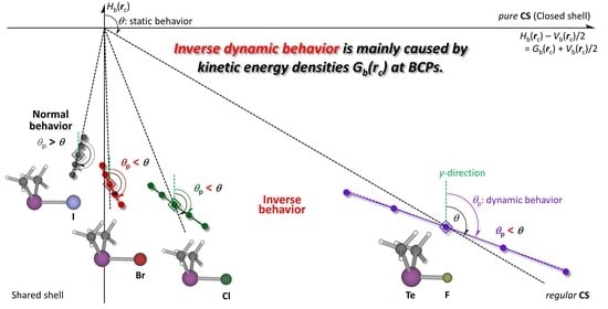
θp) = (202.8°, –0.2°). It is reasonable to assume that an interaction shows normal behavior if Δθp > 0, whereas it does the inverse behavior when Δθp < 0, which we propose in this work. Namely, all standard interactions in 136 behave normally, except for 35, which shows inverse behavior, although the magnitude of Δθp is very small. To elucidate the nature of the interactions based on the Δθp values, investigations are started by examining the basic trend in the standard interactions of 136, employing the Δθp values.
Figure 2 shows the plot of Δθp versus θ for 136 (Scheme 1). The plot is analyzed using a regression curve of the eighth-order function after the addition of some fictional points, such as (θ, Δθp) = (45°, 0°) and (206.6°, 0°), and omitting the data for 35 and Me2Se+-∗-Cl (26). Fortunately, a smooth regression curve, described by fθp), was obtained, and the curve passes very close to the points of (45°, 0°) and (206.6°, 0°). The regression curve is shown by a black solid line in Figure 2. The maximum point of the regression curve, shown by the solid line, was (θ, Δθp) = (109.7°, 48.9°). The regression curve was revised to a new curve by amplifying the maximum value of (109.7°, 48.9°) to (109.7°, 50.0°). The new curve is described by frθp) and shown by the dotted line. The treatment helps the discussion to be simpler, because the maximum value of 48.9° should be tentative and change depending on the employed species. Two more curves of frθp)/2 and −frθp)/2 are added in Figure 2, which are shown by the blue and red dotted lines, respectively, for a better explanation of the behavior.
The data for the normal behavior of the interactions with Δθp > 0 appear on the upper side of the x-axis in Figure 2. Interactions show inverse behavior if the (θ, Δθp) points appear downside of the x-axis. The typical data for the normal behavior of interactions should appear around the black dotted line of frθp), whereas data for the inverse behavior of interactions appear around the red dotted line of −frθp)/2. An interaction is called to show weak normal behavior if the point appears between frθp)/2 and the x-axis. The interaction in Ne-∗-HF (2) seems to show borderline to weak normal behavior (Figure 2). While the interactions in 26 are borderline between weak normal and inverse behavior, that in 35 show inverse behavior, close to weak normal behavior.
Very similar results were obtained in the plot of Δθp versus θ for 136 when calculated with BSS-B (see Table S4 and Figure S1 of the Supplementary Materials for the data calculated with BSS-B). The Δθp values are similarly plotted versus θ for the wide range of data of [Cl–Cl-∗-Cl] (16), calculated under aug-cc-pVTZ, where the perturbed structures of 16 are generated with POM. The plot is shown in Figure S2 of the Supplementary Materials, together with the data for 136. Figure A1 is essentially the same as Figure 2 (see Figure 1 for the QTAIM-DFA plot of 16, shown by the dotted line). A detailed comparison of the two figures revealed that the plots are very close to each other when the Cl-∗-Cl distances in question are longer than the optimized values, whereas the Δθp values for 16 are evaluated to be somewhat larger than those expected based on the data for 136 when the Cl-∗-Cl distances in question become shorter than the optimized values of 2.300 Å. When the interaction distance becomes shorter than the optimized value, the energy curve sharply tightens. The calculation conditions for POM under the interaction distances are widely shorter than the optimized values, where the shortened distance are 0.5 Å for 20 data points. The very severe conditions would be responsible for the results.
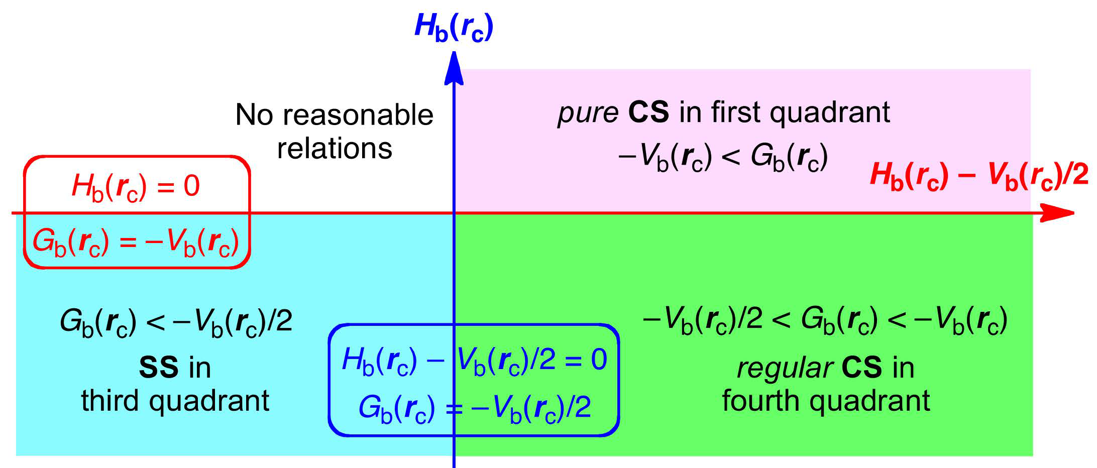
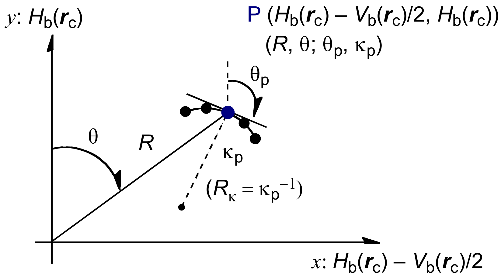
The close similarity between the two figures can be explained as follows: Starting from interatomic distances that are long enough, chemical bonds or interactions form as the distances shorten. The processes for the interactions are similar to each other, if the interactions of the normal behavior are compared. The processes can be understood based on the Hb(rc) and Hb(rc) − Vb(rc)/2 values or the plot of Hb(rc) versus Hb(rc) − Vb(rc)/2. In these cases, the (θ, θp) values are very close to each other, if they are calculated at the points of substantially the same positions on the plots. Namely, starting from interaction distances that are far enough, stable interactions form as if they go along the similar plot of Hb(rc) versus Hb(rc) − Vb(rc)/2. The drive on the plot arrives at a point of the minimum energy of the interaction, where the (θ, θp) values are given for the interaction. Different (θ, θp) values are obtained because the minimum energy is mainly determined depending on the interacting atoms. There must also be some differences in the energy curves, depending on the characteristics of the interactions, which result in the somewhat different curves of the plots. This should be the reason that the data points of various interactions appear close to the curve for the plot of (θ, Δθp) of 16.
The next investigation is to search for the interactions with negative Δθp values after the establishment of the basic trend in the normal behavior of the standard interactions.

3.2. Behavior of Various Interactions Based on θ and Δθp

Table 1 collects the Hb(rc) − Vb(rc)/2 and Hb(rc) values for 3761, similarly calculated under MP2/BSS-A’. Figure 3 shows the plots of Hb(rc) versus Hb(rc) − Vb(rc)/2 for the data of 3761 shown in Table 1, where the perturbed structures are generated with CIV. Contrary to the case of Figure 1, some plots for the interactions in Figure 3 show different streams from the main (averaged) stream, which must be a reflection of the different behaviors of the interactions. The (R, θ) and (θp, κp) values were similarly calculated for 3761 under MP2/BSS-A’. Table 1 collects the values, together with the Δθp and Cii values and the predicted natures. The Δθp values were plotted versus θ for the data of 3761 shown in Table 1. 
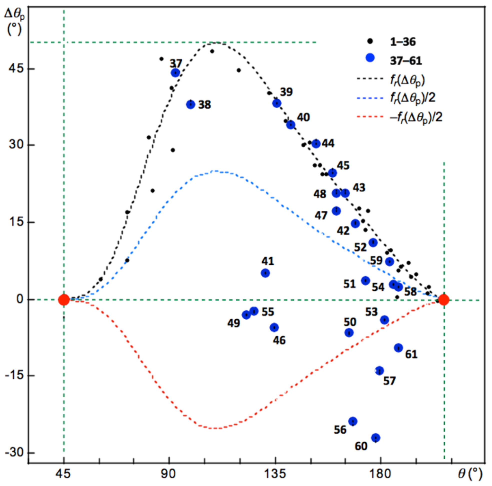
Figure 4 shows the plots.
As shown in Figure 4 (and Table 1), the data of the (θ, Δθp) values drop very near the frθp) curve for most of 3761, which shows the normal behavior of the interactions, although some points appear much further below the frθp) curve. The data of the (θ, Δθp) values appear between the frθp)/2 curve and the x-axis for Me2Te-∗-F2 (41; (θ, Δθp) = (131.0°, 5.0°)), Me2BrTe-∗-Br (51; (173.1°, 3.5°)), Me2Se+-∗-I (54; (185.0°, 2.9°)) and Me2Te+-∗-I (58; (187.3°, 2.3°)). The interactions show weak normal behavior. The (θ, Δθp) points appear between the x-axis and the −frθp)/2 curve for F-∗-IF (46; (θ, Δθp) = (134.5°, −5.5°)), Me2FTe-∗-F (49; (122.6°, −3.0°)), Me2ClTe-∗-Cl (50; (166.3°, −6.6°)), Me2S+-∗-I (53; (181.7°, −4.0°)) and Me2Te+-∗-F (55; (126.0°, −2.4°)), which show the inverse behavior of the interactions. In the case of Me2Te+-∗-Cl (56; θ, Δθp) = (168.0°, −23.9°)), Me2Te+-∗-Br (57; (179.5°, −14.0°)), H3C-∗-F (60; (177.6°, −27.0°)) and H3C-∗-I (61; (187.2°, −9.5°)), the data appear below the −frθp)/2 curve. Therefore, the interactions are recognized to show inverse behavior stronger than that supposed from the behavior of the standard interactions in 136.
What are the differences in the nature of the interactions among the three groups? The (θ, Δθp) values are examined in more detail for the interactions shown in Table 1. The typical (θ, Δθp) values for Me2Te-∗-X2 (4144), Me2(X)Te-∗-X (4952), Me2Te+-∗-X (5558) and H3C-∗-X (30, 31, 60, and 61) (X = F, Cl, Br, and I) are shown in Equations (12)–(15), respectively. The interactions in the equations are arranged in ascending order of Δθp.
(θ, Δθp) = (152.4°, 30.2°) for Me2Te-∗-I2 (44) > (164.7°, 20.6°) for Me2Te-∗-Br2 (43) >
(169.1°, 14.7°) for Me2Te-∗-Cl2 (42) > (131.0°, 5.0°) for Me2Te-∗-F2 (41)
(176.7°, 11.1°) for Me2(I)Te-∗-I (52) > (173.1°, 3.5°) for Me2(Br)Te-∗-Br (51) >
(122.6, −3.0°) for Me2(F)Te-∗-F (49) > (166.3°, −6.6°) for Me2(Cl)Te-∗-Cl (50)
(187.3°, 2.3°) for Me2Te+-∗-I (58) > (126.0°, −2.4°) for Me2Te+-∗-F (55) >
(179.5°, −14.0°) for Me2Te+-∗-Br (57) > (168.0°, −23.9°) for Me2Te+-∗-Cl (56)
(193.8°, 5.2°) for H3C-∗-Cl (30) > (191.8°, 4.5°) for H3C-∗-Br (31) >
(187.2°, −9.5°) for H3C-∗-I (61) > (177.6°, −27.0°) for H3C-∗-F (60)
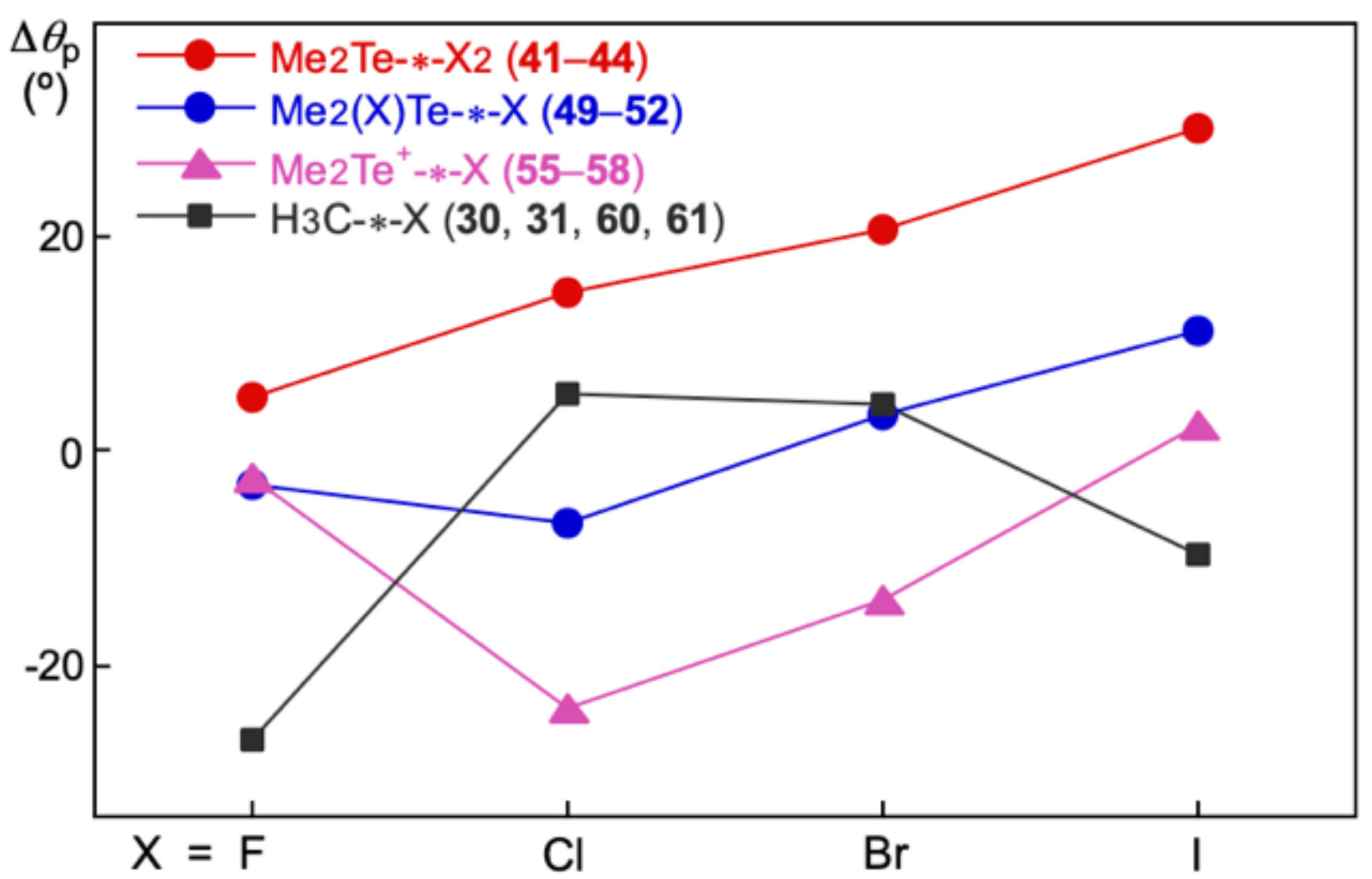
Figure 5 shows the plot of Δθp versus X (X = F, Cl, Br, and I) for 4144, 4952, 5558 and 30, 31, 60, and 61. The Δθp values for the interactions in 4144, 4952 and 5558 are in the order of Me2Te-∗-X2 > Me2(X)Te-∗-X > Me2Te+-∗-X, as a whole, if those of the same X are compared. The strength of Te–X is in the order of Me2Te-∗-X2 < Me2(X)Te-∗-X < Me2Te+-∗-X; therefore, the strength of Te–X in the species operates to decrease the Δθp values for the species.
The Δθp values for the interactions in 4144 become more positive, as X goes from F to Cl, then Br, and then to I, where the character (or atomic number) of X becomes closer to Te in 4144. The Δθp values in 4952 and 5558 show the trends, similar to that in 4144, for X = Cl, Br and I. The strength of Te–X operates to decrease the Δθp values also for the species. However, the Δθp values in 49 and 55 become more negative, when X goes F to Cl, contrary to the case in 41. The differences in the strength of Te–F in 41, 49 and 55 would result in smaller differences in the plot. In the case of H3C-∗-X, the Δθp values become more negative in the order of X = Cl ≥ Br > I >> F. The behavior of the interactions should be controlled by the differences in the characters (or atomic numbers) of X. The character of C in H3C-∗-X should be closer to those of Cl and Br, relative to the case of I and F. The calculated results are well explained based on Equations (5) and (6).
What are the behavior of the E-∗-E’ bonds in the neutral, monoanionic, monocationic, and dicationic forms of [MeE-∗-E’Me]* (E, E’ = S, Se, and Te; * = null, −, +, and 2+)? The species are optimized, first. The optimized structures of the neutral form have C2 symmetry for E = E’ and close to C2 symmetry for E ≠ E’. Here, the structures are called the C2 type. The structures of the C2 and trans types are optimized for the monoanionic form. The structures of the C2 type are only discussed here because the Δθp values are larger than 20° for both forms (Table 2). The structures of the trans type are optimized for the mono- and dicationic forms. Table 2 collects the (θ, θp, Δθp) values of the species calculated under MP2/BSS-C. Numbers for the species are shown in Table 1. The calculated results, other than those in Table 2, are collected in Table S8 of the Supplementary Materials.
The behavior of the interactions is examined next, based on the (θ, Δθp) values. Positive Δθp values of 28.2–32.3° are predicted for the monoanionic forms of [MeE-∗-E’Me] (E, E’ = S, Se and Te) shown in Table 2. Positive Δθp values (2.6–6.8°) are predicted for S-∗-S, S-∗-Se, Se-∗-Se and Te-∗-Te of the neutral, mono- and dicationic forms of [MeE-∗-E’Me]* (E, E’ = S, Se, and Te; * = null, +, and 2+). However, negative Δθp values are predicted for the neutral forms of MeS-∗-TeMe (Δθp = −14.2°) and MeSe-∗-TeMe (−3.7°); the monocationic forms of [MeS-∗-TeMe]+ (c−15.5°) and [MeSe-∗-TeMe]+ (−3.9°); and the dicationic forms of [MeS-∗-TeMe]2+ (−11.3°) and [MeSe-∗-TeMe]2+ (−3.2°).
Se-∗-Se (6.6 ≤ Δθp ≤ 6.8°) > S-∗-S (5.5°–5.8°) > S-∗-Se (2.6–6.5°) > Te-∗-Te (2.7–3.2°) >
Se-∗-Te (−3.7 − −3.2°) > S-∗-Te (−15.5 − −11.3°)
Equation (16) shows the common order for Δθp of E-∗-E’ in the neutral, mono- and dicationic forms of [MeE-∗-E’Me]* (E, E’ = S, Se, and Te), where the equation is arranged in the ascending order of Δθp. The order can also be understood under the guidance of the conclusions derived from Equations (5) and (6). That is, the Δθp values are more negative as the difference in the atomic numbers of A and B in A-∗-B becomes larger. However, it is not so clear that the Δθp values for the same A-∗-B become more negative if the interaction in question becomes stronger.
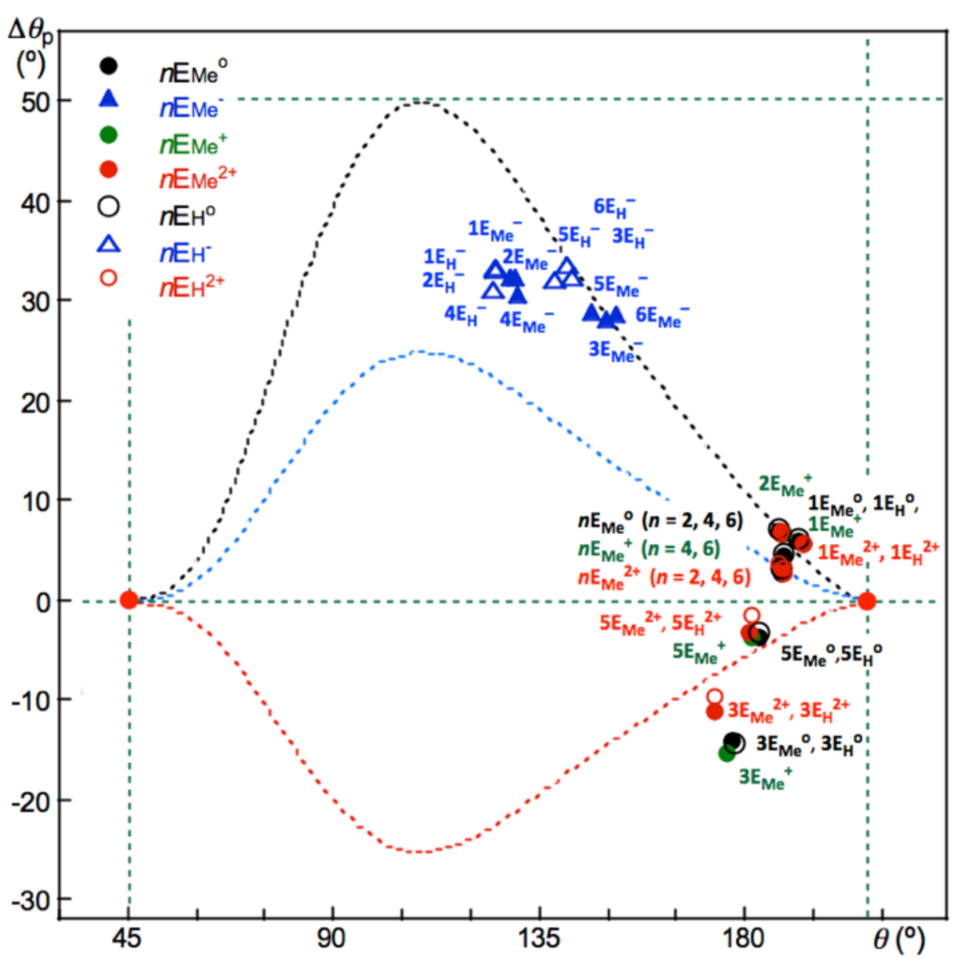
Figure 6 shows the plot of Δθp versus θ for the E-∗-E’ interactions in the neutral, monoanionic, monocationic and dicationic forms of [MeEE’Me]* (E, E’ = S, Se and Te; * = null, −, + and 2+). (See Table 2 for the values). The normal, weak normal and inverse behavior of interactions is clearly illustrated in the figure. A very similar trend is observed in the neutral, anionic and dicationic forms of [HE-∗-E’H]* (E, E’ = S, Se and Te; * = null, − and 2+). The calculated results are collected in Table S8 of the Supplementary Materials, and the values are plotted in Figure 6. Some (data) points of (Δθp, θ) appear below the –frθp)/2 curve for S-∗-Te in 3EMe0, 3EH0, 3EMe+ and 3EMe2+, and 3EH2+ with Se-∗-Te in 5EMe0 and 5EH0. The results show that some S-∗-Te and Se-∗-Te interactions show stronger inverse behavior than that supposed from the behavior for the standard interactions in 136.
The behavior of E-∗-E’ in [HE-∗-E’H]* (E, E’ = S, Se and Te; * = null, − and 2+) is very similar to the behavior in [MeE-∗-E’Me]* (E, E’ = S, Se and Te; * = null, −, + and 2+); therefore, the behavior of E-∗-E’ in [HE-∗-E’H]* (E, E’ = S, Se and Te; * = null, −, + and 2+) is not discussed in detail here. Nevertheless, the behavior of [HS-∗-TeH]2+ is discussed later.
The (θ, θp, Δθp) values for E-∗-C and E’-∗-C, together with E-∗-H and E’-∗-H, in [REE’R]* (R = Me and H: E, E’ = S, Se, and Te; * = null, −, +, and 2+) are collected in Table S8 of the Supplementary Materials. 
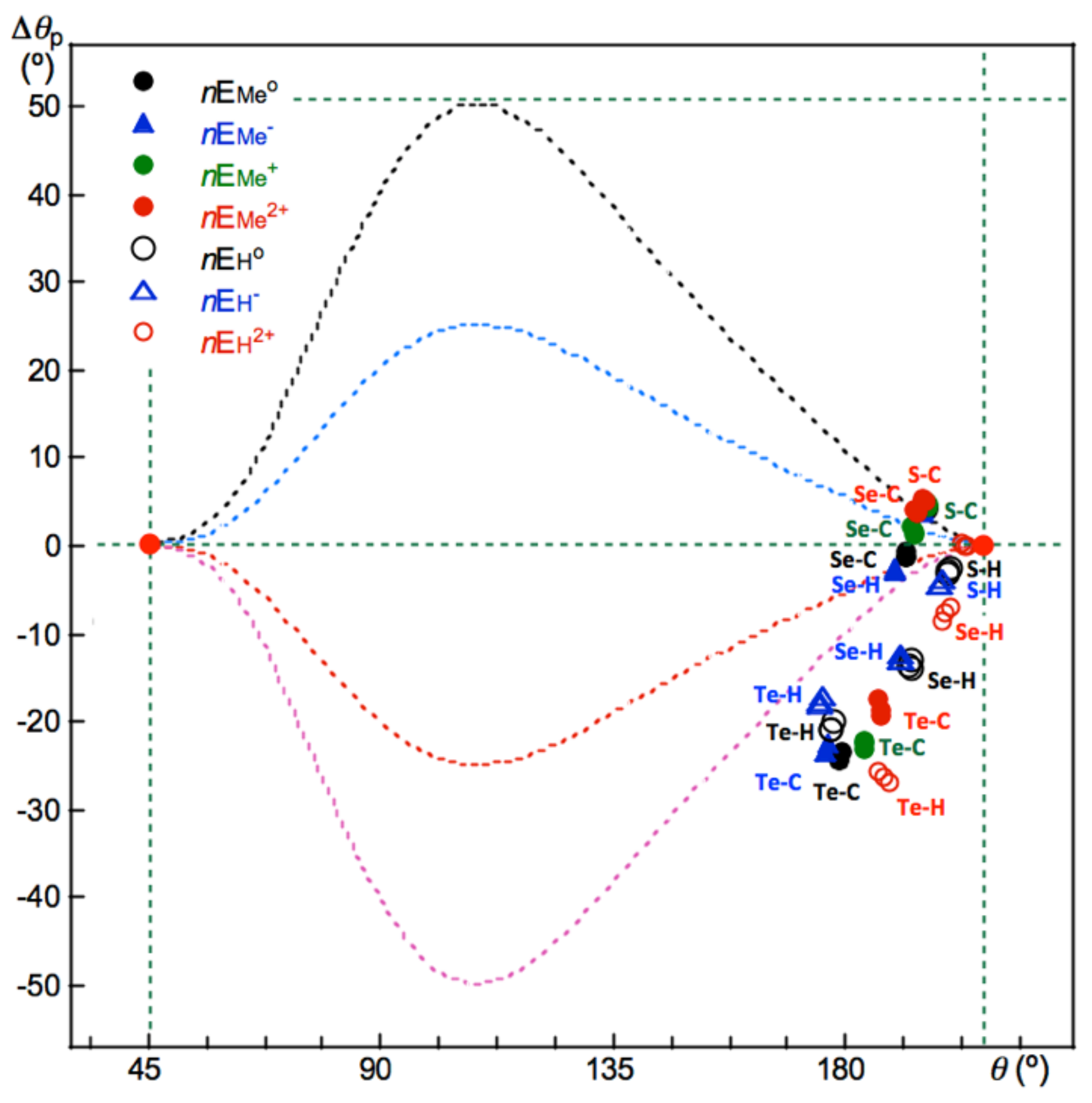
Figure 7 shows the plot of Δθp versus θ, for the data in Table S8. A lot of data are well visualized.
As shown in the table and the figure, the Δθp values are negative for Te-∗-C in MeETe-∗-Me (E = S, Se and Te: −24.5° ≤ Δθp ≤ −23.5°), [MeETe-∗-Me] (E = S, Se and Te: −23.5° ≤ Δθp ≤ −22.5°), [MeETe-∗-Me]+ (E = S, Se and Te: −23.1° ≤ Δθp ≤ −22.3°), and [MeETe-∗-Me]2+ (E = S, Se and Te: −19.4° ≤ Δθp ≤ −17.3°), whereas the values are all positive for S-v-C of [Me-∗-SE’Me]* (E’ = S, Se and Te; * = null, –, + and 2+: 3.9° ≤ Δθp ≤ 5.4°). In the case of Se-∗-C, the Δθp values are negative for MeESe-∗-Me (E = S, Se and Te: −1.4° ≤ Δθp ≤ −0.7°) and [MeESe-∗-Me] (E = S, Se and Te: −2.8° ≤ Δθp ≤ −2.5°), whereas the values are positive for [MeESe-∗-Me]+ (E = S, Se and Te: 1.4° ≤ Δθp ≤ 2.2°) and [MeESe-∗-Me]2+ (E = S, Se and Te: 3.7° ≤ Δθp ≤ 4.1°). The Δθp values of E-∗-C and E’-∗-C are plotted in [Me-∗-EE’-∗-Me]* (E, E’ = S, Se and Te; * = null, −, + and 2+), containing the values from the symmetric [Me-∗-EE-∗-Me]* (E = S, Se and Te; * = null, −, + and 2+). In the case of E-∗-H and E’-∗-H, the Δθp values are negative for all S-∗-H, Se-∗-H, and Te-∗-H shown in the table. The Δθp values are −4.5° ≤ Δθp ≤ −2.5° for HES-∗-H and [HES-∗-H], −13.9° ≤ Δθp ≤ −12.2° for HESe-∗-H and [HESe-∗-H] and −20.9° ≤ Δθp ≤ −17.1° for HETe-∗-H and [HETe-∗-H], where E = S, Se and Te. Most of the (data) points of (Δθp, θ) for E-∗-H (E = S, Se, and Te) and Te-∗-H appear below the −frθp) curve, tentatively drawn in the plot. The interactions show much severer the inverse behavior is than that supposed from the behavior for the standard interactions of 136.
After recognizing the interactions with Δθp < 0, the next extension is to clarify the origin and mechanisms that cause the negative Δθp values.

3.3. Requirements for the Positive to Negative Values of Δθp for the Interactions in Question

The Δθp value for an interaction is Δθp > 0, Δθp = 0 or Δθp < 0, depending on the dynamic nature of the interaction. The dynamic nature was considered based on the characteristics of the plot around the BCP. Figure 8 illustrates the requirements for the QTAIM-DFA plot of Hb(rc) versus Hb(rc) − Vb(rc)/2, where the arrows on the plot lines indicate the direction in which the interaction distance becomes shorter. As shown by the black plot in Figure 8, the Δθp value for an interaction is positive when its plot line crosses the line for θ in the direction of clockwise rotation, viewed from the origin. The Δθp value is negative when its plot line crosses the line for θ in the direction of counterclockwise rotation. The Δθp value is zero when it is parallel to the line for θ, as shown by the blue plot.

3.4. Processes to Arise the Negative Δθp Values around the Optimized Structures

The processes to give the negative Δθp values are examined for some interactions from the sufficiently distant states to around the optimized structures. Hb(rc) values are plotted versus Hb(rc) − Vb(rc)/2 for the reaction processes over wide ranges of the interaction distances in question. It is more suitable if the singlet state is retained throughout the process, which relieves us from the trouble of considering the effect of the change on the multiplicity in the process. The structural change is also expected to be limited to the minimum extent if the singlet state is retained throughout the processes. The analysis is much simpler under these conditions, together with the discussion. As a result, the mechanisms to give the negative Δθp values are more clearly understood as the reactions proceed if the singlet state is retained throughout the reaction processes. Such processes seem rather rare and satisfy the above conditions.
The negative Δθp value of −4.2° is calculated for [F–I-∗-F] (46), as shown in Table 1, where the reaction process is shown by Equation (17). The reaction shown by Equation (18) has been reported to proceed in the singlet state under metal-free conditions [19,20]. A negative value of −22.8° was also calculated for Tf–N-∗-IMe (Tf = SO2CF3) (Table 3). The reaction processes for [F–I-∗-F] (46) in Equation (17) and Tf–N-∗-IMe in Equation (18) could be good candidates to achieve this purpose. Therefore, the reaction processes to give the negative Δθp values are examined, exemplified by the reactions shown in Equations (17) and (18).
F–I + F → [F–I-∗-F]
Tf–N-∗-BrMe + MeI → TS [MeBr-∗-N(Tf)-∗-IMe] → MeBr + Tf–N-∗-IMe
Tf–N-∗-BrMe + MeBr → TS [MeBr-∗-N(Tf)-∗-BrMe] → MeBr + Tf–N-∗-BrMe
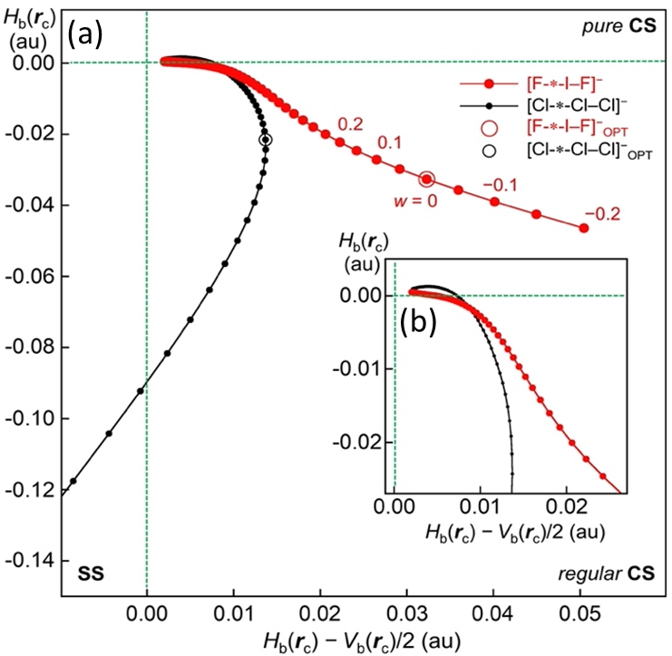
Figure 9 shows the QTAIM-DFA plot of Hb(rc) versus Hb(rc) − Vb(rc)/2 for [F–I-∗-F] for a wide range of the interaction distances in question. Fortunately, the perturbed structures were successfully (and easily) obtained for a wide range of interaction distances under MP2/BSS-C. Figure 9 contains the plot for [Cl–Cl-∗-Cl], similarly calculated, for comparison (see also Table 1). The plot for [Cl–Cl-∗-Cl]
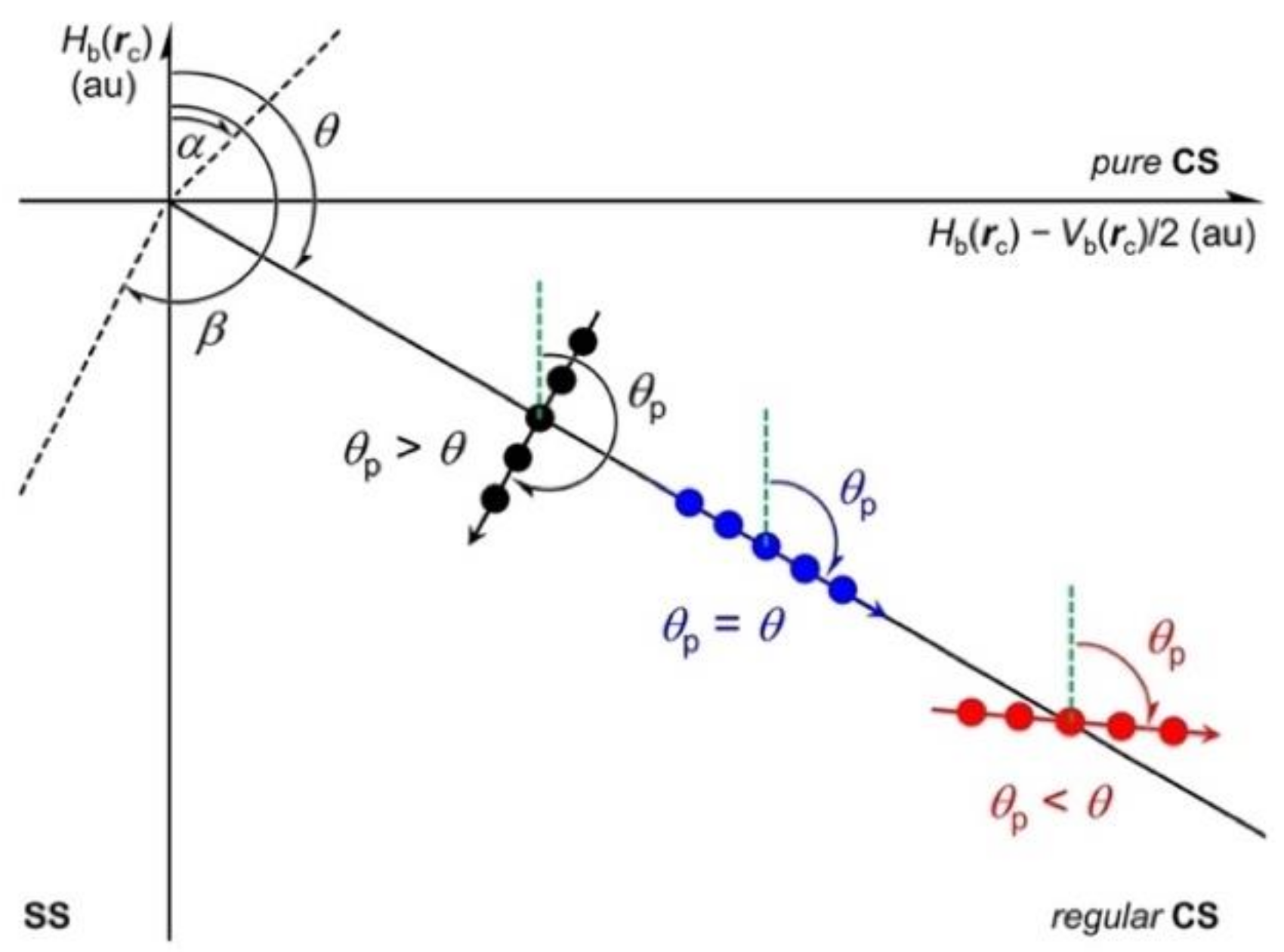
 shows a smooth and monotonic curve, starting from a point close to the origin. The plot for [Cl–Cl-∗-Cl] forms a spiral curve overall. As a result, the curve of the plot for [Cl–Cl-∗-Cl] satisfies the requirements for θp > θθp > 0) throughout the reaction process, as illustrated in Figure 9. This is the reason that [Cl–Cl-∗-Cl] typically shows the normal behavior of interactions.
However, the plot for [F–I-∗-F] seems different from the plot for [Cl–Cl-∗-Cl] in some points. The plot does not show the spiral figure as a whole. The plot of [F–I-∗-F] seems similar to the plot of [Cl–Cl-∗-Cl] when Hb(rc) − Vb(rc)/2 < 0.01 au, as shown in the magnified Figure 9b. However, the plots for the two interactions become much different if Hb(rc) − Vb(rc)/2 > 0.02 au. The Hb(rc) value seems to decrease almost linearly as the Hb(rc) − Vb(rc)/2 value becomes larger, especially for the range of Hb(rc) − Vb(rc)/2 > 0.02 au. The plot for [F–I-∗-F] seems to show a downwardly convex character for the range, which is very different from the plot for [Cl–Cl-∗-Cl]. The characteristic figure in the plot for [F–I-∗-F] prevents us from showing the spiral stream. The curve for the plot of [F–I-∗-F] would satisfy the requirements for θp > θθp > 0) in the range of Hb(rc) − Vb(rc)/2 < 0.02 au, as illustrated in Figure 9. The curve gradually changes to show the downwardly convex character to satisfy the requirements for θp = θθp = 0). The optimized structure, shown by w = 0.0 in Figure 9, appears in the range satisfying the requirements for θp < θθp < 0), illustrated in Figure 8. Indeed, the plot in Figure 9 shows the outline to give the negative Δθp value (–5.5°) for [F–I-∗-F] (46), but it is better if the requirement for Δθp < 0 is illustrated more clearly in the plot for a process. Next, this process was examined and exemplified by the ligand exchange reaction at N via TS [MeBr-∗-N(Tf)-∗-IMe].
Table 3 collects the (θ, θp, Δθp) values for the interactions of Tf–N-∗-BrMe, Tf–N-∗-IMe and TS [MeBr-∗-N(Tf)-∗-IMe], which have been calculated at the BCPs under MP2/BSS-C’. Table 3 contains the values for TS [MeBr-∗-N(Tf)-∗-BrMe], similarly calculated, for reference. The perturbed structures were calculated in the processes shown in Equations (17) and (18) with the IRC method, starting from TS [MeBr-∗-N(Tf)-∗-IMe] and TS [MeBr-∗-N(Tf)-∗-BrMe]. The perturbed structures of the Br-∗-N and N-∗-I interaction distances of wide ranges could be successfully calculated with the IRC method under MP2/BSS-C’.
The reaction processes shown in Equation (19) were examined before investigations on those shown in Equation (18). Hb(rc) is plotted versus Hb(rc) − Vb(rc)/2 for both Br-∗-N bonds in the ligand exchange reaction via TS [MeBr-∗-N(Tf)-∗-BrMe]. The plot is shown in Figure S3 of the Supplementary Materials, consisting of two plots, very close to each other, because TS [MeBr-∗-N(Tf)-∗-BrMe] has no symmetry due to the slightly different geometry around the Br-∗-N-∗-Br moiety. Therefore, the nature of Br-∗-N on both sides of the TS [MeBr-∗-N(Tf)-∗-BrMe] is slightly different. The Δθp values are calculated to be 50.3° and 49.1° for TS [MeBr-∗-N(Tf)-∗-BrMe], respectively.
The plots for the two N-∗-Br interactions via TS [MeBr-∗-N(Tf)-∗-BrMe] show a smooth, monotonic and spiral curve, very similar to the curve for [Cl–Cl-∗-Cl] (Figure 1 and Figure 9). Consequently, both Br-∗-N are recognized to show the typical normal behavior of interactions, which leads to positive Δθp values for the final products. The Δθp values of the final products of MeBr-∗-N–Tf and the isomer are 7.4° and 5.8°, respectively, depending on slight differences in the geometry. The similarity in the reaction processes between MeBr-∗-N–Tf and [Cl-∗-Cl-∗-Cl] is of significant interest. The processes proceed in both directions and give the final products from TS [MeBr-∗-N(Tf)-∗-BrMe] of the highest energy for the former but from the global minimum of the lowest energy for the latter.
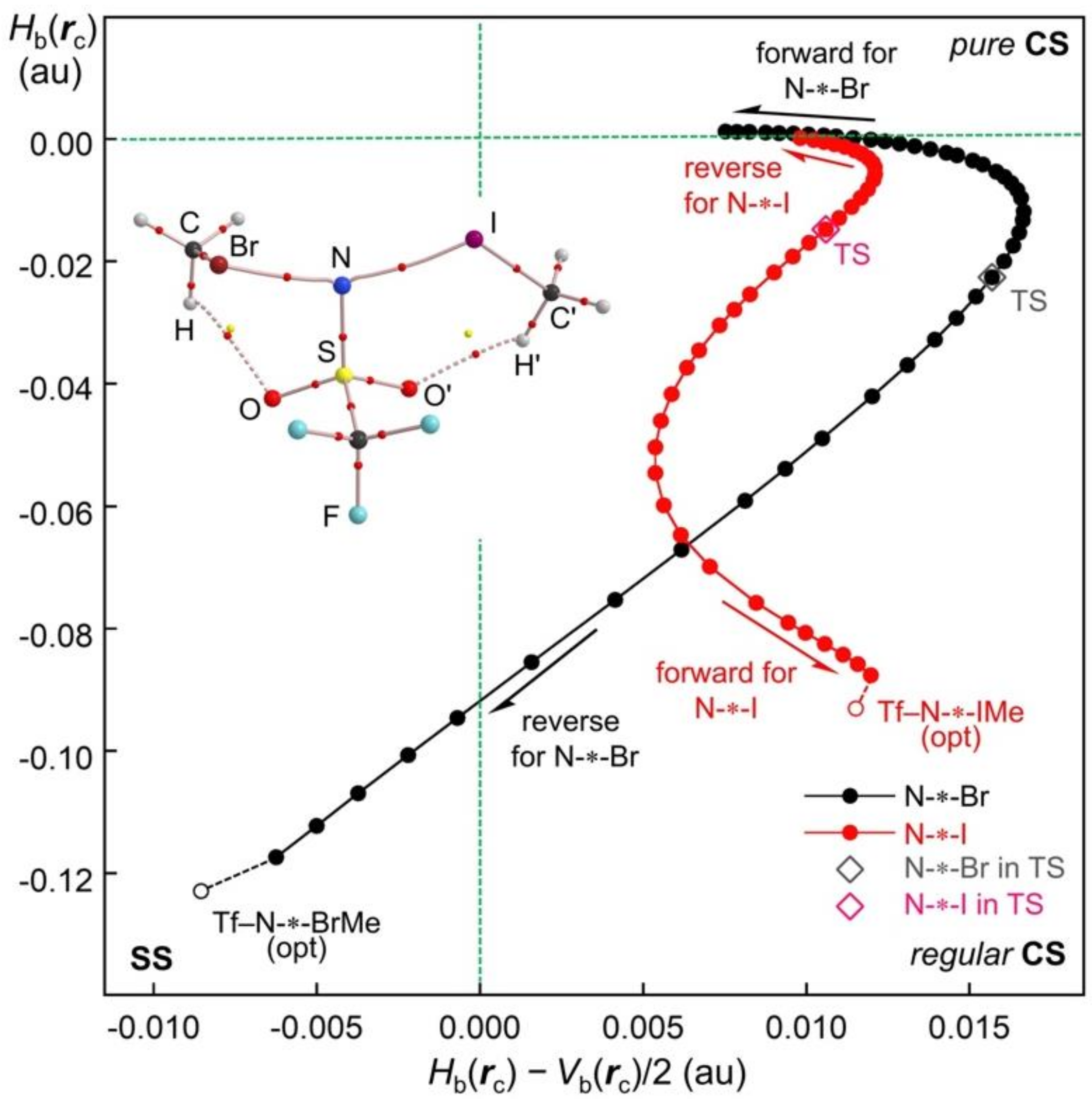
Figure 10 shows the QTAIM-DFA plots for the process shown by Equation (18). Figure 10 is briefly explained to avoid misunderstanding. It is not a plot for the energy profile, but a QTAIM-DFA plot for both Br-∗-N and N-∗-I, so two plots appear corresponding to the two bonds, while a single transition state contributes to the reaction. (This is also the case for the plots in Figure S3 of the Supplementary Materials.) The forward and reverse processes for the reaction shown by Equation (18) are clearly specified in Figure 10.
In spite of the forward and reverse processes for the reaction, the plot for Br-∗-N is drawn by the black dots in Figure 10, which corresponds to the reaction process of Equation (18). The process forms MeI + Tf–N-∗-BrMe, starting from Tf–N-∗-IMe + MeBr via TS [MeBr-∗-N(Tf)-∗-IMe]. The Δθp value of Br-∗-N changes from 7.9° for Tf–N-∗-BrMe to 42.6° for TS [MeBr-∗-N(Tf)-∗-IMe], then to 0.0°, with no interaction state, if the reaction proceeds in the direction shown in Equation (18).
The plot for Br-∗-N in Figure 10 also shows a smooth, monotonic and spiral curve, which is very similar to the curve for [Cl–Cl-∗-Cl] (Figure 1 and Figure 9) and the curves for Br-∗-N illustrated in Figure S3 of the Supplementary Materials (see Equation (19)). Consequently, the Br-∗-N bond in the ligand exchange reactions via TS [MeBr-∗-N(Tf)-∗-IMe] shows normal behavior similar to the case of TS [MeBr-∗-N(Tf)-∗-BrMe] and [Cl–Cl-∗-Cl]. However, the plot for I-∗-N in Figure 10 is drawn by the red dots. The process forms MeBr + Tf–N-∗-IMe, starting from Tf–N-∗-BrMe + MeI via TS [MeBr-∗-N(Tf)-∗-IMe]. The Δθp value of I-∗-N goes from 0.0° for MeI to 48.4° for TS [MeBr-∗-N(Tf)-∗-IMe], then to −22.8° for Tf–N-∗-IMe if the reaction proceeds in the direction shown in Equation (18). The plot for I-∗-N is very different from the plot for N-∗-Br, as shown in Figure 10. The difference between the plots clarifies the mechanism to give the negative Δθp value for Tf–N-∗-IMe.
The plot for N-∗-I in red shows a distorted Z shape. This is of great interest because the plot for N-∗-I seems to largely overlap the plot for N-∗-Br in the range of Hb(rc) > −0.02 au, if the plot for N-∗-I is moved to the right. The plot for N-∗-I curves to the left in the range of −0.05 < Hb(rc) < −0.006 au, then crosses the plot for N-∗-Br at Hb(rc) around −0.07 au. The plot for N-∗-I shows a downward-sloping linear shape in the range of Hb(rc) < –0.08 au. The mechanism to cause the negative Δθp value for Tf–N-∗-IMe, based on the characteristic figure in the plot of N-∗-I shown in Figure 10, can be explained as follows: The Δθp value for N-∗-I in the reaction, shown in Equation (18), must be positive if Hb(rc) > −0.06 au for N-∗-I, starting from Tf–N-∗-BrMe + MeI (no interaction between N and I). The positive Δθp value decreases for the plot curving to the left in the range of −0.05 < Hb(rc) < −0.01 au, then approaches zero, and finally gives the negative Δθp value of −12.9° for Tf–N-∗-IMe in the range of Hb(rc) < −0.09 au.
In the plot for N-∗-I in Figure 10, Hb(rc) decreases monotonically, whereas Hb(rc) – Vb(rc)/2 shows abnormal behavior when Hb(rc) < 0. Therefore, it is strongly suggested that the strange behavior of Hb(rc) – Vb(rc)/2 should be responsible for the negative Δθp value.
The process for N-∗-I to give the negative Δθp value is well clarified by the plot for N-∗-I in Figure 10. However, it would be difficult to visually recognize the value of Δθp, positive or negative, from the plot. We searched for a typical example that can be recognized as a clear negative Δθp value visually from the plot. The (θ, θp, Δθp) values for [HS-∗-TeH]2+ are given in Table S8 of the Supplementary Materials, of which Δθp is a negative value of −9.7°. The process for [HS-∗-TeH]2+ was calculated with POM by elongating the S-∗-Te distance, starting from the structure around the optimized one. The calculations were performed in the range where the rational structures were optimized at the singlet state.
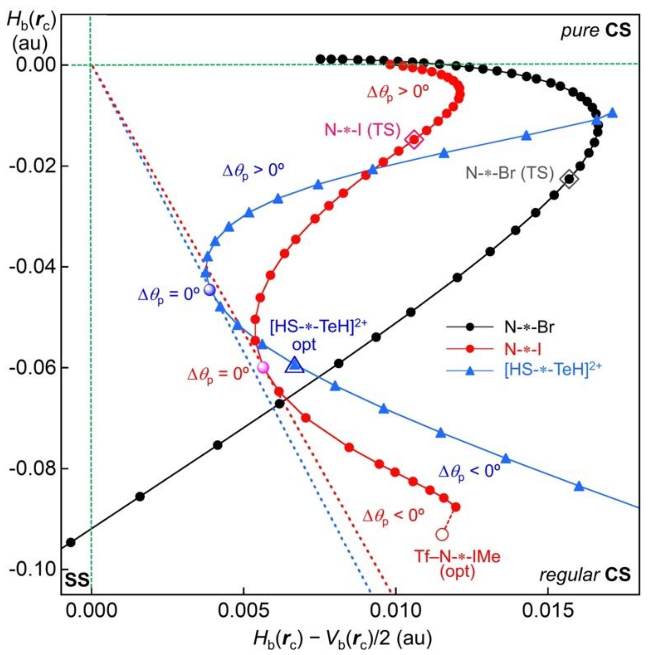
Figure 11 draws the reaction process for [HS-∗-TeH]2+, although the interaction distance is limited to the distance around the optimized structure, where the perturbed structures are rationally optimized at the singlet state. The plots for N-∗-I and N-∗-Br in the reaction processes shown in Equation (18) are added to Figure 11 for reference. The partial plot for [HS-∗-TeH]2+, shown in Figure 11, seems to correspond to the plot for N-∗-I in the range of Hb(rc) < −0.005 au. The lines of Δθp = 0° for the plots of N-∗-I and [HS-∗-TeH]2+ are drawn by the red and blue dotted lines, respectively. The tangent directions from the origin to the curves correspond to the lines of Δθp = 0° (see also Figure 8).
As discussed above, the plot for N-∗-Br satisfies the requirement for Δθp > 0° in the whole range of the reaction process, while the plot for N-∗-I should satisfy the requirement for Δθp < 0° around the optimized structure. However, it seems visually unclear from the plot, as mentioned above. In the case of the plot for [HS-∗-TeH]2+, there exists an area that clearly satisfies the requirements for Δθp < 0°, after the blue dotted line for Δθp = 0°. The area with Δθp < 0° is the area around the optimized structure in this case. The crossing point on the plot with the tangent line corresponds to Δθp = 0°; therefore, the perturbed structure of which the S-∗-Te distance is shorter than the value at Δθp = 0° should show positive Δθp values, namely the area of Δθp ≥ 0°.
After clarification of the origin for the positive and negative Δθp values through the plots, the next extension is to elucidate the mechanisms based on the behavior of Gb(rc) and Vb(rc).

3.5. Mechanisms for the Origin of the Negative Δθp Values

The reaction processes can be directly expressed using the interaction distances. However, the ρb(rc) values can also be used for the analyses, where the values decrease exponentially as the interaction distances increase. The distances are also expressed by w in Equation (10). The relation between ρb(rc) and w is confirmed by the plot of ρb(rc) versus w for an interaction. Such a plot is shown in Figure S6 of the Supplementary Materials, exemplified by [Cl–Cl-∗-Cl] and [F–I-∗-F]. As a result, ρb(rc) would be the better parameter to describe the characteristics of interactions around the optimizes structures, in more detail, relative to the case of r and w for the longer distances. The characteristic behavior of Hb(rc) versus Hb(rc) − Vb(rc)/2 can be attributed to the behavior of Gb(rc) and Vb(rc), because Hb(rc) and Hb(rc) − Vb(rc)/2 are expressed by Gb(rc) and Vb(rc) (see Equations (1) and (2)). The reaction processes are investigated employing the plots of Hb(rc) − Vb(rc)/2, Hb(rc), Gb(rc) and Vb(rc) versus ρb(rc) and the related plots.
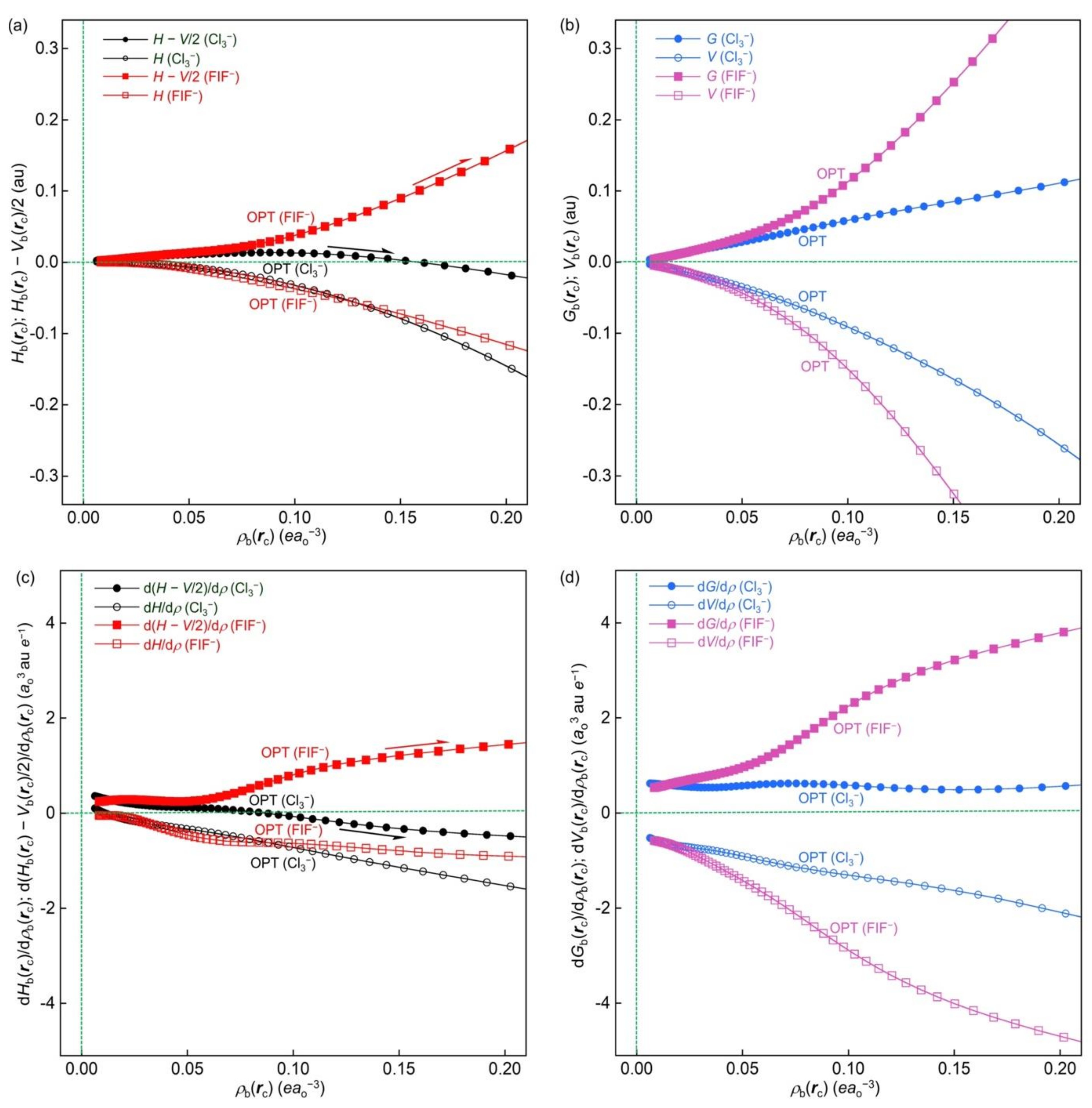
Figure 12a,b shows the plots of Hb(rc) − Vb(rc)/2, Hb(rc), Gb(rc) and Vb(rc) versus ρb(rc) for the reaction processes of [Cl–Cl-∗-Cl] and [F–I-∗-F], where the perturbed structures are generated with POM over the wide range of w. The plots of Gb(rc) versus ρb(rc) and Vb(rc) versus ρb(rc) for [Cl–Cl-∗-Cl] go upside and downside, respectively, very smoothly and monotonically, starting from a point close to the origin. The plot of the former goes upside almost linearly, while that of the latter goes downside, showing a slight convex upward shape. The magnitude of the former seems close to but less than two times the magnitude of the latter for the range of ρb(rc) < 0.16 (e/a03). The plots of Hb(rc) − Vb(rc)/2 versus ρb(rc) and Hb(rc) versus ρb(rc) are also smooth and gentle for [Cl–Cl-∗-Cl]. The Hb(rc) − Vb(rc)/2 value is positive and then negative after ρb(rc) ≥ 0.16 (e/a03), while the positive Hb(rc) becomes negative when ρb(rc) reaches approximately 0.026 (e/a03), leading to the normal behavior of the [Cl–Cl-∗-Cl] interactions (Δθp > 0). The plot of Hb(rc) versus Hb(rc) − Vb(rc)/2 for [Cl–Cl-∗-Cl] shown in Figure 9 is well explained through the plots of Hb(rc) − Vb(rc)/2 versus ρb(rc) and Hb(rc) versus ρb(rc) shown in Figure 12a.
In the case of [F–I-∗-F], the plots of Gb(rc) versus ρb(rc) and Vb(rc) versus ρb(rc) go upside and downside, respectively, smoothly and monotonically, starting from a point close to the origin. However, the plots show convex upward and downward shapes, respectively, and the magnitude of the former seems 0.8 times larger than the magnitude of the latter. As a result, the plot of Hb(rc) − Vb(rc)/2 versus ρb(rc) is mainly controlled by the plot of Gb(rc) versus ρb(rc), whereas the plot of Hb(rc) versus ρb(rc) is almost controlled by the plot of Vb(rc) versus ρb(rc) (cf; Equations (1) and (2)). Hb(rc) − Vb(rc)/2 and Hb(rc) are positive and negative in the calculated whole range for [F–I-∗-F], except for Hb(rc) of the substantially large range of r where ρb(rc) is substantially very small. Therefore, the plot of Hb(rc) versus Hb(rc) − Vb(rc)/2 is close to the linear relationship of the y = −ax (a > 0) type, which essentially explains the plot for [F–I-∗-F], as shown in Figure 9. The character of Gb(rc) versus ρb(rc) remains in the character of Hb(rc) − Vb(rc)/2 versus ρb(rc) for [F–I-∗-F]. The negative Δθp value of [F–I-∗-F] must arise from the characteristic plot of Hb(rc) versus Hb(rc) − Vb(rc)/2, which is close to the linear relationship of the y = −ax (a > 0) type, which originates from the characteristic plot of Hb(rc) versus Gb(rc).
Figure 12c,d show the plots of d(Hb(rc) − Vb(rc)/2)/dρb(rc), dHb(rc)/dρb(rc), dGb(rc)/dρb(rc) and dVb(rc)/dρb(rc) versus ρb(rc) for the reaction process of [Cl–C-∗-Cl] and [F–I-∗-F]. All plots seem almost linearly flat, except for the plots of d(Hb(rc) − Vb(rc)/2)/dρb(rc), dGb(rc)/dρb(rc) and dVb(rc)/dρb(rc) for [F–I-∗-F]. The results for F–I-∗-F] expose the behavior in the plot of d(Hb(rc) − Vb(rc)/2)/dρb(rc) versus ρb(rc). The behavior of the plot of Hb(rc) − Vb(rc)/2 versus ρb(rc) is shown to be the main factor leading to the negative Δθp value for F–I-∗-F], as expected.
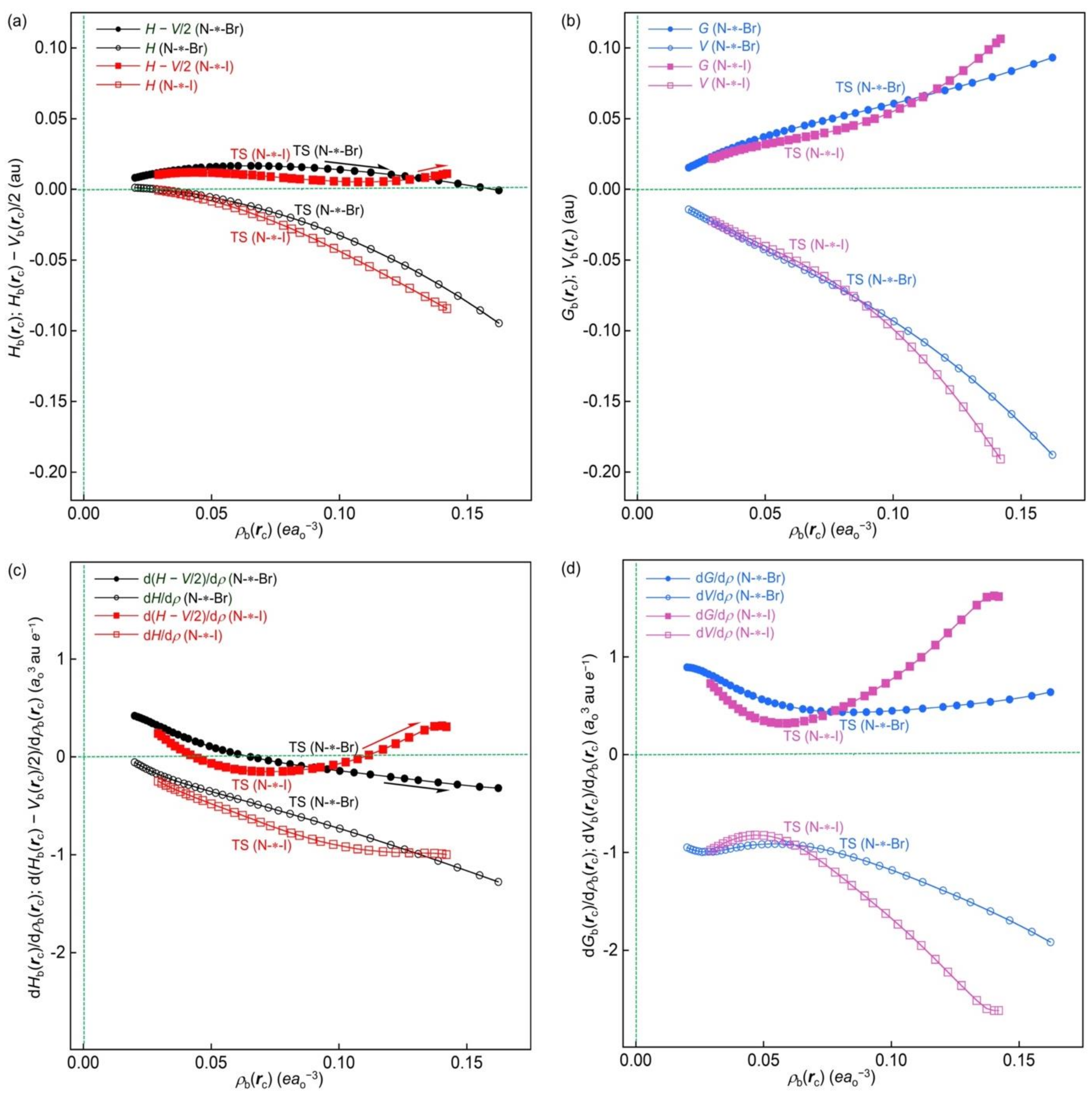
Figure 13a,b illustrate the plots of Hb(rc) − Vb(rc)/2, Hb(rc) Gb(rc) and Vb(rc) versus ρb(rc) for N-∗-Br and N-∗-I in the reaction processes from TS [MeBr-∗-N(Tf)-∗-IMe], where the perturbed structures are generated with the IRC method (see Equation (18)).
The plots of Hb(rc) − Vb(rc)/2, Hb(rc), Gb(rc), and Vb(rc) versus ρb(rc) for N-∗-Br are very similar to the corresponding plots for [Cl–C-∗-Cl], although the magnitudes of the plots are different. Consequently, the plot of Hb(rc) versus Hb(rc) − Vb(rc)/2 for N-∗-Br should be very similar to the plot for [Cl–C-∗-Cl]. The plot for N-∗-Br is well explained based on the analyzed results discussed above.
However, the plots of Gb(rc) versus ρb(rc) and Vb(rc) versus ρb(rc) for N-∗-I go upside and downside, respectively, starting from a point close to the origin. The plot of Gb(rc) versus ρb(rc) for N-∗-I gives a distorted Z-shaped curve, while the plot of Vb(rc) versus ρb(rc) shows a slightly distorted Z-shaped character. The magnitude of the plot of Gb(rc) versus ρb(rc) seems to be 0.7 times the magnitude of Vb(rc) versus ρb(rc) for N-∗-I. Therefore, the plot of Hb(rc) − Vb(rc)/2 versus ρb(rc) is controlled by the plot of Gb(rc) versus ρb(rc), whereas the plot of Hb(rc) versus ρb(rc) is controlled by the plot of Vb(rc) versus ρb(rc). Hb(rc) − Vb(rc)/2 and Hb(rc) are positive and negative in the whole range calculated for N-∗-I, except for Hb(rc) of the substantially very small range ρb(rc). Therefore, the plot of Hb(rc) versus Hb(rc) − Vb(rc)/2 appears in the regular CS region, except for the region of Hb(rc) > 0, very close to the origin. The character of Gb(rc) versus ρb(rc) remains in the plot of Hb(rc) − Vb(rc)/2 versus ρb(rc) for N-∗-I, again. The positive value of Hb(rc) becomes negative at approximately 0.028 (e/a03) for ρb(rc), and then the value becomes more negative as ρb(rc) becomes larger.
In the case of Hb(rc) − Vb(rc)/2, the value is positive in the whole region calculated for N-∗-I (Figure 13a). The plot of Hb(rc) − Vb(rc)/2 versus ρb(rc) for N-∗-I gives a rather clear distorted Z-shaped curve. The plot goes upside after the start of the plot at around the origin, then it goes downside and then goes upside. Consequently, the Z-shaped figure of Hb(rc) versus Hb(rc) − Vb(rc)/2 for N-∗-I shown in Figure 10 is well analyzed based on the characteristic behavior of the plot of Hb(rc) − Vb(rc)/2 versus ρb(rc), together with the plot of Hb(rc) versus ρb(rc). The abnormal behavior of Hb(rc) − Vb(rc)/2, derived from the abnormal behavior of Gb(rc), must be responsible for the negative Δθp value of N-∗-I in CF3SO2N-∗-IMe.
Figure 13c,d show the plots of d(Hb(rc) − Vb(rc)/2)/dρb(rc), dHb(rc)/dρb(rc), dGb(rc)/dρb(rc) and dVb(rc)/dρb(rc) versus ρb(rc) for the process for N-∗-Br and N-∗-I in TS [MeI–N(Tf)-∗-BrMe]. The characteristic behaviors in the plots of Hb(rc) − Vb(rc)/2, Hb(rc) Gb(rc) and Vb(rc) versus ρb(rc) is be emphasized by the plots of d(Hb(rc) − Vb(rc)/2)/dρb(rc), dHb(rc)/dρb(rc), dGb(rc)/dρb(rc) and dVb(rc)/dρb(rc) versus ρb(rc). The plots of dGb(rc)/dρb(rc) and dVb(rc)/dρb(rc) versus ρb(rc) for N-∗-Br show concave and convex figures, respectively, while the plots for N-∗-I show apparent wave figures. The plots of dGb(rc)/dρb(rc) versus ρb(rc) and dVb(rc)/dρb(rc) versus ρb(rc) behave oppositely for the both cases of N-∗-Br and N-∗-I. The magnitudes of the changes in the plots of dGb(rc)/dρb(rc) and dVb(rc)/dρb(rc) versus ρb(rc) are larger for N-∗-I than for N-∗-Br.
The plot of dHb(rc)/dρb(rc) versus ρb(rc) for N-∗-I is very close to the plot for N-∗-Br, which decreases very smoothly and monotonically with increasing magnitude as ρb(rc) becomes larger due to the expected relation of dHb(rc)/dρb(rc) = dGb(rc)/dρb(rc) + dVb(rc)/dρb(rc). However, the plot of d(Hb(rc) − Vb(rc)/2)/dρb(rc) versus ρb(rc) for N-∗-I shows a concave then convex (wave) figure. The character in the plot of dGb(rc)/dρb(rc) versus ρb(rc) must remain in the plot of d(Hb(rc) − Vb(rc)/2)/dρb(rc) versus ρb(rc), mainly due to the expected relation of d(Hb(rc) − Vb(rc)/2)/dρb(rc) = dGb(rc)/dρb(rc) + dVb(rc)/2dρb(rc). The results support the following statements: The inverse behavior of the N-∗-I interaction must originate based on the convex then concave curve in the plot of Hb(rc) − Vb(rc)/2 versus ρb(rc). The loose Z-shaped plot of Hb(rc) versus Hb(rc) − Vb(rc)/2 for N-∗-I is observed, starting from a point close to the origin. The N-∗-Br and N-∗-I interactions are demonstrated through the above discussion, which show typical normal and inverse behavior, respectively.
Applications of the proposed methodology to wider range of bonds and interactions, such as a bird’s-eye view of the periodic table, are in progress. The results will be discussed elsewhere, together with the results, related to ours, reported so far by others.

4. Conclusions

The QTAIM-DFA parameters of (R, θ) and (θp, κp) are obtained by analyzing the QTAIM-DFA plots of Hb(rc) versus Hb(rc) − Vb(rc)/2. The θp value is usually larger than θ, Δθp (= θpθ) > 0, for an interaction, as confirmed by the standard interactions, but it is sometimes negative. The prediction of the nature of interactions is confused when Δθp < 0 because the criteria to predict the nature are formulated assuming positive Δθp values. The negative Δθp value for an interaction must be a sign of its special nature. We searched for such interactions that show negative Δθp values. Negative Δθp values are typically detected for [F–I-∗-F], [RE-∗-TeR]* (R = Me and H; E = S and Se; * = null, +, and/or 2+) and CF3SO2N-∗-IMe, although the Δθp values are typically positive for most interactions. Asterisks are used to emphasize the existence of BCPs on the BPs. We propose the concept of the normal and inverse behavior of interactions for Δθp > 0 and Δθp < 0, respectively.
The Δθp value for an interaction is positive when its plot line crosses the line for θ in the direction of clockwise rotation, viewed from the origin. The Δθp value is negative when its plot line crosses the line for θ in the direction of counterclockwise rotation. The Δθp value is zero when it is parallel to the line for θ, as shown by the blue plot (see Figure 5). The characteristic behavior, normal or inverse, of interactions is elucidated by plotting Hb(rc) versus Hb(rc) − Vb(rc)/2 for the reaction process containing [Cl–Cl-∗-Cl], TS [MeBr–N-∗-BrMe(SO2CF3)], [F–I-∗-F], HS-∗-TeH2+ and TS [MeBr-∗-N–IMe(SO2CF3)]. The Δθp values are shown to be positive for Cl-∗-Cl and Br-∗-N but negative for I-∗-F, S-∗-Te and N–I. The abnormal character of Hb(rc) − Vb(rc)/2, derived from the abnormal character of Gb(rc), must be responsible for the negative Δθp values of the interactions. The large differences in the atomic numbers between the interacting atoms seem to greatly affect behavior. It is also very important to clarify the role of the differences in the atomic numbers on the behavior of the interactions.

Supplementary Materials

The following supporting information can be downloaded at https://www.mdpi.com/article/10.3390/ijms24032798/s1.

Author Contributions

W.N. and S.H. formulated the project. W.N. and S.H. contributed to conceptualization, data curation, investigation, methodology, writing—original draft, writing—review, and editing. R.I. analyzed the data for Section 3.1 and Section 3.2, T.N. for Section 3.5 and Section 3.5, E.T. for Section 3.2 and H.M. for Section 3.1. All authors have read and agreed to the published version of the manuscript.

Funding

This research received no external funding.

Institutional Review Board Statement

Not applicable.

Informed Consent Statement

Not applicable.

Data Availability Statement

Not applicable.

Conflicts of Interest

The authors declare no conflict of interest.

Appendix A

Appendix A.1. QTAIM Dual Functional Analysis (QTAIM-DFA)

The bond critical point (BCP; ∗) is an important concept in QTAIM. The BCP of (ω, σ) = (3, –1) [5] is a point along the bond path (BP) at the interatomic surface, where charge density ρ(r) reaches a minimum. It is donated by ρb(rc), so are other QTAIM functions, such as the total electron energy densities Hb(rc), potential energy densities Vb(rc) and kinetic energy densities Gb(rc) at the BCPs. A chemical bond or interaction between A and B is denoted by A–B, which corresponds to the BP between A and B in QTAIM. We will use A-∗-B for BP, where the asterisk emphasizes the presence of a BCP in A–B.
The sign of the Laplacian ρb(rc) (∇2ρb(rc)) indicates that ρb(rc) is depleted or concentrated with respect to its surrounding, since ∇2ρb(rc) is the second derivative of ρb(rc). ρb(rc) is locally depleted relative to the average distribution around rc if ∇2ρb(rc) > 0, but it is concentrated when ∇2ρb(rc) < 0. Total electron energy densities at BCPs (Hb(rc)) must be a more appropriate measure for weak interactions on the energy basis [1,2,4,5,21,22,23,24]. Hb(rc) are the sum of kinetic energy densities (Gb(rc)) and potential energy densities (Vb(rc)) at BCPs, as shown in Equation (A1). Electrons at BCPs are stabilized when Hb(rc) < 0, therefore, interactions exhibit the covalent nature in this region, whereas they exhibit no covalency if Hb(rc) > 0, due to the destabilization of electrons at BCPs under the conditions [5]. Equation (A2) represents the relation between ∇2ρb(rc) and Hb(rc), together with Gb(rc) and Vb(rc), which is closely related to the virial theorem.
Hb(rc) = Gb(rc) + Vb(rc)
(ћ2/8m)∇2ρb(rc) = Hb(rc) – Vb(rc)/2
       = Gb(rc) + Vb(rc)/2
Interactions are classified by the signs of ∇2ρb(rc) and Hb(rc). Interactions in the region of ∇2ρb(rc) < 0 are called shared-shell (SS) interactions and they are closed-shell (CS) interactions for ∇2ρb(rc) > 0. Hb(rc) must be negative when ∇2ρb(rc) < 0, since Hb(rc) are larger than (ћ2/8m)∇2ρb(rc) by Vb(rc)/2 with negative Vb(rc) at all BCPs (Equation (A2)). Consequently, ∇2ρb(rc) < 0 and Hb(rc) < 0 for the SS interactions. The CS interactions are especially called pure CS interactions for Hb(rc) > 0 and ∇2ρb(rc) > 0, since electrons at BCPs are depleted and destabilized under the conditions [5]. Electrons in the intermediate region between SS and pure CS, which belong to CS, are locally depleted but stabilized at BCPs, since ∇2ρb(rc) > 0 but Hb(rc) < 0 [5]. We call the interactions in this region regular CS [1,2], when it is necessary to distinguish from pure CS. The role of ∇2ρb(rc) in the classification can be replaced by Hb(rc) – Vb(rc)/2, since (ћ2/8m)∇2ρb(rc) = Hb(rc) – Vb(rc)/2 (Equation (A2)). Scheme A1 summarizes the classification.
Scheme A1. Classification of interactions by the signs of ∇2ρb(rc) and Hb(rc), together with Gb(rc) and Vb(rc).
Ijms 24 02798 sch0a1
We proposed QTAIM-DFA by plotting Hb(rc) versus Hb(rc) – Vb(rc)/2 (= (ћ2/8m)∇2ρb(rc)) [1], after the proposal of Hb(rc) versus ∇2ρb(rc). Both axes in the plot of the former are given in energy unit, therefore, distances on the (x, y) (= (Hb(rc) – Vb(rc)/2, Hb(rc)) plane can be expressed in the energy unit, which provides an analytical development. QTAIM-DFA incorporates the classification of interactions by the signs of ∇2ρb(rc) and Hb(rc). Scheme A2 summarizes the QTAIM-DFA treatment. Interactions of pure CS appear in the first quadrant, those of regular CS in the fourth quadrant and SS interactions do in the third quadrant. No interactions appear in the second one.
Scheme A2. QTAIM-DFA: Plot of Hb(rc) versus Hb(rc) – Vb(rc)/2 for Weak to Strong Interactions.
Ijms 24 02798 sch0a2
In our treatment, data for perturbed structures around fully optimized structures are also employed for the plots, together with the fully optimized ones (see Figure A1) [1,2,22,23,24]. We proposed the concept of the "dynamic nature of interaction" originated from the perturbed structures. The behavior of interactions at the fully optimized structures corresponds to "the static nature of interactions", whereas that containing perturbed structures exhibit the "dynamic nature of interaction" as explained below. The method to generate the perturbed structures is discussed later. Plots of Hb(rc) versus Hb(rc) – Vb(rc)/2 are analyzed employing the polar coordinate (R, θ) representation with (θp, κp) parameters [1,2,22,23,24]. Figure A1 explains the treatment. R in (R, θ) is defined by Equation (A4) and given in the energy unit. Indeed, R does not correspond to the usual interaction energy, but it does to the local energy at BCP, expressed by [(Hb(rc))2 + (Hb(rc) – Vb(rc)/2)2]1/2 in the plot (cf: Equation (A4)), where R = 0 for the enough large interaction distance. The plots show a spiral stream, as a whole. θ in (R, θ) defined by Equation (A5), measured from the y-axis, controls the spiral stream of the plot. Each plot for an interaction shows a specific curve, which provides important information of the interaction (see Figure A1). The curve is expressed by θ p and κp. While θp, defined by Equation (A6) and measured from the y-direction, corresponds to the tangent line of a plot, where θp is calculated employing data of the perturbed structures with a fully-optimized structure and κp is the curvature of the plot (Equation (A7)). While (R, θ) correspond to the static nature, (θp, κp) represent the dynamic nature of interactions. We call (R, θ) and (θ p, κp) QTAIM-DFA parameters, whereas ρb(rc), ∇2ρb(rc), Gb(rc), Vb(rc), Hb(rc) and Hb(rc) – Vb(rc)/2 belong to QTAIM functions. kb(rc), defined by Equation (A8), is an QTAIM function but it will be treated as if it were an QTAIM-DFA parameter, if suitable.
Figure A1. Polar (R, θ) coordinate representation of Hb(rc) versus Hb(rc) – Vb(rc)/2, with (θp, κp) parameters.
Ijms 24 02798 g0a1
R = (x2 + y2)1/2
θ = 90° – tan–1 (y/x)
θp = 90° – tan–1 (dy/dx)
κp = |d2y/dx2|/[1 + (dy/dx)2]3/2
kb(rc) = Vb(rc)/Gb(rc)
where (x, y) = (Hb(rc) – Vb(rc)/2, Hb(rc)).

Appendix A.2. Criteria for Classification of Interactions: Behavior of Typical Interactions Elucidated by QTAIM-DFA

Hb(rc) are plotted versus Hb(rc) – Vb(rc)/2 for typical interactions in vdW (van der Waals interactions), HBs (hydrogen bonds), CT-MCs (molecular complexes through charge transfer), X3 (trihalide ions), CT-TBPs (trigonal bipyramidal adducts through charge-transfer), Cov-w (weak covalent bonds) and Cov-s (strong covalent bonds) [1,2,22,23,24]. Rough criteria are obtained by applying QTAIM-DFA, after the analysis of the plots for the typical interactions according to Equations (A4)–(A8). Scheme A3 shows the rough criteria, which are accomplished by the θ and θp values, together with the values of kb(rc). The criteria will be employed to discuss the nature of interactions in question, as a reference.
Scheme A3. Rough classification and characterization of interactions by θ and θp, together with kb(rc) (= Vb(rc)/Gb(rc)).
Ijms 24 02798 sch0a3

Appendix A.3. Characterization of Interactions

The characterization of interactions is explained employing [1Cl-2Cl-3Cl]. The wide range of the perturbed structures were generated by partially optimizing r(2Cl-3Cl) in [1Cl-2Cl-3Cl], assuming the C∞v symmetry, with r(1Cl-2Cl) being fixed in the wide range. The partial optimization method is called POM [1,2]. The QTAIM functions, such as Vb(rc), Gb(rc), Hb(rc), Hb(rc) – Vb(rc)/2 are calculated at BCPs for the wide varieties of the perturbed structures of [1Cl-2Cl-3Cl]. Hb(rc) – Vb(rc)/2 and Hb(rc) are plotted versus the interaction distances r(1Cl-2Cl) in the perturbed structures of [1Cl-2Cl-3Cl], in the wide range. Figure A2 shows the plots. Each plot is analyzed using a regression curve of the ninth function and the first derivative of each regression curve is obtained. As shown in Figure A2, the maximum value of Hb(rc) (d(Hb(rc)/dr = 0) is defined as the borderline between vdW and t-HB interactions. Similarly, the maximum value of Hb(rc) – Vb(rc)/2 (d(Hb(rc) – Vb(rc)/2)/dr = 0) does to the borderline between CT-MC and CT-TBP. However, it seems difficult to find a characteristic point corresponding to the borderline between t-HB and CT-MC in nature. Therefore, the borderline is tentatively given by θp = 150° based on the expectation form the experimental results, where θp is defined by [90° – tan–1[dHb(rc)/d(Hb(rc) – Vb(rc)/2)]] in the plot of Hb(rc) versus Hb(rc) – Vb(rc)/2. The proposed classification and characterization of interactions, by means of the QTAIM functions of Hb(rc), Hb(rc) – Vb(rc)/2, Gb(rc) and/or Vb(rc), are summarized in Table A1. The plot of Hb(rc) – Vb(rc)/2 versus w in Figure A2 is essentially the same as that of ∇2ρb(rc) versus d(H---F) in X–H---F–Y, presented by Espinosa and co-workers [25].
Figure A2. Plot of Hb(rc) versus w in r(1Cl-2Cl) = ro(1Cl-2Cl) + wao for [1Cl-2Cl-3Cl] (a) with the magnified picture of (a), (b) and that of Hb(rc) – Vb(rc)/2 versus w (c). Typical hydrogen bonds without covalency and typical hydrogen bonds with covalency are abbreviated as t-HB without cov. and t-HB with cov., respectively, whereas Cov-w and Cov-s stand for weak covalent bonds and strong covalent bonds, respectively.
Ijms 24 02798 g0a2
Table A1. Proposed definitions for the classification and characterization of interactions by the signs Hb(rc) and Hb(rc) – Vb(rc)/2 and their first derivatives, together with the tentatively proposed definitions by the characteristic points on the plots of Hb(rc) versus Hb(rc) – Vb(rc)/2. The tentatively proposed definitions are shown by italic. The requirements for the interactions are also shown.
ChP/InteractionRequirements by Hb(rc) and Vb(rc)Requirements by Gb(rc) and Vb(rc)
OriginHb(rc) – Vb(rc)/2 = 0; Hb(rc) = 0Gb(rc) = 0; Vb(rc) = 0
vdWHb(rc) > 0; dHb(rc)/d(–r) > 0Gb(rc) > –Vb(rc); dGb(rc)/d(–r) > –dVb(rc)/d(–r)
Borderline (BD-1)Hb(rc) > 0; dHb(rc)/d(–r) = 0Gb(rc) > –Vb(rc); dGb(rc)/d(–r) = –dVb(rc)/d(–r)
t-HBwith no covalencyHb(rc) > 0; dHb(rc)/d(–r) < 0Gb(rc) > –Vb(rc); dGb(rc) < –dVb(rc)
Borderline (x-intercept)Hb(rc) = 0 (θp a = 125°)Gb(rc) = –Vb(rc) (θp a = 125°)
t-HBwith covalencyHb(rc) < 0; (125° <) θp a < 150°Gb(rc) < –Vb(rc); (125° <) θp b < 150°
Borderline (Tentative)θpa= 150°θpb= 150°
CT-MCd(Hb(rc) – Vb(rc)/2)/d(–r) > 0;dGb(rc) > dVb(rc)/2;
150° < θp a < 180°150° < θp a < 180°
Borderline (BD-2)d(Hb(rc) – Vb(rc)/2)/d(–r) = 02dGb(rc)/d(–r) = –dVb(rc)/d(–r)
(Hb(rc) – Vb(rc)/2 > 0; Hb(rc) < 0)(–Vb(rc)/2 < Gb(rc) < –Vb(rc))
CT-TBP with X3d(Hb(rc) – Vb(rc)/2)/d(–r) < 02dGb(rc)/d(–r) < –dVb(rc)/d(–r)
(Hb(rc) – Vb(rc)/2 > 0; Hb(rc) < 0)(–Vb(rc)/2 < Gb(rc) < –Vb(rc))
Borderline (y-intercept)Hb(rc) – Vb(rc)/2 = 0 (Hb(rc) < 0)Gb(rc) = –Vb(rc)/2 (Gb(rc) < –Vb(rc))
Cov-wHb(rc) – Vb(rc)/2 < 0; R c < 0.15 auGb(rc) < –Vb(rc)/2; R c < 0.15 au
Borderline (Tentative)Rc= 0.15 auRd= 0.15 au
Cov-sHb(rc) – Vb(rc)/2 < 0; R c > 0.15 auGb(rc) < –Vb(rc)/2; R d > 0.15 au
a θp = 90° – tan–1 [dHb(rc)/d(Hb(rc) – Vb(rc)/2)], θp = 125° is tentatively given for θ = 90°, where θ is defined by 90° – tan–1[Hb(rc)/(Hb(rc) – Vb(rc)/2)] with Hb(rc) = 0. b θp = 90° – tan–1[d(Gb(rc) + Vb(rc))/d(Gb(rc) + Vb(rc)/2)], θp = 125° is tentatively given for θ = 90°, where θ is defined by 90° – tan–1[(Gb(rc) + Vb(rc))/(Gb(rc) + Vb(rc)/2)] with (Gb(rc) + Vb(rc)) = 0]. c R = [(Hb(rc) – Vb(rc)/2)2 + (Hb(rc))2]1/2. d R = [(Gb(rc) + Vb(rc)/2)2 + (Gb(rc) + Vb(rc))2]1/2.

References

  1. Nakanishi, W.; Hayashi, S.; Narahara, K. Polar Coordinate Representation of Hb(rc) versus (ℏ2/8m)∇2ρb(rc) at BCP in AIM Analysis: Classification and Evaluation of Weak to Strong Interactions. J. Phys. Chem. A 2009, 113, 10050–10057. [Google Scholar] [CrossRef] [PubMed]
  2. Nakanishi, W.; Hayashi, S. Atoms-in-Molecules Dual Functional Analysis of Weak to Strong Interactions. Curr. Org. Chem. 2010, 14, 181–197. [Google Scholar] [CrossRef]
  3. Nakanishi, W.; Hayashi, S. Role of dG/dw and dV/dw in AIM Analysis: An Approach to the Nature of Weak to Strong Interactions. J. Phys. Chem. A 2013, 117, 1795–1803. [Google Scholar] [CrossRef] [PubMed]
  4. Bader, R.F.W. (Ed.) Atoms in Molecules. A Quantum Theory; Oxford University Press: Oxford, UK, 1990; ISBN 13978-0198558651. [Google Scholar]
  5. Matta, C.F.; Boyd, R.J. (Eds.) An Introduction to the Quantum Theory of Atoms in Molecules in The Quantum Theory of Atoms in Molecules: From Solid State to DNA and Drug Design; Wiley-VCH: Weinheim, Germany, 2007; Chapter 1. [Google Scholar] [CrossRef]
  6. BCP is a point along the bond path (BP) at the interatomic surface where the electron density ρ(r) reaches a minimum, while it is a maximum on the interatomic surface separating the atomic basins. BCP is a point along the bond path (BP) at the interatomic surface where the electron density ρ(r) reaches a minimum, while it is a maximum on the interatomic surface separating the atomic basins
  7. Cremer, D.; Kraka, E. A Description of the Chemical Bond in Terms of Local Properties of Electron Density and Energy. Croatica Chemica Acta CCACCA 1984, 57, 1259–1281. Available online: https://hrcak.srce.hr/file/286247 (accessed on 20 January 2023).
  8. Nakanishi, W.; Hayashi, S. Perturbed structures generated using coordinates derived from compliance constants in internal vibrations for QTAIM dual functional analysis: Intrinsic dynamic nature of interactions. Int. J. Quantum Chem. 2018, 118, e25590. [Google Scholar] [CrossRef]
  9. The Cij are defined as the partial second derivatives of the potential energy due to an external force, as shown in Equation (R1), where i and j refer to internal coordinates, and the external force components acting on the system fi and fj correspond to i and j, respectively. Cij = ∂2E/∂fi∂fj  (R1). See ref 10.
  10. Grunenberg, J.; Brandhorst, K. The Cij Values and the Coordinates Corresponding to Cii Were Calculated by Using the Compliance 3.0.2 Program. Available online: https://www.oc.tu-bs.de/Grunenberg/compliance.html (accessed on 20 January 2023).
  11. Hayashi, S.; Nishide, T.; Matsuoka, H.; Imanaka, R.; Nakanishi, W. Proposal of pseudo-intrinsic dynamic nature of interactions: Simple methods to generate the perturbed structures and to analyze for the prediction of the nature of high reliability, with the applications, Arkivoc 2023, part v, 236–259. Available online: https://www.arkat-usa.org/get-file/78250/ (accessed on 20 January 2023).
  12. Frisch, M.J.; Trucks, G.W.; Schlegel, H.B.; Scuseria, G.E.; Robb, M.A.; Cheeseman, J.R.; Montgomery, J.A., Jr.; Vreven, T.; Kudin, K.N.; Burant, J.C.; et al. Gaussian 03, Revision E.01; Gaussian, Inc.: Wallingford, CT, USA, 2004. [Google Scholar]
  13. Frisch, M.J.; Trucks, G.W.; Schlegel, H.B.; Scuseria, G.E.; Robb, M.A.; Cheeseman, J.R.; Scalmani, G.; Barone, V.; Mennucci, B.; Petersson, G.A.; et al. Gaussian 09, Revision D.01; Gaussian, Inc.: Wallingford, CT, USA, 2009. [Google Scholar]
  14. Noro, T.; Sekiya, M.; Koga, T. Segmented contracted basis sets for atoms H through Xe: Sapporo-(DK)-nZP sets (n = D, T, Q). Theor. Chem. Acc. 2012, 131, 1124. [Google Scholar] [CrossRef]
  15. The (7433211/743111/7411/2 + 1s1p) type is employed for Te and I, for example
  16. Møller, C.; Plesset, M.S. Note on an approximation treatment for many-electron systems. Phys. Rev. 1934, 46, 618–622. Available online: https://journals.aps.org/pr/abstract/10.1103/PhysRev.46.618 (accessed on 20 January 2023). [CrossRef]
  17. Biegler-König, F.J. The AIM2000 program (Version 2.0) is employed to analyze and visualize atoms-in-molecules. Comput. Chem. 2000, 21, 1040–1048. [Google Scholar] [CrossRef]
  18. Keith, T.A. AIMAll (Version 17.11.14), TK Gristmill Software, Overland Park, KS, USA. 2017. Available online: http://aim.tkgristmill.com (accessed on 20 January 2023).
  19. Ochiai, M.; Kaneaki, T.; Tada, N.; Miyamoto, K.; Chuman, H.; Shiro, M.; Hayashi, S.; Nakanishi, W. A New Type of Imido Group Donor:  Synthesis and Characterization of Sulfonylimino-l3-bromane that Acts as a Nitrenoid in the Aziridination of Olefins at Room Temperature under Metal-Free Conditions. J. Am. Chem. Soc. 2007, 129, 12938–12939. Available online: https://pubs.acs.org/doi/10.1021/ja075811i (accessed on 20 January 2023). [CrossRef] [PubMed]
  20. Nakanishi, W.; Hayashi, S.; Nishide, T.; Otsuki, S. Dynamic and static nature of activated interactions in transition states as elucidated by quantum theory of atoms-in-molecules dual functional analysis: A case of ligand exchange at the N of sulfonylimino-l3-bromanes. Int. J. Quantum Chem. 2019, 120, e26073. [Google Scholar] [CrossRef]
  21. Nakanishi, W.; Nakamoto, T.; Hayashi, S.; Sasamori, T.; Tokitoh, N. Atoms-in-Molecules Analysis of Extended Hypervalent Five-Center, Six-Electron (5c–6e) C2Z2O Interactions at the 1, 8, 9-Positions of Anthraquinone and 9-Methoxyanthracene Systems . Chem. Eur. J. 2007, 13, 255–268. [Google Scholar] [CrossRef] [PubMed]
  22. Nakanishi, W.; Hayashi, S. Dynamic behaviors of interactions: Application of normal coordinates of internal vibrations to AIM dual functional analysis. J. Phys. Chem. A 2010, 114, 7423–7430. [Google Scholar] [CrossRef] [PubMed]
  23. Grimme, W.; Wortmann, J.; Frowein, D.; Lex, J.; Chen, G.; Gleiter, R. Laticyclic conjugated double bonds within the framework of oligocondensed bicyclo [2.2. 2] octenes. J. Chem. Soc. Perkin Trans. 2 1998, 1893–1900. [Google Scholar] [CrossRef]
  24. Lin, C.-T.; Wang, N.-J.; Yeh, Y.-L.; Chou, T.-C. Synthesis, reactions and thermal properties of endo-5, 12: Endo-6, 11-dietheno-5, 5a, 6, 11, 11a, 12-hexahydronaphthacene. Tetrahedron 1995, 51, 2907–2928. [Google Scholar] [CrossRef]
  25. Espinosa, E.; Alkorta, I.; Elguero, J.; Molins, E. From weak to strong interactions: A comprehensive analysis of the topological and energetic properties of the electron density distribution involving X–H⋯F–Y systems. J. Chem. Phys. 2002, 117, 5529. [Google Scholar] [CrossRef]
Figure 1. QTAIM-DFA plots of Hb(rc) versus Hb(rc) − Vb(rc)/2 for CS of vdW, HB, CT-MC, X3, and CT-TBP (123); SS of Cov-w (2429) (a) and SS of Cov-w and Cov-s (3036) (b), where the perturbed structures are generated with CIV under MP2/BSS-A. The dotted lines in (a) and (b) correspond to the plot of the wide range of the data for [Cl–Cl-∗-Cl] (16). The numbers and colors in the figure are the same as the numbers and colors in Scheme 1.
Ijms 24 02798 g001
Scheme 1. Species and compound numbers.
Ijms 24 02798 sch001
Figure 2. Plots of Δθp versus θ for the standard interactions of 136, evaluated with MP2/BSS-A. Numbers are the same as the numbers in Scheme 1. Red circles correspond to the θ period of 45.0° ≤ θ ≤ 206.6° and green horizontal lines are for Δθp = 0° and 50.0°.
Ijms 24 02798 g002
Figure 3. QTAIM-DFA plots of Hb(rc) versus Hb(rc) − Vb(rc)/2 for 3761 calculated under MP2/BSS-A’: (a) whole picture of the plots and (b) the partial one. The perturbed structures are generated with CIV. The numbers and colors in the figure are the same as those in Table 1.
Ijms 24 02798 g003
Figure 4. Plots of Δθp versus θ for 3761, evaluated with MP2/BSS-A’. Numbers are the same as the numbers in Table 1. Red circles correspond to the θ period of 45.0° ≤ θ ≤ 206.6° and green horizontal lines are for Δθp = 0° and 50.0°.
Ijms 24 02798 g004
Figure 5. Plots of Δθp versus X (= F, Cl, Br, and I) for Me2Te-∗-X2 (4144), Me2(X)Te-∗-X (4952), Me2Te+-∗-X (5558), and H3C-∗-X (30, 31, 60, and 61) evaluated with MP2/BSS-A’.
Ijms 24 02798 g005
Figure 6. Plots of Δθp versus θ for E-∗-E’ in [REE’R]* (R = Me and H: * = null, −, +, and 2+), evaluated with MP2/BSS-C. The species numbers are shown in Table 2. Red circles correspond to the θ period of 45.0° ≤ θ ≤ 206.6° and green horizontal lines are for Δθp = 0° and 50.0°.
Ijms 24 02798 g006
Figure 7. Plots of Δθp versus θ for E-∗-C, E’-∗-C, E-∗-H and E’-∗-H in [REE’R]* (R = Me and H: * = null, −, +, and 2+), calculated with MP2/BSS-C. See Table S8 of the Supplementary Materials for the data. Red circles correspond to the θ period of 45.0° ≤ θ ≤ 206.6° and green horizontal lines are for Δθp = 0° and 50.0°.
Ijms 24 02798 g007
Figure 8. QTAIM-DFA plots of Hb(rc) versus Hb(rc) − Vb(rc)/2 for normal (θp > θ) and inverse (θp < θ) dynamic behavior, denoted by black and red dots, respectively, together with the border for blue dots (θp = θ). The limited values α (= 45.0°) < θ < β (= 206.6°) are also shown.
Ijms 24 02798 g008
Figure 9. Plots of Hb(rc) versus Hb(rc) − Vb(rc)/2 for the wide range of interaction distances for [F–I-∗-F] (shown by a larger red dot with w = 0.0 for the fully optimized structure) under MP2/BSS-C with the plot for [Cl–Cl-∗-Cl], shown by a dotted line, as a reference (a). A magnified picture around the origin is also shown (b). The perturbed structures are generated with POM.
Ijms 24 02798 g009
Figure 10. Plots of Hb(rc) versus Hb(rc) − Vb(rc)/2 for a wide range of interaction distances around TS [MeI-∗-N(Tf)-∗-BrMe], calculated MP2/BSS-C’. The perturbed structures are generated with IRC.
Ijms 24 02798 g010
Figure 11. Illustrations for the cases of Δθp = 0, >0 and/or <0, using the plot of Hb(rc) versus Hb(rc) − Vb(rc)/2 for a wide range of interaction distances for [HS-∗-TeH]2+ (partial figure) and TS [MeI-∗-N(Tf)-∗-BrMe]. The perturbed structures are generated with POM for [HS-∗-TeH]2+ and with IRC for the TS. The same scale is not used for the x- and y-axes.
Ijms 24 02798 g011
Figure 12. Plots of Hb(rc) − Vb(rc)/2 and Hb(rc) versus ρb(rc) (a) Gb(rc) and Vb(rc) versus ρb(rc) (b) for the wide range of interaction distances for [F–I-∗-F] and [Cl–Cl-∗-Cl], calculated with MP2/BSS-C. The perturbed structures are generated with POM. Plots of d(Hb(rc) − Vb(rc)/2)/dρb(rc) and dHb(rc)/dρb(rc) versus ρb(rc) (c) and dGb(rc)/dρb(rc) and dVb(rc)/dρb(rc) versus ρb(rc) (d), corresponding to (a) and (b), respectively.
Ijms 24 02798 g012
Figure 13. Plots of Hb(rc) − Vb(rc)/2 and Hb(rc) versus ρb(rc) (a) Gb(rc) and Vb(rc) versus ρb(rc) (b) for the wide range of the interaction distances around TS [MeI-∗-N-∗-BrMe(SO2CF3)], calculated with MP2/BSS-C’. The perturbed structures are generated with IRC. Plots of d(Hb(rc) − Vb(rc)/2)/dρb(rc) and dHb(rc)/dρb(rc) versus ρb(rc) (c) and dGb(rc)/dρb(rc) and dVb(rc)/dρb(rc) versus ρb(rc) (d) around the TS, corresponding to (a) and (b), respectively.
Ijms 24 02798 g013
Table 1. The Hb(rc) − Vb(rc)/2 and Hb(rc) values and QTAIM-DFA parameters of (R, θ) and (θp, κp) for the standard interactions in 3761, together with the Cii, Δθp values, and predicted natures, calculated with QTAIM-DFA under MP2/BSS-A’, employing the perturbed structures generated with CIV 1.
Speciesc2ρb(rc) 2Hb(rc)R3θ 4Cii 5θp:CIV6κp:CIV7Δθp 8Predicted
X-∗-Y(au)(au)(au)(°)(Å mdyn−1)(°)(au)(°)Nature
Xe-∗-HF (37: C∞v)0.0048−0.00020.004892.48.86136.6279.244.2r-CS/t-HBwc
Me2O-∗-I2 (38: Cs)0.0121−0.00190.012399.04.0136.983.437.9r-CS/t-HBwc
Me2S-∗-I2 (39: Cs)0.0071−0.00720.0101135.43.41173.627.838.2r-CS/CT-MC
Me2Se-∗-I2 (40: Cs)0.0060−0.00760.0097141.83.05175.725.033.9r-CS/CT-MC
Me2Te-∗-F2 (41: Cs)0.0268−0.02330.0355131.00.567136.05.35.0r-CS/t-HBwc
Me2Te-∗-Cl2 (42: Cs)0.0047−0.02430.0247169.11.09183.81.914.7r-CS/CT-TBP
Me2Te-∗-Br2 (43: Cs)0.0046−0.01680.0175164.71.47185.36.120.6r-CS/CT-TBP
Me2Te-∗-I2 (44: Cs)0.0044−0.00840.0095152.42.81182.618.430.2r-CS/CT-TBP
[I-∗-I2] (45: D∞h)0.0045−0.01190.0128159.11.42183.814.024.7r-CS/CT-TBP
[F-∗-IF] (46: D∞h)0.0344−0.03390.0483134.50.502129.07.6−5.5r-CS/t-HBwc
[Cl-∗-ICl] (47: D∞h)0.0077−0.02280.0240161.20.99178.52.917.3r-CS/CT-MC
[Br-∗-IBr] (48: D∞h)0.0059−0.01720.0182161.01.14181.75.320.7r-CS/CT-TBP
Me2FTe-∗-F (49: C2)0.0605−0.03870.0719122.60.344118.62.2−3.0r-CS/t-HBwc
Me2ClTe-∗-Cl (50: C2)0.0080−0.03250.0335166.30.68159.722.5−6.6r-CS/CT-MC
Me2BrTe-∗-Br (51: C2)0.0032−0.02680.0270173.10.80176.612.23.5r-CS/CT-MC
Me2ITe-∗-I (52: C2)0.0011−0.01960.0197176.71.01187.81.311.1r-CS/CT-TBP
Me2S+-∗-I (53: Cs)−0.0017−0.05620.0562181.70.43177.78.4−4.0SS/Cov-w
Me2Se+-∗-I (54: Cs)−0.0041−0.04670.0469185.00.45187.92.62.9SS/Cov-w
Me2Te+-∗-F (55: Cs)0.0880−0.06400.1088126.00.205123.61.5−2.4r-CS/t-HBwc
Me2Te+-∗-Cl (56: Cs)0.0120−0.05670.0580168.00.33144.17.9−23.9r-CS/t-HBwc
Me2Te+-∗-Br (57: Cs)0.0005−0.05000.0500179.50.38165.514.9−14.0r-CS/CT-MC
Me2Te+-∗-I (58: Cs)−0.0051−0.04030.0407187.30.47189.63.22.3SS/Cov-w
I-∗-I (59: D∞h)−0.0022−0.03430.0344183.70.48190.90.57.2SS/Cov-w
CH3-∗-F (60: C3v)0.0144−0.34210.3424177.60.194150.60.8−27.0r-CS/CT-MC
CH3-∗-I (61: C3v)−0.0092−0.07250.0730187.20.38177.711.3−9.5SS/Cov-w
1 Data are given at the BCPs. 2 c2ρb(rc) = Hb(rc) − Vb(rc)/2, where c = ћ2/8m. 3 Defined in Equation (4). 4 Defined in Equation (5). 5 Defined in Equation (R1) of the references. 6 Defined in Equation (6). 7 Defined in Equation (7). 8 Δθp (= θpθ).
Table 2. The θ, θp and Δθp values for the neutral, monoanionic, monocationic and dicationic forms of [MeE-∗-E’Me]* (E, E’ = S, Se, and Te; * = null, −, +, and 2+), calculated under MP2/BSS-C.
Species/X-∗-YNo. of SpeciesθθpΔθp 1
Neutral form (C2 type)
MeS-∗-SMe1EMe0191.8197.65.8
MeS-∗-SeMe2EMe0188.4192.74.3
MeS-∗-TeMe3EMe0177.2163.0−14.2
MeSe-∗-SeMe4EMe0187.3194.16.8
MeSe-∗-TeMe5EMe0182.8179.1−3.7
MeTe-∗-TeMe6EMe0187.8190.52.7
Monoanionic (C2 type)
[MeS-∗-SMe]1EMe128.9161.232.3
[MeS-∗-SeMe]2EMe129.9162.132.2
[MeS-∗-TeMe]3EMe149.8178.028.2
[MeSe-∗-SeMe]4EMe130.2160.730.5
[MeSe-∗-TeMe]5EMe146.4175.328.9
[MeTe-∗-TeMe]6EMe151.9180.628.7
Monocationic (trans type)
[MeS-∗-SMe]+1EMe+192.7198.55.8
[MeS-∗-SeMe]+2EMe+188.1194.66.5
[MeS-∗-TeMe]+3EMe+175.8160.3−15.5
[MeSe-∗-SeMe]+4EMe+188.3194.96.6
[MeSe-∗-TeMe]+5EMe+181.3177.4−3.9
[MeTe-∗-TeMe]+6EMe+188.3191.43.1
Dicationic (trans type)
[MeS-∗-SMe]2+1EMe2+192.7198.25.5
[MeS-∗-SeMe]2+2EMe2+188.2190.82.6
[MeS-∗-TeMe]2+3EMe2+173.1161.8−11.3
[MeSe-∗-SeMe]2+4EMe2+188.0194.66.6
[MeSe-∗-TeMe]2+5EMe2+181.0177.8−3.2
[MeTe-∗-TeMe]2+6EMe2+187.7190.93.2
1 Δθp = θpθ.
Table 3. The θ, θp and Δθp values for Tf–N-∗-BrMe, Tf–N-∗-IMe and TS [MeBr-∗-N(Tf)-∗-XMe], calculated under MP2/BSS-C’.
SpeciesX-∗-YθθpΔθp
Tf–N-∗-ABrMe 1N-∗-ABr184.0191.47.4
Tf–N-∗-BBrMe 1N-∗-BBr184.3190.15.8
Tf–N-∗-IMe1N-∗-I172.9150.1–22.8
TS [ABr-∗-N---BBr] 2N-∗-ABr135.5185.850.3
TS [ABr---N-∗-BBr] 2N-∗-BBr138.3187.549.1
TS [CBr-∗-N---I] 3N-∗-CBr145.2188.443.1
TS [CBr---N-∗-I] 3N-∗-I144.4192.848.4
1 Tf = CF3SO2. 2 TS [MeABr-∗-N(Tf)-∗-BBrMe]. 3 TS [MeCBr-∗-N(Tf)-∗-IMe].
Disclaimer/Publisher’s Note: The statements, opinions and data contained in all publications are solely those of the individual author(s) and contributor(s) and not of MDPI and/or the editor(s). MDPI and/or the editor(s) disclaim responsibility for any injury to people or property resulting from any ideas, methods, instructions or products referred to in the content.

