
Evaluation of Density-Based Spatial Clustering for Identifying Genomic Loci Associated with Ischemic Stroke in Genome-Wide Data


Abstract
:1. Introduction
2. Results
2.1. Synthetic Data
2.1.1. Data Simulation
2.1.2. Associative Studies
2.2. Real Genome-Wide Data of Ischemic Stroke
2.2.1. Traditional GWAS
2.2.2. Cluster-Based Approach
2.2.3. Classical GWAS vs. Cluster-Based Approach
3. Discussion
3.1. Traditional GWAS
3.2. GWAS Based on Clustering
4. Materials and Methods
4.1. Real Data Preprocessing
4.2. Traditional GWAS
4.3. Cluster Approach
4.4. Post-GWAS Analysis
4.5. Data Simulation
5. Conclusions
Supplementary Materials
Author Contributions
Funding
Informed Consent Statement
Data Availability Statement
Acknowledgments
Conflicts of Interest
References
- World Health Organization. The Top 10 Causes of Death. Available online: https://www.who.int/en/news-room/fact-sheets/detail/the-top-10-causes-of-death (accessed on 16 December 2022).
- Bevan, S.; Traylor, M.; Adib-Samii, P.; Malik, R.; Paul, N.L.M.; Jackson, C.; Farrall, M.; Rothwell, P.M.; Sudlow, C.; Dichgans, M. Genetic Heritability of Ischemic Stroke and the Contribution of Previously Reported Candidate Gene and Genomewide Associations. Stroke 2012, 43, 3161–3167. [Google Scholar] [CrossRef]
- Loos, R.J.F. 15 Years of Genome-Wide Association Studies and No Signs of Slowing Down. Nat. Commun. 2020, 11, 5900. [Google Scholar] [CrossRef]
- Mishra, A.; Malik, R.; Hachiya, T.; Jürgenson, T.; Namba, S.; Posner, D.C.; Kamanu, F.K.; Koido, M.; Le Grand, Q.; Shi, M. Stroke Genetics Informs Drug Discovery and Risk Prediction across Ancestries. Nature 2022, 611, 115–123. [Google Scholar] [CrossRef]
- Malik, R.; Chauhan, G.; Traylor, M.; Sargurupremraj, M.; Okada, Y.; Mishra, A.; Rutten-Jacobs, L.; Giese, A.K.; Laan, S.W.; Gretarsdottir, S. Multiancestry Genome-Wide Association Study of 520,000 Subjects Identifies 32 Loci Associated with Stroke and Stroke Subtypes. Nat. Genet. 2018, 50, 524–537. [Google Scholar] [CrossRef] [PubMed]
- Tam, V.; Patel, N.; Turcotte, M.; Bossé, Y.; Paré, G.; Meyre, D. Benefits and Limitations of Genome-Wide Association Studies. Nat. Rev. Genet. 2019, 20, 467–484. [Google Scholar] [CrossRef] [PubMed]
- Peng, G.; Luo, L.; Siu, H.; Zhu, Y.; Hu, P.; Hong, S.; Zhao, J.; Zhou, X.; Reveille, J.D.; Jin, L. Gene and Pathway-Based Second-Wave Analysis of Genome-Wide Association Studies. Eur. J. Hum. Genet. 2010, 18, 111–117. [Google Scholar] [CrossRef] [PubMed]
- Jin, L.; Zuo, X.-Y.; Su, W.-Y.; Zhao, X.-L.; Yuan, M.-Q.; Han, L.-Z.; Zhao, X.; Chen, Y.-D.; Rao, S.-Q. Pathway-Based Analysis Tools for Complex Diseases. Rev. Genom. Proteom. Bioinform. 2014, 12, 210–220. [Google Scholar] [CrossRef]
- Hägg, S.; Ganna, A.; Laan, S.W.; Esko, T.; Pers, T.H.; Locke, A.E.; Berndt, S.I.; Justice, A.E.; Kahali, B.; Siemelink, M.A. Gene-Based Meta-Analysis of Genome-Wide Association Studies Implicates New Loci Involved in Obesity. Hum. Mol. Genet. 2015, 24, 6849–6860. [Google Scholar] [CrossRef]
- Howard, D.M.; Hall, L.S.; Hafferty, J.D.; Zeng, Y.; Adams, M.J.; Clarke, T.-K.; Porteous, D.J.; Nagy, R.; Hayward, C.; Smith, B.H. Genome-Wide Haplotype-Based Association Analysis of Major Depressive Disorder in Generation Scotland and UK Biobank. Transl. Psychiatry 2017, 7, 1263. [Google Scholar] [CrossRef]
- Gabriel, S.B.; Schaffner, S.F.; Nguyen, H.; Moore, J.M.; Roy, J.; Blumenstiel, B.; Higgins, J.; DeFelice, M.; Lochner, A.; Faggart, M. The Structure of Haplotype Blocks in the Human Genome. Science 2002, 296, 2225–2229. [Google Scholar] [CrossRef]
- Niu, T. Algorithms for Inferring Haplotypes. Genet. Epidemiol. 2004, 27, 334–347. [Google Scholar] [CrossRef] [PubMed]
- Wall, J.D.; Pritchard, J.K. Haplotype Blocks and Linkage Disequilibrium in the Human Genome. Nat. Rev. Genet. 2003, 4, 587–597. [Google Scholar] [CrossRef] [PubMed]
- Wang, N.; Akey, J.M.; Zhang, K.; Chakraborty, R.; Jin, L. Distribution of Recombination Crossovers and the Origin of Haplotype Blocks: The Interplay of Population History, Recombination, and Mutation. Am. J. Hum. Genet. 2002, 71, 1227–1234. [Google Scholar] [CrossRef] [PubMed]
- Barrett, J.C.; Fry, B.; Maller, J.; Daly, M.J. Haploview: Analysis and Visualization of LD and Haplotype Maps. Bioinformatics 2005, 21, 263–265. [Google Scholar] [CrossRef]
- Pattaro, C.; Ruczinski, I.; Fallin, D.M.; Parmigiani, G. Haplotype Block Partitioning as a Tool for Dimensionality Reduction in SNP Association Studies. BMC Genom. 2008, 9, 405. [Google Scholar] [CrossRef]
- Horne, B.D.; Camp, N.J. Principal Component Analysis for Selection of Optimal SNP-Sets That Capture Intragenic Genetic Variation. Genet. Epidemiol. 2004, 26, 11–21. [Google Scholar] [CrossRef]
- Li, Z.; Kemppainen, P.; Rastas, P.; Merilä, J. Linkage Disequilibrium Clustering-based Approach for Association Mapping with Tightly Linked Genomewide Data. Mol. Ecol. Resour. 2018, 18, 809–824. [Google Scholar] [CrossRef]
- Liu, Y.; Wang, D.; He, F.; Wang, J.; Joshi, T.; Xu, D. Phenotype Prediction and Genome-Wide Association Study Using Deep Convolutional Neural Network of Soybean. Front. Genet. 2019, 10, 1091. [Google Scholar] [CrossRef]
- Kim, S.A.; Cho, C.S.; Kim, S.R.; Bull, S.B.; Yoo, Y.J. A New Haplotype Block Detection Method for Dense Genome Sequencing Data Based on Interval Graph Modeling of Clusters of Highly Correlated SNPs. Bioinformatics 2018, 34, 388–397. [Google Scholar] [CrossRef]
- Ester, M.; Kriegel, H.-P.; Sander, J.; Xu, X. A Density-Based Algorithm for Discovering Clusters in Large Spatial Databases with Noise. In Proceedings of the KDD; Simoudis, E., Han, J., Fayyad, U.M., Eds.; AAAI Press: Cambridge, MA, USA, 1996; pp. 226–231. [Google Scholar]
- Campello, R.J.G.B.; Moulavi, D.; Sander, J. Density-Based Clustering Based on Hierarchical Density Estimates. In Lecture Notes in Computer Science (Including Subseries Lecture Notes in Artificial Intelligence and Lecture Notes in Bioinformatics); Springer: Berlin/Heidelberg, Germany, 2013; Volume 7819, pp. 160–172. ISBN 978-3-642-37455-5. [Google Scholar]
- Sinoquet, C. A Method Combining a Random Forest-Based Technique with the Modeling of Linkage Disequilibrium through Latent Variables, to Run Multilocus Genome-Wide Association Studies. BMC Bioinform. 2018, 19, 106. [Google Scholar] [CrossRef]
- Okuda, T.; Nishimura, M.; Nakao, M.; Fujita, Y. RUNX1/AML1: A Central Player in Hematopoiesis. Int. J. Hematol. 2001, 74, 252–257. [Google Scholar] [CrossRef] [PubMed]
- Hirayama, T.; Yagi, T. Clustered Protocadherins and Neuronal Diversity, 1st ed.; Elsevier Inc.: Amsterdam, The Netherlands, 2013; Volume 116, ISBN 978-0-12-394311-8. [Google Scholar]
- Setu, T.J.; Basak, T. An Introduction to Basic Statistical Models in Genetics. Open J. Stat. 2021, 11, 1017–1025. [Google Scholar] [CrossRef]
- Keene, K.L.; Hyacinth, H.I.; Bis, J.C.; Kittner, S.J.; Mitchell, B.D.; Cheng, Y.-C.; Pare, G.; Chong, M.; O’Donnell, M.; Meschia, J.F. Genome-Wide Association Study Meta-Analysis of Stroke in 22 000 Individuals of African Descent Identifies Novel Associations with Stroke. Stroke 2020, 51, 2454–2463. [Google Scholar] [CrossRef] [PubMed]
- Growney, J.D.; Shigematsu, H.; Li, Z.; Lee, B.H.; Adelsperger, J.; Rowan, R.; Curley, D.P.; Kutok, J.L.; Akashi, K.; Williams, I.R. Loss of Runx1 Perturbs Adult Hematopoiesis and Is Associated with a Myeloproliferative Phenotype. Blood 2005, 106, 494–504. [Google Scholar] [CrossRef]
- McCarroll, C.S.; He, W.; Foote, K.; Bradley, A.; Mcglynn, K.; Vidler, F.; Nixon, C.; Nather, K.; Fattah, C.; Riddell, A.; et al. Runx1 Deficiency Protects against Adverse Cardiac Remodeling After Myocardial Infarction. Circulation 2018, 137, 57–70. [Google Scholar] [CrossRef]
- Riddell, A.; McBride, M.; Braun, T.; Nicklin, S.A.; Cameron, E.; Loughrey, C.M.; Martin, T.P. RUNX1: An Emerging Therapeutic Target for Cardiovascular Disease. Cardiovasc. Res. 2020, 116, 1410–1423. [Google Scholar] [CrossRef] [PubMed]
- Frangogiannis, N.G. The Inflammatory Response in Myocardial Injury, Repair, and Remodelling. Nat. Rev. Cardiol. 2014, 11, 255–265. [Google Scholar] [CrossRef] [PubMed]
- Kelly, P.J.; Lemmens, R.; Tsivgoulis, G. Inflammation and Stroke Risk: A New Target for Prevention. Stroke 2021, 52, 2697–2706. [Google Scholar] [CrossRef]
- Luo, M.C.; Zhou, S.Y.; Feng, D.Y.; Xiao, J.; Li, W.Y.; Xu, C.D.; Wang, H.Y.; Zhou, T. Runt-Related Transcription Factor 1 (RUNX1) Binds to P50 in Macrophages and Enhances TLR4-Triggered Inflammation and Septic Shock. J. Biol. Chem. 2016, 291, 22011–22020. [Google Scholar] [CrossRef]
- Fiordelisi, A.; Iaccarino, G.; Morisco, C.; Coscioni, E.; Sorriento, D. NFkappaB Is a Key Player in the Crosstalk between Inflammation and Cardiovascular Diseases. Int. J. Mol. Sci. 2019, 20, 1599. [Google Scholar] [CrossRef] [PubMed]
- Watkins, L.R.; Orlandi, C. Orphan G Protein Coupled Receptors in Affective Disorders. Genes 2020, 11, 694. [Google Scholar] [CrossRef] [PubMed]
- Chen, D.; Liu, X.; Zhang, W.; Shi, Y. Targeted Inactivation of GPR26 Leads to Hyperphagia and Adiposity by Activating AMPK in the Hypothalamus. PLoS ONE 2012, 7, 40764. [Google Scholar] [CrossRef]
- Kichi, Z.A.; Natarelli, L.; Sadeghian, S.; Ali Boroumand, M.; Behmanesh, M.; Weber, C. Orphan GPR26 Counteracts Early Phases of Hyperglycemia-Mediated Monocyte Activation and Is Suppressed in Diabetic Patients. Biomedicines 2022, 10, 1736. [Google Scholar] [CrossRef] [PubMed]
- Mancini, M.; Bassani, S.; Passafaro, M. Right Place at the Right Time: How Changes in Protocadherins Affect Synaptic Connections Contributing to the Etiology of Neurodevelopmental Disorders. Cells 2020, 9, 2711. [Google Scholar] [CrossRef]
- Flaherty, E.; Maniatis, T. The Role of Clustered Protocadherins in Neurodevelopment and Neuropsychiatric Diseases. Curr. Opin. Genet. Dev. 2020, 65, 144–150. [Google Scholar] [CrossRef] [PubMed]
- Cui, P.; Ma, X.; Li, H.; Lang, W.; Hao, J. Shared Biological Pathways Between Alzheimer’s Disease and Ischemic Stroke. Front. Neurosci. 2018, 12, 605. [Google Scholar] [CrossRef] [PubMed]
- Armstrong, N.D.; Srinivasasainagendra, V.; Patki, A.; Tanner, R.M.; Hidalgo, B.A.; Tiwari, H.K.; Limdi, N.A.; Lange, E.M.; Lange, L.A.; Arnett, D.K. Genetic Contributors of Incident Stroke in 10,700 African Americans with Hypertension: A Meta-Analysis From the Genetics of Hypertension Associated Treatments and Reasons for Geographic and Racial Differences in Stroke Studies. Front. Genet. 2021, 12, 781451. [Google Scholar] [CrossRef]
- Mulari, S.; Eskin, A.; Lampinen, M.; Nummi, A.; Nieminen, T.; Teittinen, K.; Ojala, T.; Kankainen, M.; Vento, A.; Laurikka, J. Ischemic Heart Disease Selectively Modifies the Right Atrial Appendage Transcriptome. Front. Cardiovasc. Med. 2021, 8, 728198. [Google Scholar] [CrossRef]
- Ortega, A.; Gil-Cayuela, C.; Tarazón, E.; García-Manzanares, M.; Montero, J.A.; Cinca, J.; Portolés, M.; Rivera, M.; Roselló-Lletí, E. New Cell Adhesion Molecules in Human Ischemic Cardiomyopathy. PCDHGA3 Implications in Decreased Stroke Volume and Ventricular Dysfunction. PLoS ONE 2016, 11, e0160168. [Google Scholar] [CrossRef]
- Derda, A.A.; Woo, C.C.; Wongsurawat, T.; Richards, M.; Lee, C.N.; Kofidis, T.; Kuznetsov, V.A.; Sorokin, V.A. Gene Expression Profile Analysis of Aortic Vascular Smooth Muscle Cells Reveals Upregulation of Cadherin Genes in Myocardial Infarction Patients. Physiol. Genom. 2018, 50, 648–657. [Google Scholar] [CrossRef]
- Sun, H.; Xu, J.; Hu, B.; Liu, Y.; Zhai, Y.; Sun, Y.; Sun, H.; Li, F.; Wang, J.; Feng, A. Association of DNA Methylation Patterns in 7 Novel Genes with Ischemic Stroke in the Northern Chinese Population. Front. Genet. 2022, 13, 844141. [Google Scholar] [CrossRef]
- He, X.; Li, D.R.; Cui, C.; Wen, L.J. Clinical Significance of Serum MCP-1 and VE-Cadherin Levels in Patients with Acute Cerebral Infarction. Eur. Rev. Med. Pharmacol. Sci. 2017, 21, 804–808. [Google Scholar]
- Hammond, R.K.; Pahl, M.C.; Su, C.; Cousminer, D.L.; Leonard, M.E.; Lu, S.; Doege, C.A.; Wagley, Y.; Hodge, K.M.; Lasconi, C. Biological Constraints on GWAS SNPs at Suggestive Significance Thresholds Reveal Additional BMI Loci. eLife 2021, 10, e62206. [Google Scholar] [CrossRef]
- Wall, L.; Christiansen, T.; Orwant, J. Programming Perl, 3rd ed.; O’Reilly Media, Inc.: Sebastopol, CA, USA, 2000; ISBN 978-0-596-00027-1. [Google Scholar]
- GNU Project—Free Software Foundation. Bash, Version 3.2. 48. Unix Shell Program. Free Software Foundation: Boston, MA, USA, 2007.
- Rossum, G.; Drake, F.L. Python 3 Reference Manual; CreateSpace: Scotts Valley, CA, USA, 2009. [Google Scholar]
- R Core Team. R: A Language and Environment for Statistical Computing; R Foundation for Statistical Computing: Vienna, Austria, 2021; Available online: https://www.r-project.org (accessed on 23 June 2022).
- Meschia, J.F.; Arnett, D.K.; Ay, H.; Brown, R.D.; Benavente, O.R.; Cole, J.W.; Bakker, P.I.W.; Dichgans, M.; Doheny, K.F.; Fornage, M. Stroke Genetics Network (SiGN) Study. Stroke 2013, 44, 2694–2702. [Google Scholar] [CrossRef]
- Alexander, D.H.; Novembre, J.; Lange, K. Fast Model-Based Estimation of Ancestry in Unrelated Individuals. Genome Res. 2009, 19, 1655–1664. [Google Scholar] [CrossRef]
- Chang, C.C.; Chow, C.C.; Tellier, L.C.A.M.; Vattikuti, S.; Purcell, S.M.; Lee, J.J. Second-Generation PLINK: Rising to the Challenge of Larger and Richer Datasets. Gigascience 2015, 4, 7. [Google Scholar] [CrossRef]
- Money, D.; Gardner, K.; Migicovsky, Z.; Schwaninger, H.; Zhong, G.-Y.; Myles, S.L. LinkImpute: Fast and Accurate Genotype Imputation for Nonmodel Organisms. G3 Genes Genomes Genet. 2015, 5, 2383–2390. [Google Scholar] [CrossRef]
- Pedregosa, F.; Varoquaux, G.; Gramfort, A.; Michel, V.; Thirion, B.; Grisel, O.; Blondel, M.; Prettenhofer, P.; Weiss, R.; Dubourg, V. Scikit-Learn: Machine Learning in Python. J. Mach. Learn. Res. 2011, 12, 2825–2830. [Google Scholar]
- McInnes, L.; Healy, J.; Astels, S.H. Hdbscan: Hierarchical Density Based Clustering. J. Open Source Softw. 2017, 2, 205. [Google Scholar] [CrossRef]
- Lam, T.H.; Tay, M.Z.; Wang, B.; Xiao, Z.; Ren, E.C. Intrahaplotypic Variants Differentiate Complex Linkage Disequilibrium within Human MHC Haplotypes. Sci. Rep. 2015, 5, 16972. [Google Scholar] [CrossRef] [PubMed]
- Norman, P.J.; Norberg, S.J.; Guethlein, L.A.; Nemat-Gorgani, N.; Royce, T.; Wroblewski, E.E.; Dunn, T.; Mann, T.; Alicata, C.; Hollenbach, J.A. Sequences of 95 Human MHC Haplotypes Reveal Extreme Coding Variation in Genes Other than Highly Polymorphic HLA Class I and II. Genome Res. 2017, 27, 813–823. [Google Scholar] [CrossRef]
- Purcell, S.; Neale, B.; Todd-Brown, K.; Thomas, L.; Ferreira, M.A.R.R.; Bender, D.; Maller, J.; Sklar, P.; Bakker, P.I.W.W.; Daly, M.J. PLINK: A Tool Set for Whole-Genome Association and Population-Based Linkage Analyses. Am. J. Hum. Genet. 2007, 81, 559–575. [Google Scholar] [CrossRef]
- Eilbeck, K.; Lewis, S.E.; Mungall, C.J.; Yandell, M.; Stein, L.; Durbin, R.; Ashburner, M. The Sequence Ontology: A Tool for the Unification of Genome Annotations. Genome Biol. 2005, 6, R44. [Google Scholar] [CrossRef]
- Cingolani, P.; Platts, A.; Wang, L.L.; Coon, M.; Nguyen, T.; Wang, L.; Land, S.J.; Lu, X.; Ruden, D.M. A Program for Annotating and Predicting the Effects of Single Nucleotide Polymorphisms, SnpEff: SNPs in the Genome of Drosophila Melanogaster Strain W1118. Fly 2012, 6, 80–92. [Google Scholar] [CrossRef]
- Subramanian, A.; Tamayo, P.; Mootha, V.K.; Mukherjee, S.; Ebert, B.L.; Gillette, M.A.; Paulovich, A.; Pomeroy, S.L.; Golub, T.R.; Lander, E.S. Gene Set Enrichment Analysis: A Knowledge-Based Approach for Interpreting Genome-Wide Expression Profiles. Proc. Natl. Acad. Sci. USA 2005, 102, 15545–15550. [Google Scholar] [CrossRef]
- Sherman, B.T.; Hao, M.; Qiu, J.; Jiao, X.; Baseler, M.W.; Lane, H.C.; Imamichi, T.; Chang, W. DAVID: A Web Server for Functional Enrichment Analysis and Functional Annotation of Gene Lists (2021 Update). Nucleic Acids Res. 2022, 50, 216–221. [Google Scholar] [CrossRef] [PubMed]
- Beck, T.; Rowlands, T.; Shorter, T.; Brookes, A.J. GWAS Central: An Expanding Resource for Finding and Visualising Genotype and Phenotype Data from Genome-Wide Association Studies. Nucleic Acids Res. 2023, 51, 986–993. [Google Scholar] [CrossRef] [PubMed]
- McMurry, J.A.; Köhler, S.; Washington, N.L.; Balhoff, J.P.; Borromeo, C.; Brush, M.; Carbon, S.; Conlin, T.; Dunn, N.; Engelstad, M. Navigating the Phenotype Frontier: The Monarch Initiative. Genetics 2016, 203, 1491–1495. [Google Scholar] [CrossRef]
- Piñero, J.; Ramírez-Anguita, J.M.; Saüch-Pitarch, J.; Ronzano, F.; Centeno, E.; Sanz, F.; Furlong, L.I. The DisGeNET Knowledge Platform for Disease Genomics: 2019 Update. Nucleic Acids Res. 2019, 48, D845–D855. [Google Scholar] [CrossRef] [PubMed]
- Wickham, H. ggplot2: Elegant Graphics for Data Analysis; Springer: New York, NY, USA, 2016; ISBN 978-3-319-24277-4. [Google Scholar]
- Turner, D. Qqman: An R Package for Visualizing GWAS Results Using Q-Q and Manhattan Plots. J. Open Source Softw. 2018, 3, 731. [Google Scholar] [CrossRef]
- Linlin, Y. Ggvenn: Draw Venn Diagram by “ggplot2”. 2023. Available online: https://github.com/yanlinlin82/ggvenn (accessed on 1 June 2023).
- Conway, J.R.; Lex, A.; Gehlenborg, N. UpSetR: An R Package for the Visualization of Intersecting Sets and Their Properties. Bioinformatics 2017, 33, 2938–2940. [Google Scholar] [CrossRef] [PubMed]
- Gel, B.; Serra, E. karyoploteR: An R/Bioconductor Package to Plot Customizable Genomes Displaying Arbitrary Data. Bioinformatics 2017, 33, 3088–3090. [Google Scholar] [CrossRef] [PubMed]
- Clark, A. Pillow (PIL Fork) Documentation. Available online: https://pillow.readthedocs.io/en/stable/index.html (accessed on 25 August 2022).
- Su, Z.; Marchini, J.; Donnelly, P. HAPGEN2: Simulation of Multiple Disease SNPs. Bioinformatics 2011, 27, 2304–2305. [Google Scholar] [CrossRef]
- The 1000 Genomes Project Consortium. An Integrated Map of Genetic Variation from 1092 Human Genomes. Nature 2012, 491, 56–65. [Google Scholar] [CrossRef] [PubMed]


| Selected SNPs | All SNPs | SO Term | ||
|---|---|---|---|---|
| Freq | Prop, % | Freq | Prop, % | |
| 1 | 3.1 | 12,278 | 1.2 | 3_prime_UTR_variant |
| 1 | 3.1 | 37,018 | 3.7 | downstream_gene_variant |
| 16 | 50 | 377,372 | 38 | intergenic_region |
| 3 | 9.4 | 185,166 | 18.7 | intragenic_variant |
| 9 | 28.1 | 346,775 | 34.9 | intron_variant |
| 2 | 6.3 | 34,188 | 3.4 | upstream_gene_variant |
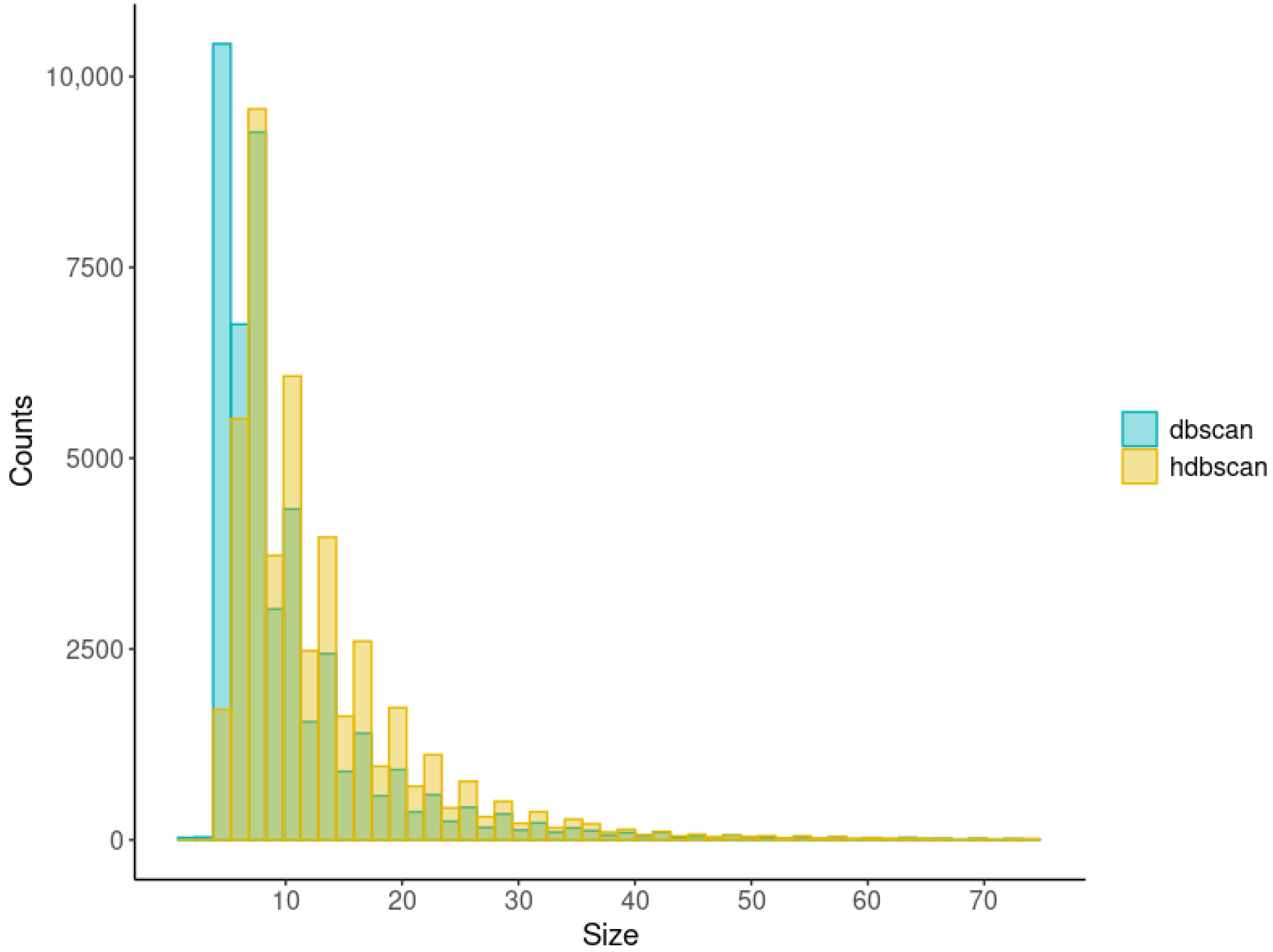
| HDBSCAN | DBSCAN | Parameter |
|---|---|---|
| 605,016 | 475,445 | The number of polymorphisms clusterized |
| 266,609 | 396,180 | The number of polymorphisms not clusterized (noise) |
| 0.69 | 0.55 | The efficiency of clusterization |
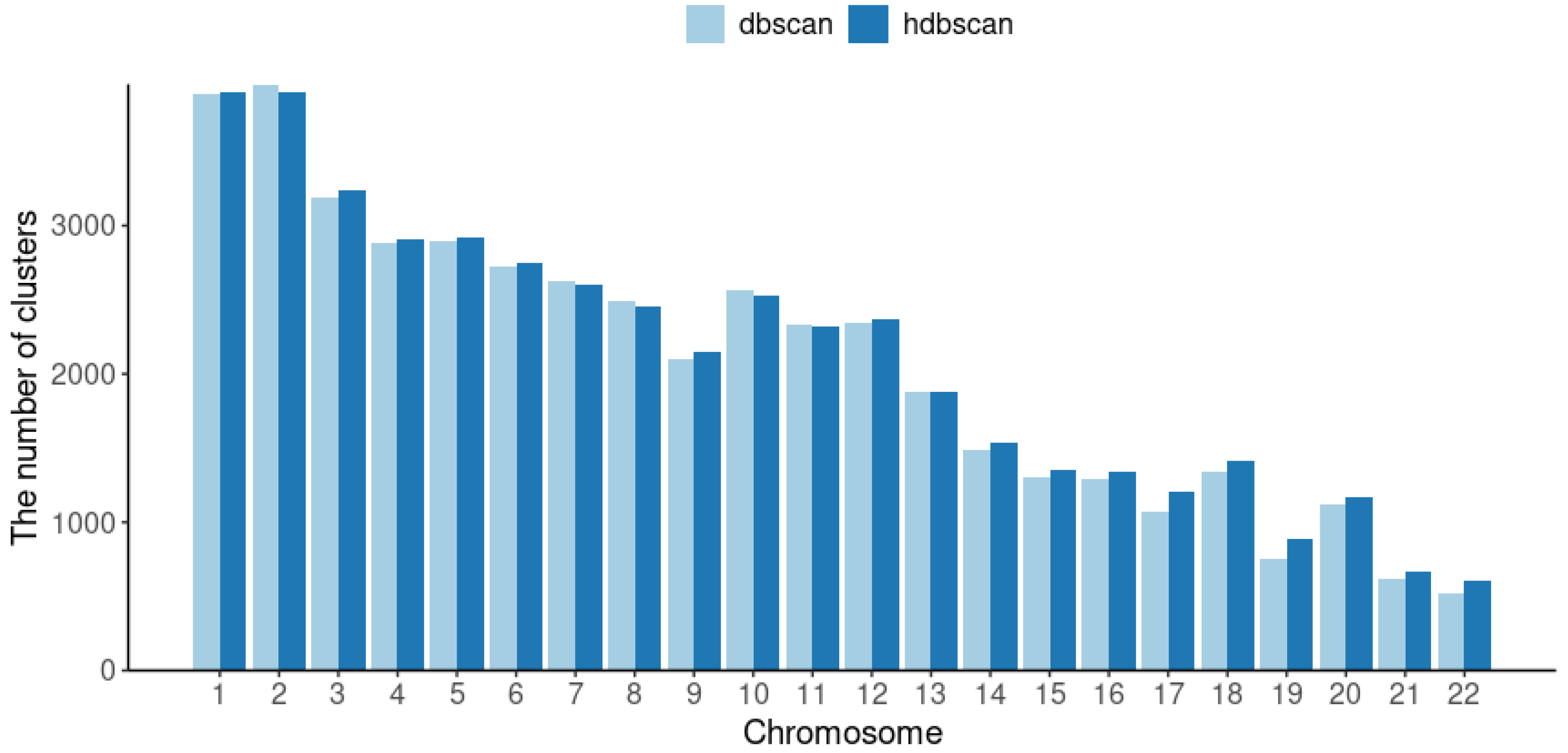
| 46,120 | 45,388 | The number of clusters |
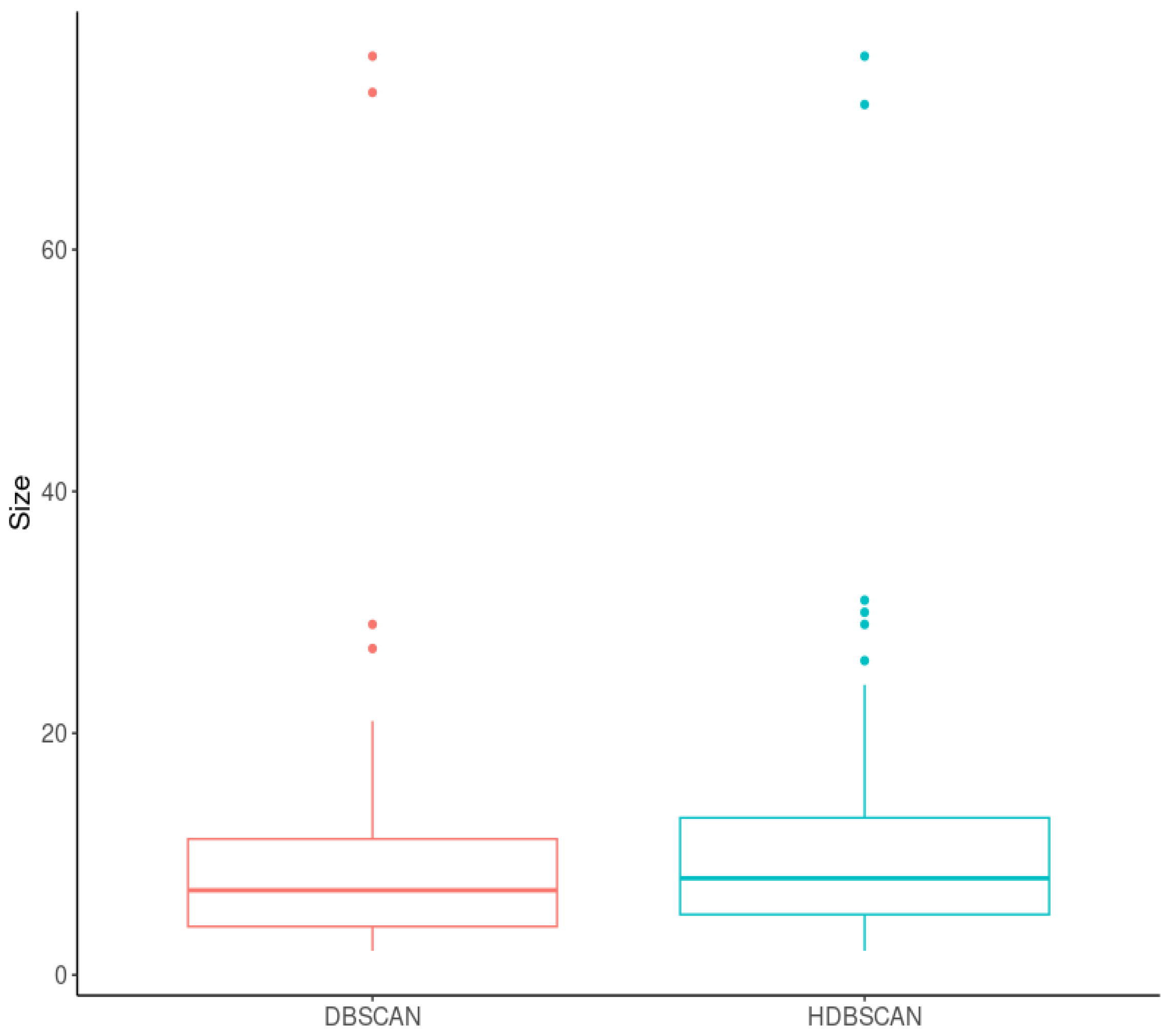
| 5–384 | 1–385 | The minimum and maximum size of clusters |
| 10 | 8 | The median of cluster sizes |
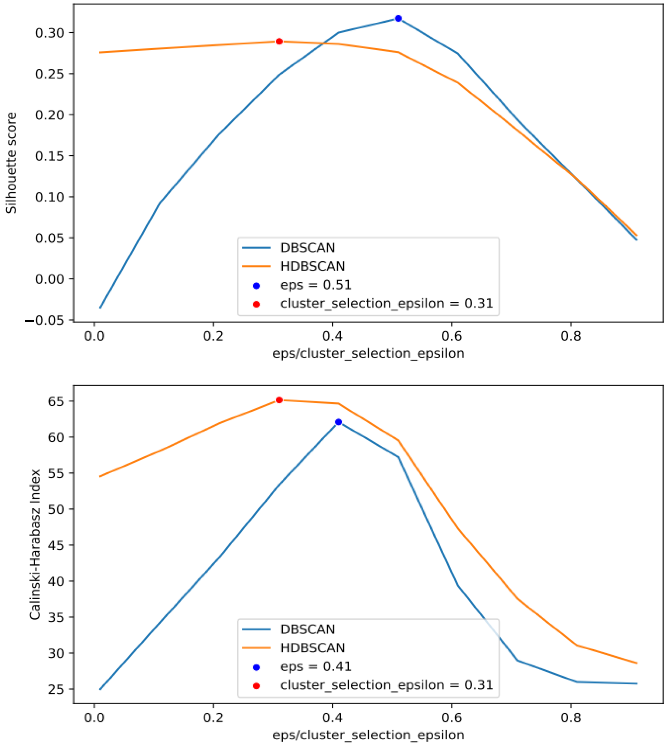
| 0.29 | 0.27 | The mean of Silhouette coefficient |
| 56.4 | 53.2 | The median of Calinski and Harabasz score |
| 44,842 | 41,132 | The number of LD-blocks |
| 79 | 68 | The number of LD-blocks significantly associated with IS |
| 8 | 7 | The median of sizes of LD-blocks associated with IS |
| 892 | 666 | The number of polymorphisms within LD-blocks associated with IS |
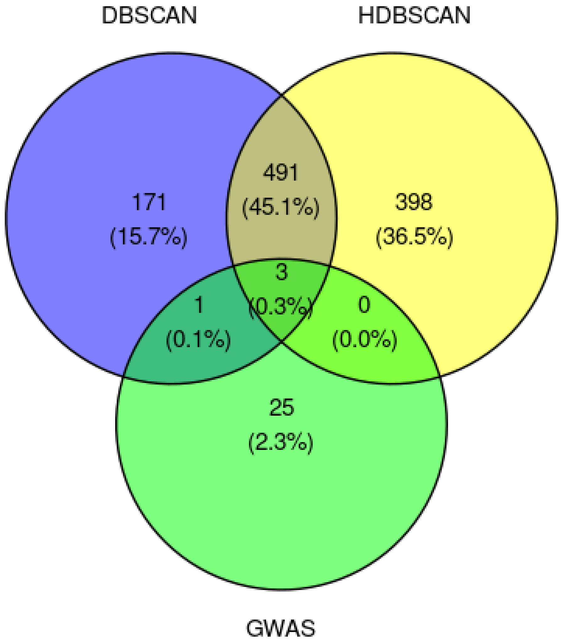
| 122 | 98 | The number of genes and loci associated with IS |
| Cluster-Based GWAS | Classic GWAS | Project |
|---|---|---|
| RUNX1, LHFPL3 | RUNX1 | GWAS Central |
| USF1, CD34, KIF26B, RUNX1 | RUNX1 | DisGeNET |
| – | GPR26 | IDG |
| KIF26B, LHFPL3, RUNX1 | RUNX1 | Monarch Initiative |
| Tested | Downloaded | Project |
|---|---|---|
| 351 | 400 | GWAS Central |
| 1037 | 1159 | DisGeNET |
| 278 | 323 | IDG |
| 116 | 131 | Monarch Initiative |
Disclaimer/Publisher’s Note: The statements, opinions and data contained in all publications are solely those of the individual author(s) and contributor(s) and not of MDPI and/or the editor(s). MDPI and/or the editor(s) disclaim responsibility for any injury to people or property resulting from any ideas, methods, instructions or products referred to in the content. |
© 2023 by the authors. Licensee MDPI, Basel, Switzerland. This article is an open access article distributed under the terms and conditions of the Creative Commons Attribution (CC BY) license (https://creativecommons.org/licenses/by/4.0/).
Share and Cite
Khvorykh, G.V.; Sapozhnikov, N.A.; Limborska, S.A.; Khrunin, A.V. Evaluation of Density-Based Spatial Clustering for Identifying Genomic Loci Associated with Ischemic Stroke in Genome-Wide Data. Int. J. Mol. Sci. 2023, 24, 15355. https://doi.org/10.3390/ijms242015355
Khvorykh GV, Sapozhnikov NA, Limborska SA, Khrunin AV. Evaluation of Density-Based Spatial Clustering for Identifying Genomic Loci Associated with Ischemic Stroke in Genome-Wide Data. International Journal of Molecular Sciences. 2023; 24(20):15355. https://doi.org/10.3390/ijms242015355
Chicago/Turabian StyleKhvorykh, Gennady V., Nikita A. Sapozhnikov, Svetlana A. Limborska, and Andrey V. Khrunin. 2023. "Evaluation of Density-Based Spatial Clustering for Identifying Genomic Loci Associated with Ischemic Stroke in Genome-Wide Data" International Journal of Molecular Sciences 24, no. 20: 15355. https://doi.org/10.3390/ijms242015355
APA StyleKhvorykh, G. V., Sapozhnikov, N. A., Limborska, S. A., & Khrunin, A. V. (2023). Evaluation of Density-Based Spatial Clustering for Identifying Genomic Loci Associated with Ischemic Stroke in Genome-Wide Data. International Journal of Molecular Sciences, 24(20), 15355. https://doi.org/10.3390/ijms242015355