
Tissue Sampling and Homogenization with NIRL Enables Spatially Resolved Cell Layer Specific Proteomic Analysis of the Murine Intestine

 ,
, 
 ,
,  and
and 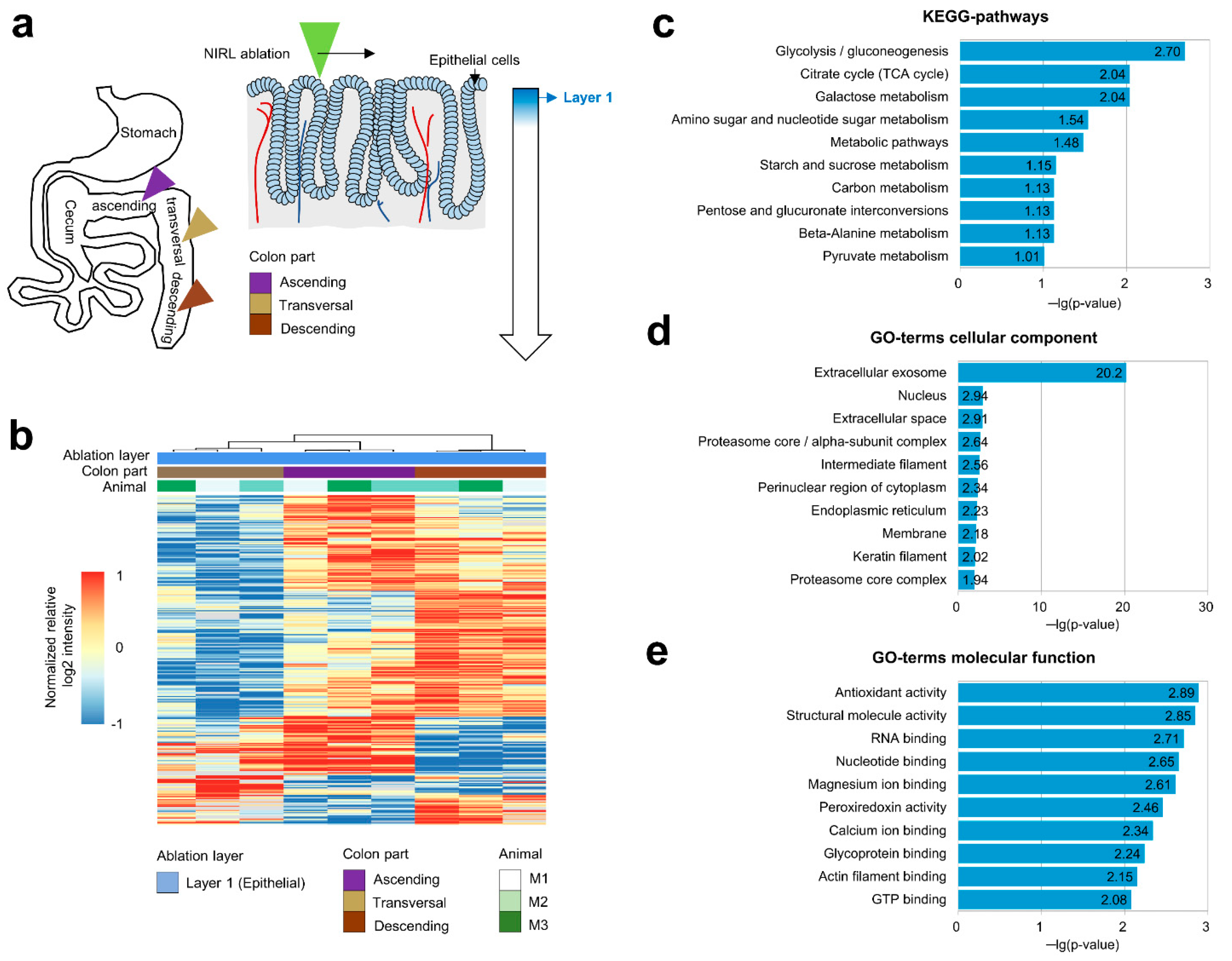
Abstract
:1. Introduction
2. Results
2.1. Analysis of the Proteomes of Different Colon Regions
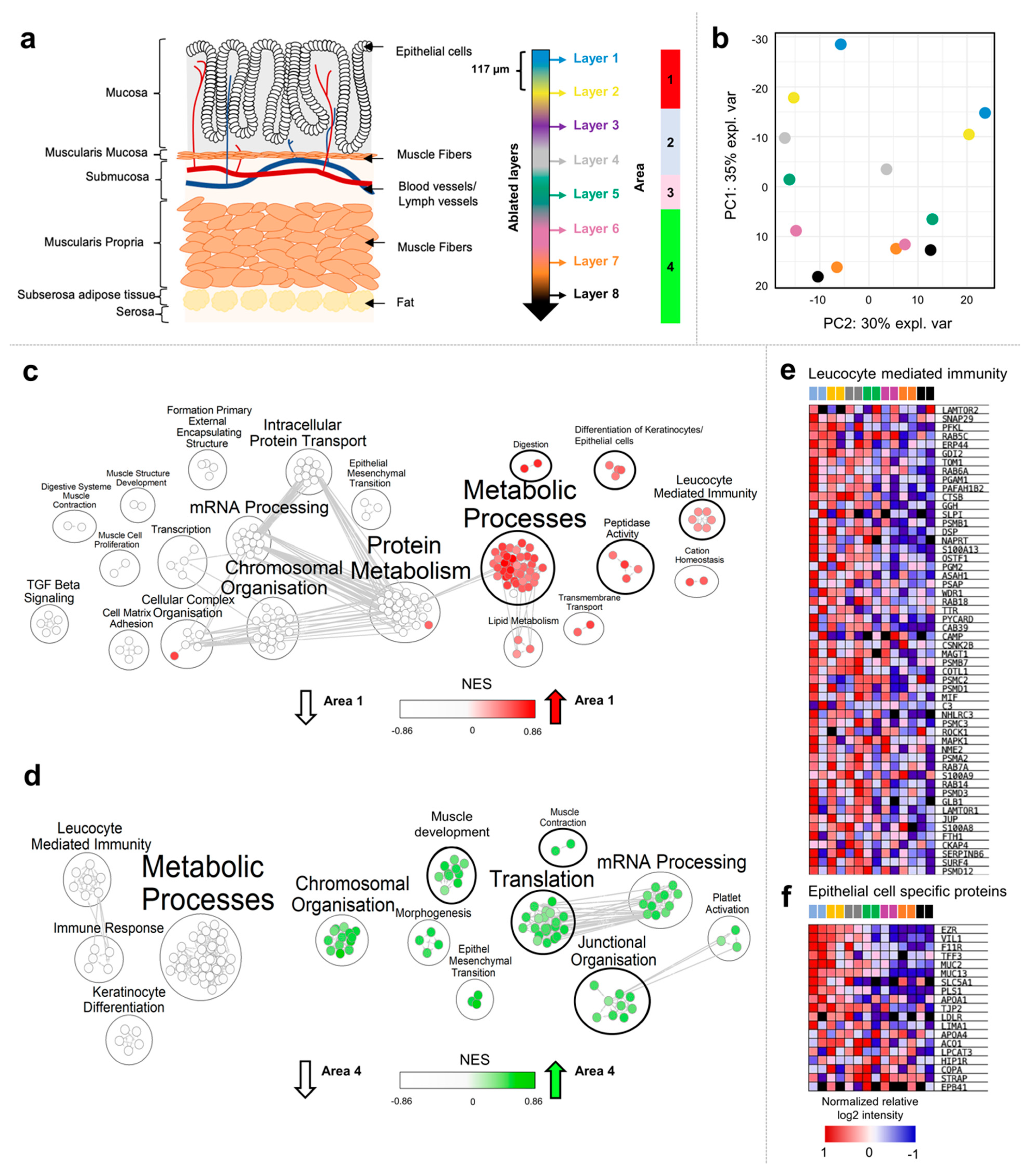
2.2. Analysis of the Proteomes of Consecutive Colon Tissue Layers
3. Discussion
4. Material and Methods
4.1. Animals
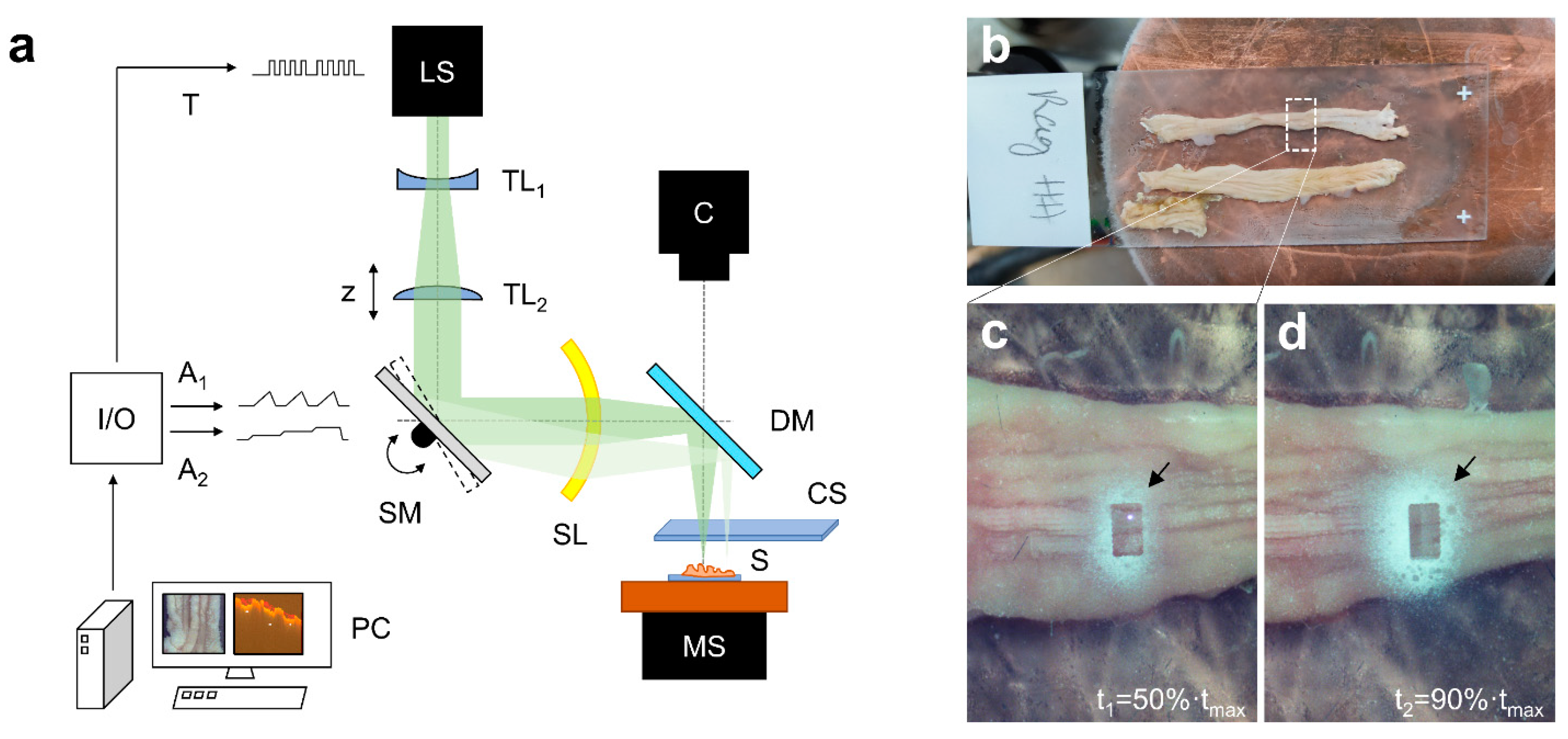
4.2. Ablation Setup
4.3. Tissue Sampling and Collection Procedure
- In the first experiment, one layer was ablated at ascending (A), transversal (B), and descending (C) colon, respectively.
- In the second experiment, 8 consecutive layers were ablated.
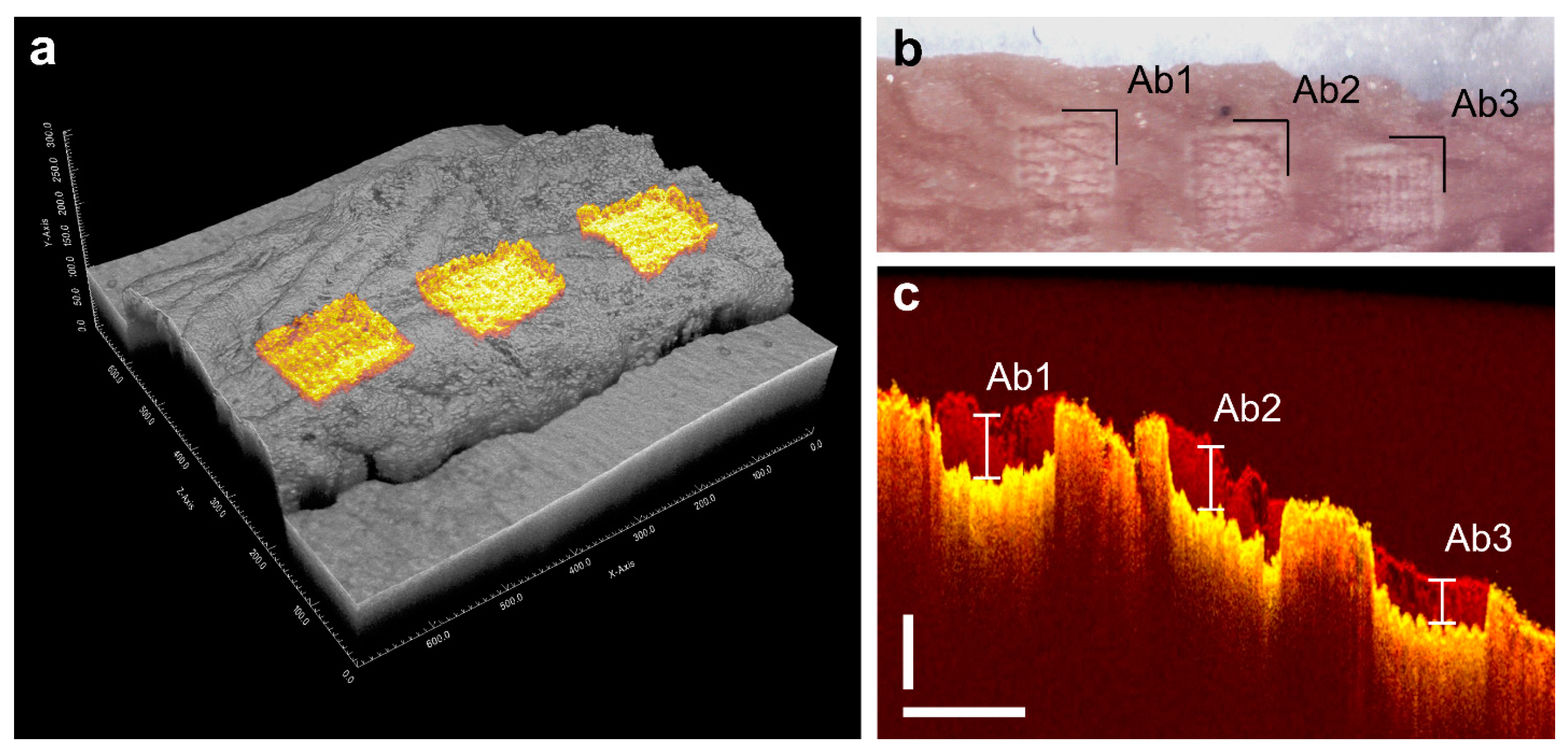
4.4. Determination of Layer Thickness
4.5. Tryptic Digestion of Proteins of the Ablated Tissue Samples
4.6. LC–MS/MS Data Acquisition
4.7. Raw Data Processing
4.8. Data Analysis and Visualization
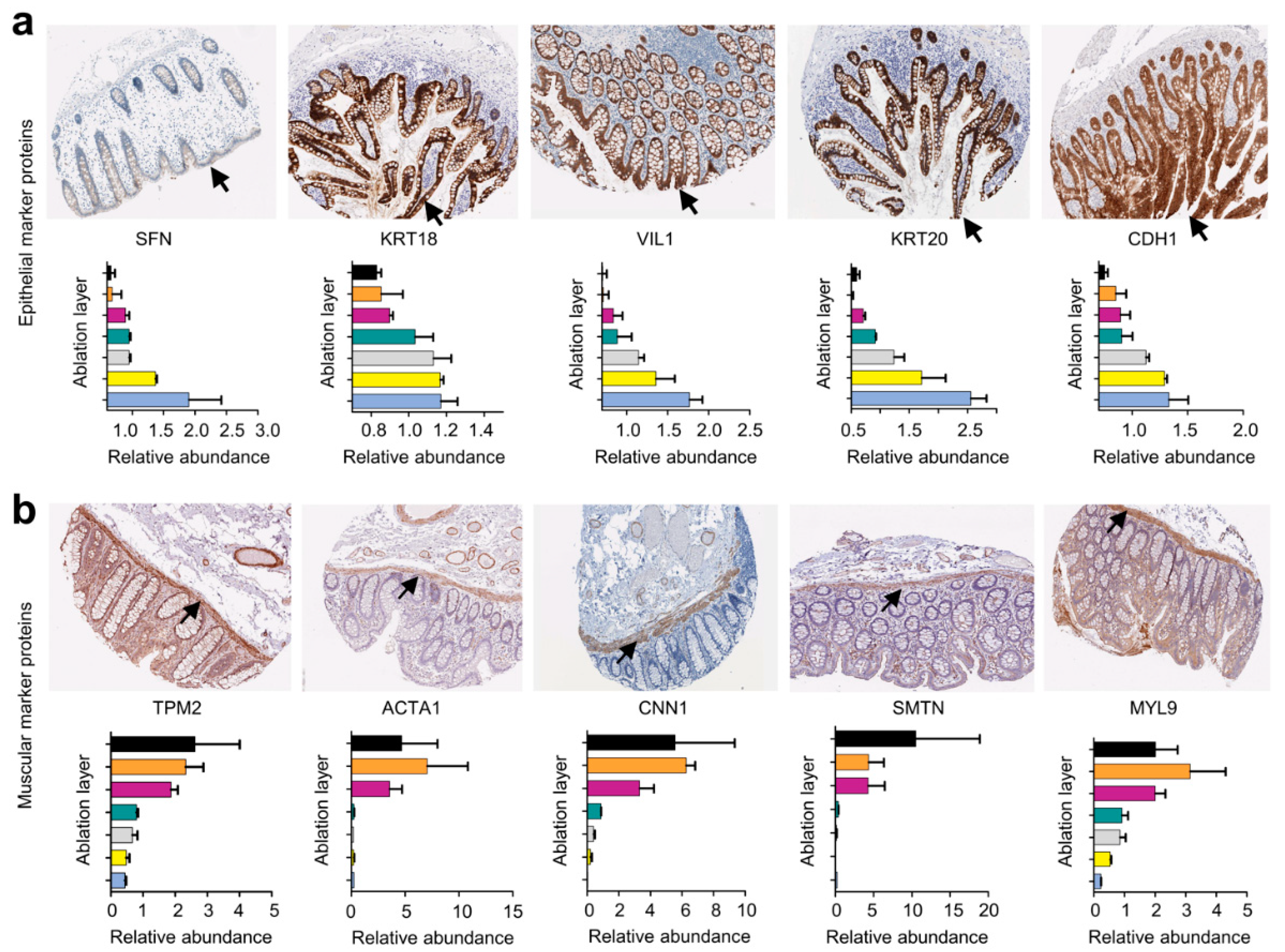
4.9. Histological Staining
- SFN (https://www.proteinatlas.org/ENSG00000175793-SFN/tissue/colon#img), accessed on 29 April 2022;
- KRT18 (https://www.proteinatlas.org/ENSG00000111057-KRT18/tissue/colon#img), accessed on 29 April 2022;
- VIL1 (https://www.proteinatlas.org/ENSG00000127831-VIL1/tissue/colon#img), accessed on 29 April 2022;
- KRT20 (https://www.proteinatlas.org/ENSG00000171431-KRT20/tissue/colon#img), accessed on 29 April 2022;
- CDH1 (https://www.proteinatlas.org/ENSG00000039068-CDH1/tissue/colon#img), accessed on 29 April 2022;
- TPM2 (https://www.proteinatlas.org/ENSG00000198467-TPM2/tissue/colon#img), accessed on 29 April 2022;
- ACTA1 (https://www.proteinatlas.org/ENSG00000143632-ACTA1/tissue/colon#img), accessed on 29 April 2022;
- CNN1 (https://www.proteinatlas.org/ENSG00000130176-CNN1/tissue/colon#img), accessed on 29 April 2022;
- SMTN (https://www.proteinatlas.org/ENSG00000183963-SMTN/tissue/colon#img), accessed on 29 April 2022;
- MYL9 (https://www.proteinatlas.org/ENSG00000101335-MYL9/tissue/colon#img), accessed on 29 April 2022.
Supplementary Materials
Author Contributions
Funding
Institutional Review Board Statement
Informed Consent Statement
Data Availability Statement
Acknowledgments
Conflicts of Interest
References
- Kim, J.; Koo, B.-K.; Knoblich, J.A. Human organoids: Model systems for human biology and medicine. Nat. Rev. Mol. Cell Biol. 2020, 21, 1–14. [Google Scholar] [CrossRef]
- Cañas, B.; Piñeiro, C.; Calvo, E.; López-Ferrer, D.; Gallardo, J.M. Trends in sample preparation for classical and second generation proteomics. J. Chromatogr. A 2007, 1153, 235–258. [Google Scholar] [CrossRef]
- Straube, H.; Witte, C.-P.; Herde, M. Analysis of Nucleosides and Nucleotides in Plants: An Update on Sample Preparation and LC–MS Techniques. Cells 2021, 10, 689. [Google Scholar] [CrossRef]
- Höring, M.; Krautbauer, S.; Hiltl, L.; Babl, V.; Sigruener, A.; Burkhardt, R.; Liebisch, G. Accurate Lipid Quantification of Tissue Homogenates Requires Suitable Sample Concentration, Solvent Composition, and Homogenization Procedure—A Case Study in Murine Liver. Metabolites 2021, 11, 365. [Google Scholar] [CrossRef]
- Menzi, N.; Osinga, R.; Todorov, A.; Schaefer, D.J.; Martin, I.; Scherberich, A. Wet milling of large quantities of human excision adipose tissue for the isolation of stromal vascular fraction cells. Cytotechnology 2018, 70, 807–817. [Google Scholar] [CrossRef]
- Goldberg, S. Mechanical/physical methods of cell disruption and tissue homogenization. Methods Mol. Biol. 2008, 434, 3–22. [Google Scholar]
- Gross, V.; Carlson, G.; Kwan, A.T.; Smejkal, G.; Freeman, E.; Ivanov, A.R.; Lazarev, A. Tissue fractionation by hydrostatic pressure cycling technology: The unified sample preparation technique for systems biology studies. J. Biomol. Tech. JBT 2008, 19, 189–199. [Google Scholar]
- Kehm, R.; Baldensperger, T.; Raupbach, J.; Höhn, A. Protein oxidation-Formation mechanisms, detection and relevance as biomarkers in human diseases. Redox Biol. 2021, 42, 101901. [Google Scholar] [CrossRef]
- Auclair, J.R.; Salisbury, J.; Johnson, J.L.; Petsko, G.A.; Ringe, D.; Bosco, D.A.; Agar, N.Y.R.; Santagata, S.; Durham, H.D.; Agar, J.N. Artifacts to avoid while taking advantage of top-down mass spectrometry based detection of protein S-thiolation. Proteomics 2014, 14, 1152–1157. [Google Scholar] [CrossRef]
- Ji, Y.; Liu, M.; Bachschmid, M.M.; Costello, C.E.; Lin, C. Surfactant-Induced Artifacts during Proteomic Sample Preparation. Anal. Chem. 2015, 87, 5500–5504. [Google Scholar] [CrossRef] [Green Version]
- Bodzoń-Kułakowska, A.; Bierczyńska-Krzysik, A.; Dylag, T.; Drabik, A.; Suder, P.; Noga, M.; Jarzebinska, J.; Silberring, J. Methods for samples preparation in proteomic research. J. Chromatogr. B 2007, 849, 1–31. [Google Scholar] [CrossRef]
- Gil, A.; Siegel, D.; Permentier, H.; Reijngoud, D.-J.; Dekker, F.; Bischoff, R. Stability of energy metabolites-An often overlooked issue in metabolomics studies: A review. Electrophoresis 2015, 36, 2156–2169. [Google Scholar] [CrossRef]
- Svensson, M.; Borén, M.; Sköld, K.; Fälth, M.; Sjögren, B.; Andersson, M.; Svenningsson, P.; Andrén, P.E. Heat Stabilization of the Tissue Proteome: A New Technology for Improved Proteomics. J. Proteome Res. 2009, 8, 974–981. [Google Scholar] [CrossRef] [Green Version]
- Stingl, C.; Söderquist, M.; Karlsson, O.; Borén, M.; Luider, T.M. Uncovering Effects of Ex Vivo Protease Activity during Proteomics and Peptidomics Sample Extraction in Rat Brain Tissue by Oxygen-18 Labeling. J. Proteome Res. 2014, 13, 2807–2817. [Google Scholar] [CrossRef]
- Sköld, K.; Alm, H.; Scholz, B. The Impact of Biosampling Procedures on Molecular Data Interpretation. Mol. Cell. Proteom. 2013, 12, 1489–1501. [Google Scholar] [CrossRef] [Green Version]
- Doll, S.; Dreßen, M.; Geyer, P.E.; Itzhak, D.; Braun, C.; Doppler, S.A.; Meier, F.; Deutsch, M.-A.; Lahm, H.; Lange, R.; et al. Region and cell-type resolved quantitative proteomic map of the human heart. Nat. Commun. 2017, 8, 1–13. [Google Scholar] [CrossRef]
- Mertins, P.; Tang, L.C.; Krug, K.; Clark, D.J.; Gritsenko, M.A.; Chen, L.; Clauser, K.R.; Clauss, T.R.; Shah, P.; Gillette, M.A.; et al. Reproducible workflow for multiplexed deep-scale proteome and phosphoproteome analysis of tumor tissues by liquid chromatography–mass spectrometry. Nat. Protoc. 2018, 13, 1632–1661. [Google Scholar] [CrossRef]
- Emmert-Buck, M.R.; Bonner, R.F.; Smith, P.D.; Chuaqui, R.F.; Zhuang, Z.; Goldstein, S.R.; Weiss, R.A.; Liotta, L.A. Laser capture microdissection. Science 1996, 274, 998–1001. [Google Scholar] [CrossRef]
- Hunt, A.L.; Bateman, N.W.; Barakat, W.; Makohon-Moore, S.; Hood, B.L.; Conrads, K.A.; Zhou, M.; Calvert, V.; Pierobon, M.; Loffredo, J.; et al. Extensive three-dimensional intratumor proteomic heterogeneity revealed by multiregion sampling in high-grade serous ovarian tumor specimens. iScience 2021, 24, 102757. [Google Scholar] [CrossRef]
- Magdeldin, S.; Yamamoto, T. Toward deciphering proteomes of formalin-fixed paraffin-embedded (FFPE) tissues. Proteomics 2012, 12, 1045–1058. [Google Scholar] [CrossRef]
- Kwiatkowski, M.; Wurlitzer, M.; Omidi, M.; Ren, L.; Kruber, S.; Nimer, R.; Robertson, W.D.; Horst, P.-D.D.A.; Miller, R.J.D.; Schlüter, H. Ultrafast Extraction of Proteins from Tissues Using Desorption by Impulsive Vibrational Excitation. Angew. Chem. Int. Ed. 2014, 54, 285–288. [Google Scholar] [CrossRef]
- Kwiatkowski, M.; Wurlitzer, M.; Krutilin, A.; Kiani, P.; Nimer, R.; Omidi, M.; Mannaa, A.; Bussmann, T.; Bartkowiak, K.; Kruber, S.; et al. Homogenization of tissues via picosecond-infrared laser (PIRL) ablation: Giving a closer view on the in-vivo composition of protein species as compared to mechanical homogenization. J. Proteom. 2016, 134, 193–202. [Google Scholar] [CrossRef]
- Krutilin, A.; Maier, S.; Schuster, R.; Kruber, S.; Kwiatkowski, M.; Robertson, W.D.; Hansen, N.-O.; Miller, R.J.D.; Schlüter, H. Sampling of Tissues with Laser Ablation for Proteomics: Comparison of Picosecond Infrared Laser and Microsecond Infrared Laser. J. Proteome Res. 2019, 18, 1451–1457. [Google Scholar] [CrossRef]
- Dong, C.; Richardson, L.T.; Solouki, T.; Murray, K.K. Infrared Laser Ablation Microsampling with a Reflective Objective. J. Am. Soc. Mass Spectrom. 2022, 33, 463–470. [Google Scholar] [CrossRef]
- Donnarumma, F.; Murray, K.K. Laser ablation sample transfer for localized LC-MS/MS proteomic analysis of tissue. J. Mass Spectrom. 2016, 51, 261–268. [Google Scholar] [CrossRef]
- Hahn, J.; Moritz, M.; Voß, H.; Pelczar, P.; Huber, S.; Schlüter, H. Tissue Sampling and Homogenization in the Sub-Microliter Scale with a Nanosecond Infrared Laser (NIRL) for Mass Spectrometric Proteomics. Int. J. Mol. Sci. 2021, 22, 10833. [Google Scholar] [CrossRef]
- Uhlén, M.; Fagerberg, L.; Hallström, B.M.; Lindskog, C.; Oksvold, P.; Mardinoglu, A.; Sivertsson, Å.; Kampf, C.; Sjöstedt, E.; Asplund, A.; et al. Tissue-based map of the human proteome. Science 2015, 347, 6220. [Google Scholar] [CrossRef]
- Johnson, L.R. Regulation of gastrointestinal mucosal growth. Physiol. Rev. 1988, 68, 456–502. [Google Scholar] [CrossRef]
- Baxter, B.A.; Parker, K.D.; Nosler, M.J.; Rao, S.; Craig, R.; Seiler, C.; Ryan, E.P. Metabolite profile comparisons between ascending and descending colon tissue in healthy adults. World J. Gastroenterol. 2020, 26, 335–352. [Google Scholar] [CrossRef]
- Jensen, S.R.; Schoof, E.M.; Wheeler, S.E.; Hvid, H.; Ahnfelt-Rønne, J.; Hansen, B.F.; Nishimura, E.; Olsen, G.S.; Kislinger, T.; Brubaker, P.L. Quantitative Proteomics of Intestinal Mucosa From Male Mice Lacking Intestinal Epithelial Insulin Receptors. Endocrinology 2017, 158, 2470–2485. [Google Scholar] [CrossRef] [Green Version]
- Lyons, J.; Ghazi, P.C.; Starchenko, A.; Tovaglieri, A.; Baldwin, K.R.; Poulin, E.J.; Gierut, J.J.; Genetti, C.; Yajnik, V.; Breault, D.T.; et al. The colonic epithelium plays an active role in promoting colitis by shaping the tissue cytokine profile. PLOS Biol. 2018, 16, e2002417. [Google Scholar] [CrossRef] [Green Version]
- Schindelin, J.; Arganda-Carreras, I.; Frise, E.; Kaynig, V.; Longair, M.; Pietzsch, T.; Preibisch, S.; Rueden, C.; Saalfeld, S.; Schmid, B.; et al. Fiji: An open-source platform for biological-image analysis. Nat. Methods 2012, 9, 676–682. [Google Scholar] [CrossRef] [Green Version]
- Fernandez, R.; Moisy, C. Fijiyama: A registration tool for 3D multimodal time-lapse imaging. Bioinformatics 2020, 37, 1482–1484. [Google Scholar] [CrossRef]
- Yushkevich, P.A.; Piven, J.; Hazlett, H.C.; Smith, R.G.; Ho, S.; Gee, J.C.; Gerig, G. User-guided 3D active contour segmentation of anatomical structures: Significantly improved efficiency and reliability. NeuroImage 2006, 31, 1116–1128. [Google Scholar] [CrossRef] [Green Version]
- Rohart, F.; Gautier, B.; Singh, A.; Lê Cao, K.-A. mixOmics: An R package for ‘omics feature selection and multiple data integration. PLoS Comput. Biol. 2017, 13, e1005752. [Google Scholar] [CrossRef] [Green Version]
- Wilkerson, M.D.; Hayes, D.N. ConsensusClusterPlus: A class discovery tool with confidence assessments and item tracking. Bioinformatics 2010, 26, 1572–1573. [Google Scholar] [CrossRef] [Green Version]
- Fabregat, A.; Jupe, S.; Matthews, L.; Sidiropoulos, K.; Gillespie, M.; Garapati, P.; Haw, R.; Jassal, B.; Korninger, F.; May, B.; et al. The Reactome Pathway Knowledgebase. Nucleic Acids Res. 2018, 46, D649–D655. [Google Scholar] [CrossRef] [PubMed]
- Subramanian, A.; Tamayo, P.; Mootha, V.K.; Mukherjee, S.; Ebert, B.L.; Gillette, M.A.; Paulovich, A.; Pomeroy, S.L.; Golub, T.R.; Lander, E.S.; et al. Gene set enrichment analysis: A knowledge-based approach for interpreting genome-wide expression profiles. Proc. Natl. Acad. Sci. USA 2005, 102, 15545–15550. [Google Scholar] [CrossRef] [Green Version]
- Shannon, P.; Markiel, A.; Ozier, O.; Baliga, N.S.; Wang, J.T.; Ramage, D.; Amin, N.; Schwikowski, B.; Ideker, T. Cytoscape: A software environment for integrated models of Biomolecular Interaction Networks. Genome Res. 2003, 13, 2498–2504. [Google Scholar] [CrossRef]
- Merico, D.; Isserlin, R.; Stueker, O.; Emili, A.; Bader, G.D. Enrichment Map: A Network-Based Method for Gene-Set Enrichment Visualization and Interpretation. PLoS ONE 2010, 5, e13984. [Google Scholar] [CrossRef]
- Millán, P.P.; Kucera, M.; Isserlin, R.; Arkhangorodsky, A.; Bader, G.D. Referee report. For: AutoAnnotate: A Cytoscape app for summarizing networks with semantic annotations [version 1; referees: 1 approved]. Natl. Cent. Biotechnol. Inf. 2016, 5, 1717. [Google Scholar] [CrossRef]
- Liberzon, A.; Birger, C.; Thorvaldsdóttir, H.; Ghandi, M.; Mesirov, J.P.; Tamayo, P. The Molecular Signatures Database Hallmark Gene Set Collection. Cell Syst. 2015, 1, 417–425. [Google Scholar] [CrossRef] [PubMed] [Green Version]
- Dennis, G.; Sherman, B.T.; Hosack, D.A.; Yang, J.; Gao, W.; Lane, H.C.; Lempicki, R.A. DAVID: Database for Annotation, Visualization, and Integrated Discovery. Genome Biol. 2003, 4, 5. [Google Scholar] [CrossRef] [Green Version]
- Harris, M.A. The Gene Oncology (GO) database and informatics resource. Nucleic Acids Res. 2004, 32, 258–261. [Google Scholar]


Publisher’s Note: MDPI stays neutral with regard to jurisdictional claims in published maps and institutional affiliations. |
© 2022 by the authors. Licensee MDPI, Basel, Switzerland. This article is an open access article distributed under the terms and conditions of the Creative Commons Attribution (CC BY) license (https://creativecommons.org/licenses/by/4.0/).
Share and Cite
Voß, H.; Moritz, M.; Pelczar, P.; Gagliani, N.; Huber, S.; Nippert, V.; Schlüter, H.; Hahn, J. Tissue Sampling and Homogenization with NIRL Enables Spatially Resolved Cell Layer Specific Proteomic Analysis of the Murine Intestine. Int. J. Mol. Sci. 2022, 23, 6132. https://doi.org/10.3390/ijms23116132
Voß H, Moritz M, Pelczar P, Gagliani N, Huber S, Nippert V, Schlüter H, Hahn J. Tissue Sampling and Homogenization with NIRL Enables Spatially Resolved Cell Layer Specific Proteomic Analysis of the Murine Intestine. International Journal of Molecular Sciences. 2022; 23(11):6132. https://doi.org/10.3390/ijms23116132
Chicago/Turabian StyleVoß, Hannah, Manuela Moritz, Penelope Pelczar, Nicola Gagliani, Samuel Huber, Vivien Nippert, Hartmut Schlüter, and Jan Hahn. 2022. "Tissue Sampling and Homogenization with NIRL Enables Spatially Resolved Cell Layer Specific Proteomic Analysis of the Murine Intestine" International Journal of Molecular Sciences 23, no. 11: 6132. https://doi.org/10.3390/ijms23116132
APA StyleVoß, H., Moritz, M., Pelczar, P., Gagliani, N., Huber, S., Nippert, V., Schlüter, H., & Hahn, J. (2022). Tissue Sampling and Homogenization with NIRL Enables Spatially Resolved Cell Layer Specific Proteomic Analysis of the Murine Intestine. International Journal of Molecular Sciences, 23(11), 6132. https://doi.org/10.3390/ijms23116132