Application of the XBoost Regressor for an A Priori Prediction of UAV Image Quality

Abstract

In general, the quality of imagery from Unmanned Aerial Vehicles (UAVs) is evaluated after the flight, and then a decision is made on the further value and use of the acquired data. In this paper, an a priori (preflight) image quality prediction methodology is proposed to estimate the preflight image quality and to avoid unfavourable flights, which is extremely important from a time and cost management point of view. The XBoost Regressor model and cross-validation were used for machine learning of the model and image quality prediction. The model was learned on a rich database of real-world images acquired from UAVs under conditions varying in both sensor type, UAV type, exposure parameters, weather, topography, and land cover. Radiometric quality indices (SNR, Entropy, PIQE, NIQE, BRISQUE, and NRPBM) were calculated for each image to train and test the model and to assess the accuracy of image quality prediction. Different variants of preflight parameter knowledge were considered in the study. The proposed methodology offers the possibility of predicting image quality with high accuracy. The correlation coefficient between the actual and predicted image quality, depending on the number of parameters known a priori, ranged from 0.90 to 0.96. The methodology was designed for data acquired from a UAV. Similar prediction accuracy is expected for other low-altitude or close-range photogrammetric data.

1. Introduction

Currently, a significant amount of information is obtained by interpreting images taken from various altitudes, from close range photogrammetry, through UAV (Unmanned Aerial Vehicle) images, to satellite imagery. Obviously, the better the quality of the image, the more information can be obtained from it. If the image is blurred, out of focus, or noised, its interpretation will be difficult or even impossible. Therefore, acquiring images of the highest possible quality, as well as ways to correct these images to eliminate distortions and improve radiometric quality, is an important and topical issue. Since satellite images began to be acquired, techniques for their correction have also been developed [1,2,3,4,5]. Currently, there are many algorithms dedicated to this task. However, the correction of images acquired from a low altitude is a relatively new topic. Various studies are still underway to find the right methods to improve the quality of UAV images [1,6,7]. The effectiveness of these methods for images acquired under widely varying conditions is still not explicitly confirmed. Therefore, it remains an important task to design a photogrammetric flight in such a way as to guarantee the best possible image quality. So far, the operator of an unmanned platform has intuitively determined the right conditions for the flight. The quality of the images, on the other hand, is only assessed after their acquisition. 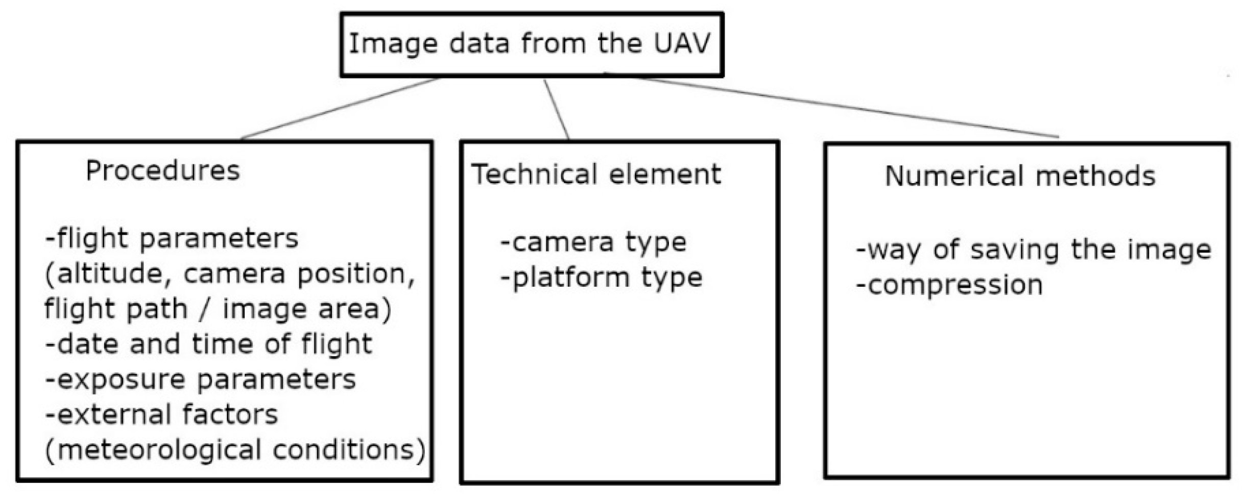The radiometric quality of the images is affected by many factors such as exposure parameters and sensor properties, flight parameters, and external conditions [8]. 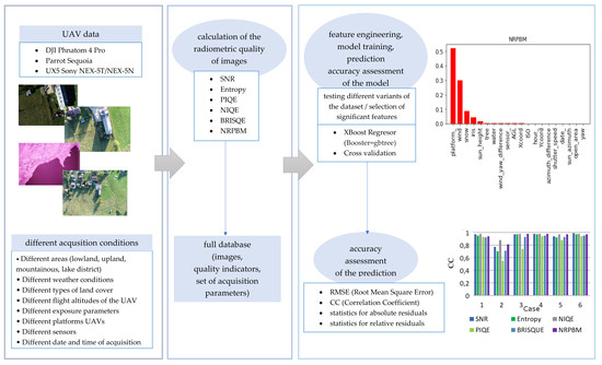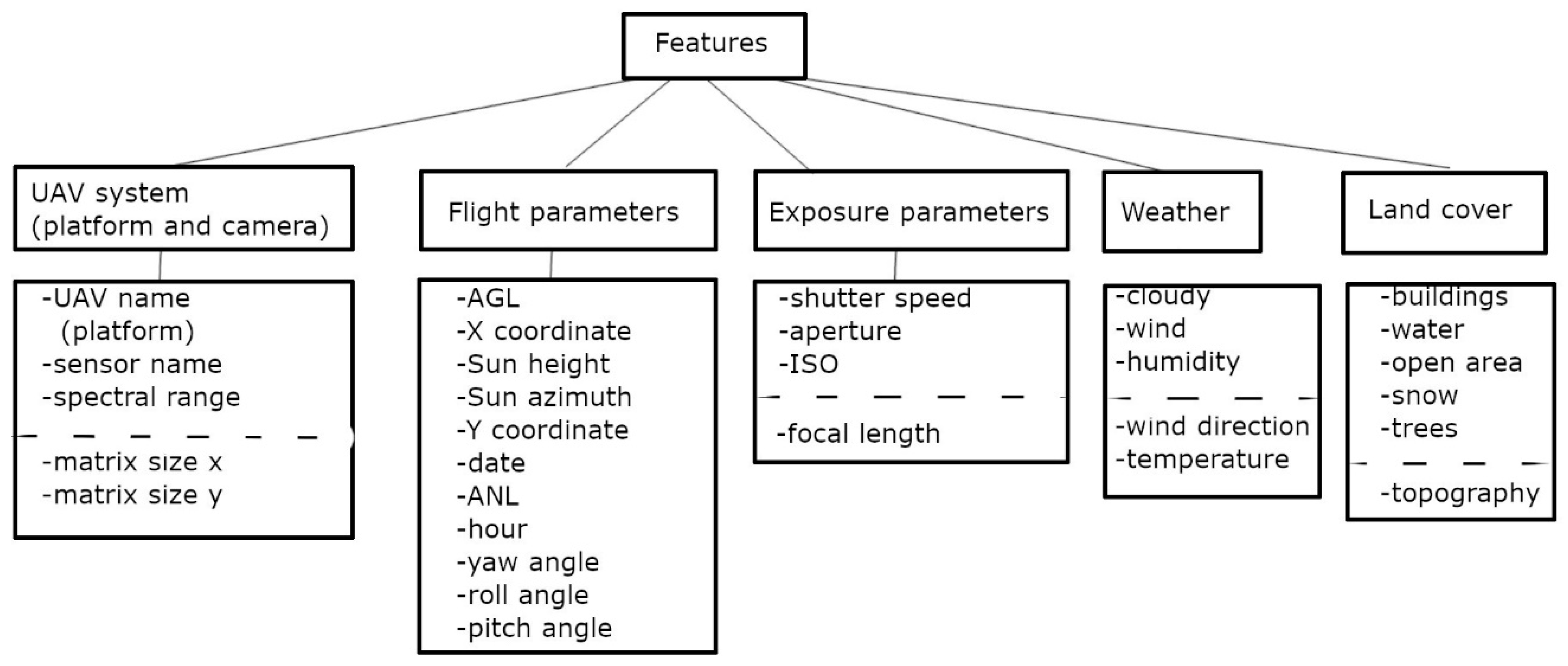There are three groups of factors that influence the quality of images and the whole photogrammetric process: procedures, technical elements, and numerical methods [9]. Procedures refer to parameters related to imagery data collection. Technical elements are all technical devices and their quality. Numerical methods are the capabilities and properties of algorithms and mathematical methods used for data processing in the photogrammetric process. Based on the above, the factors that affect the quality of images acquired by UAVs can be grouped, as shown in Figure 1.

The quality of imagery data acquired by UAVs is primarily influenced by procedural factors, which can include flight parameters, date and time of image acquisition, exposure parameters, and external factors. Among the flight parameters, the flight altitude, camera position, and flight location (imaged terrain) are of particular importance. The altitude affects the spatial resolution of the image. In addition, at a higher altitude, stronger winds may occur and a stronger haze of the image at high humidity is noticeable, resulting in a lower radiometric quality of the image [3].

Moreover, the quality of any photograph is affected by the exposure parameters. The ISO parameter determines the sensitivity of the sensor to light, and is one of the main factors responsible for the noise in the image [10,11]. Exposure time and aperture determine how much light reaches the sensor. A particular challenge is the selection of the exposure parameters for images taken in low light conditions. This problem occurs in practice quite often when there is a need to perform a flight with an unmanned platform early in the morning, at dusk, or during poor weather conditions. If the camera is set to a long exposure time, the image is blurred due to camera movement. On the other hand, the image is dark and noisy if it is taken with a short exposure time but with high camera gain [11].

In addition, flight parameters and external factors such as weather and lighting significantly affect the quality of the image. The date and time of capture are important, as they are closely related to the position of the sun, its azimuth, and height above the horizon. This firstly influences the amount of sunlight on the scene and secondly the uniformity of the illumination. The azimuth of the sun, in conjunction with the tilt and twist angles of the platform, can cause uneven illumination of the scene and therefore nonuniform image brightness [7,12]. Uneven illumination (caused by platform tilt or shadow) causes some pixels to receive too little light. The image is locally underexposed. Then, the image quality in such places is lower than in places with proper illumination. The graininess is increased, especially noticeable in shaded areas. This reduces the legibility of the image, the information potential, and the quality of the phorogrammetric products [3,13]. The wind is a very important factor as it affects the speed. The wind influences the tilt of the platform and, therefore, sometimes (depending on the type of platform) can cause a change in the tilt and twist angles of the camera. This factor is particularly important for platforms without a gimbal stabilising the camera. Light airframes are particularly sensitive to the influence of wind.

Image quality is also closely dependent on technical factors, so it depends on the properties of the imaging system. The type of sensor affects the level of image noise [14]. The type of lens affects the distortion [15]. Platform vibrations (often caused by poor vibroisolation and lack of stabilizing gimbals) can cause image blur and a jello effect [16,17,18]. Furthermore, the radiometric quality of images is affected by the sensitivity range of the sensor. Images recorded in the infrared range are susceptible to noise [19,20]. Above all, thermal infrared imaging sensors are characterised by high noise [21].

The last group of factors influencing the quality of an image concerns numerical factors. This group of factors is especially important when analysis is performed on post-processed images or even finished photogrammetric products. Each processing step affects the final image quality. When assessing the quality of unprocessed UAV images, the way they are stored and compressed may be important.

The quality of UAV images is crucial for many analyses. Radiometric quality primarily affects remote sensing analyses such as classification and change detection [22,23]. Furthermore, correct radiometric quality is important especially in cases where images are acquired in adverse weather conditions. In this situation, their poor radiometric quality often results in an incorrect image block adjustment or makes such an adjustment impossible [24]. In recent years, various methods have been developed to improve image quality, especially using neural networks. In photogrammetric studies, the blurring of images is a major difficulty. One of the effective solutions to remove blurring, which significantly increases the final geometric quality of photogrammetric products, is the use of generative adversarial networks (GANs) [25,26] or a discriminative model [27]. To improve the spatial quality of the image, techniques based on super resolution are often used, which are now intensively developed through the use of deep learning [28,29]. An enhanced superresolution generative adversarial network (ESRGAN) has been proposed to predict the degradation or loss of spatial information in a set of RGB images with hyperspatial resolution [30]. Image dehazing is a common problem in UAV photogrammetry. Moreover, this issue recently has effective solutions based on neural networks, such as: a multiscale deep neural network for single image dehazing by learning the mapping between hazy images and their transmission maps [31]; a mix of RMAM, group convolution, depth-wise convolution, and point-wise convolution [32]; and a combination of an end-to-end Haze Concentration Adaptive Network (HCAN), including a pyramid feature extractor (PFE), a feature enhancement module (FEM), and a multiscale feature attention module (MSFAM) [33].

Image quality is generally assessed a posteriori using special indicators [3,16,25,26] Far fewer studies have addressed image quality prediction. The solution described in [34] proposes an algorithm adapted to all images, which can also be applied to UAV images. However, it considers the question of assessing image quality based on the study of noise (named errors there). An error (noise) map is created for the test images and then predicted for the remaining images. The quality prediction thus takes place in some internal system of the image. Distortions are predicted already in the image itself [34,35]. In this manuscript, a solution is proposed where image quality is assessed a priori, based on several previously known parameters and their relationship to image quality assessment indicators. This research aimed to predict the image quality of a UAV image based on a set of external factors known before the flight was performed. Until now, the UAV platform operator has intuitively determined the conditions appropriate for flight execution. The quality of the images, on the other hand, is only assessed after they are acquired. Therefore, some flights have turned out to be unusable, because the images were of too low quality.

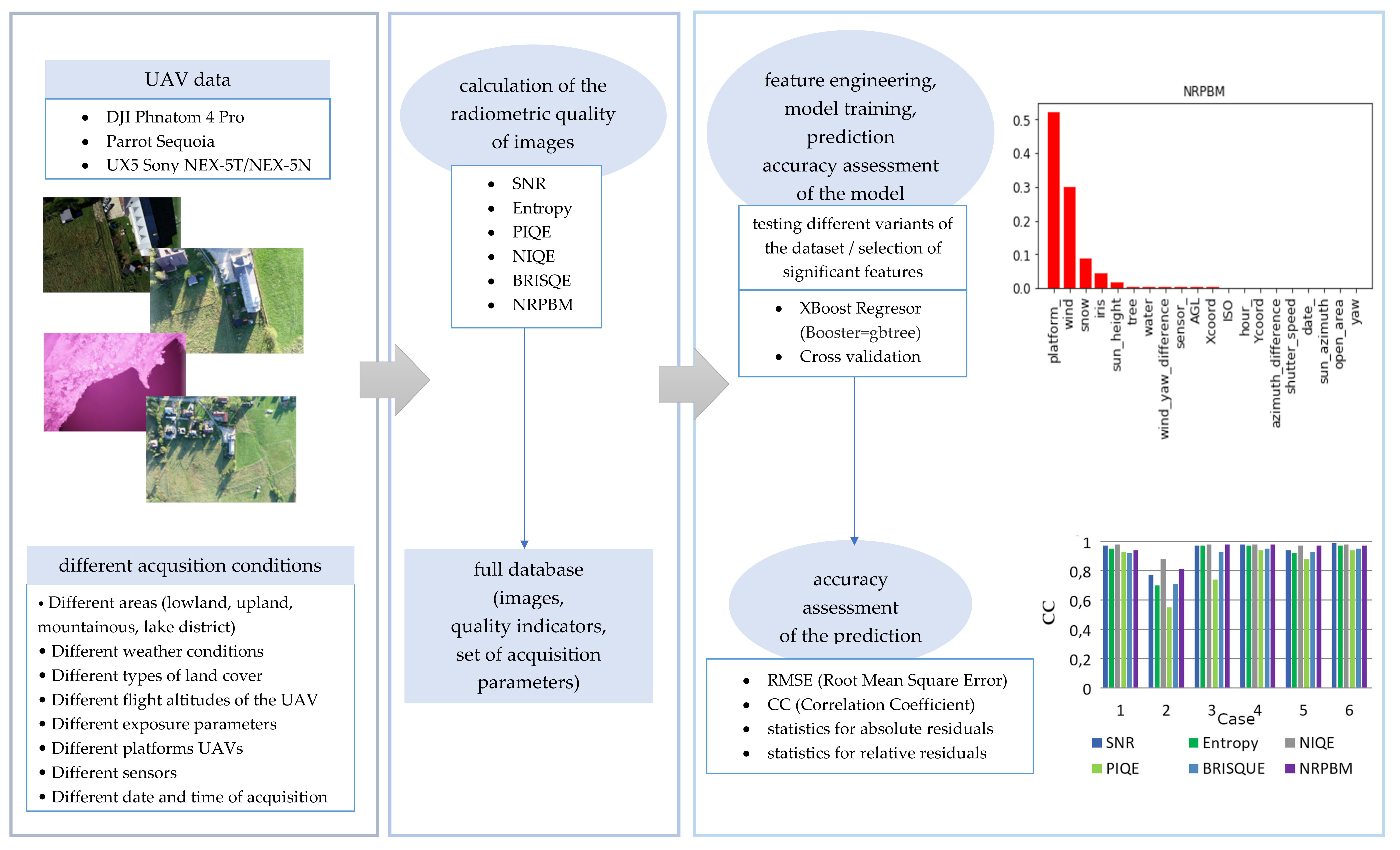
The method proposed in this article will make it possible to estimate the quality of the photos before the flight and to avoid unfavourable flights, which is extremely important from the point of view of time and cost management. This manuscript presents the possibility of using the XBoost Regressor for a priori prediction of UAV image quality. Image datasets from different UAVs were acquired, all under a variety of conditions. For each image, values of metrics describing its radiometric quality were added to the acquired database. Then, based on these datasets, the model was trained to predict image quality based on a series of parameters known prior to flight. Several variants of levels of knowledge of the factors affecting image quality were considered in the study. For each variant, model accuracy, and prediction accuracy were assessed. The proposed methodology is described in detail in Section 4 (Methodology). The results of the research are presented in Section 5 (Results).

2. Overview of Image Quality Assessment Methods

A key step in the prediction of image quality is the selection of a method to assess this quality. Methods for assessing radiometric image quality are divided into quantitative and qualitative. Qualitative methods are most often based on visual analysis. For years, they have been recognised as the most reliable, as no algorithms can fully replace the human eye. However, these methods are subjective, lengthy, and expensive [36]. Much more popular is the use of quantitative methods, which involve the determination of special metrics dedicated to the assessment of radiometric quality. These methods can be divided into relative and absolute methods. Relative methods require a reference to an ideal image, one without radiometric distortions. These include MSE (Mean Square Error), RMSE (Root Mean Square Error), CC (Correlation Coefficient), SSIM (Structural Similarity Index), MSSIM (Multi-Scale Structural Similarity Index) [37], PSNR (Peak Signal-to-Noise Ratio), and SNR (Signal-to-Noise Ratio). MSE and RMSE are simple indices that are based on calculating the differences between the compared images. The lower the value, the higher the image quality. CC is based on a similarity analysis between two images. PSNR measures the ratio of the maximum power of a signal to the power of noise interfering with that signal, where the original image is considered to be the signal. Analogously, two images can be compared using SNR. PSNR and SNR are then considered as relative assessment methods. In general, these methods are used when an original image of high radiometric quality is available or when such an image can be simulated. The SSIM algorithm, on the other hand, compares two images in terms of their luminance, contour, and structure. The structure of the objects in a scene is independent of local luminance and contrast. Therefore, to extract the structural information, we should separate the effect of illumination. In this algorithm, structural information in an image is defined as those traits that represent the structure of objects in that image, independent of the local luminance and contrast [38,39]. MSSIM is based on similar assumptions, but due to its multiscale nature, it provides a more flexible metric [37].

Relative methods are very well suited for testing the effectiveness of different image processing techniques, where the image before and after processing is compared for quality assessment. The results of such an assessment are reliable, but they are dependent on the quality of the original image. Relative methods provide the basis for more complex solutions, such as the use of watermarking to assess the quality of compressed images [40]. This solution is based on the PSNR index. Another method is based on comparing the structural information extracted from the distorted image and the original image. This method uses reduced references containing perceptual structural information [41]. Another proposal is based on comparing the local variance distribution of two images and on the image structure [42].

Absolute methods do not require a reference image. They rely on the analysis of properties (generally statistical parameters) of the image in question. The most popular absolute methods include Entropy, PIQE (Perception-based Image Quality Evaluator), NIQE (Natural Image Quality Evaluator), BRISQUE (Blind/Referenceless Image Spatial Quality Evaluator). PIQE involves extracting local features to predict quality. Quality is evaluated only from perceptually relevant spatial regions, but at the same time, PIQE does not require supervised learning [43]. NIQE and BRISQUE indicators are based on a simple and successful space domain natural scene statistic model. NIQE uses only measurable deviations from statistical regularities observed in natural images, without training on distorted images evaluated by humans, or even without any exposure to distorted images [44]. BRISQUE is a model also trained on distorted images. As a result, BRISQUE is more sensitive to the distortions present in the images and its performance is limited to the distortions on which it was trained. BRISQUE does not calculate distortion characteristics such as blurring or blocking but, instead, uses scene statistics of locally normalised luminance coefficients, leading to an overall quality measurement. BRISQUE has very low computational complexity, making it well suited for realtime applications, and its results are more reliable compared to classical SNR [44,45]. In [46], a No-Reference Perceptual Blur Metric (NRPBM) was proposed for image blur evaluation, which is based on distinguishing different levels of blur perceivable in the same image. The NRPBM takes values ranging from 0 to 1, which characterise the best and the worst image quality in terms of blur, respectively. Additionally, the SNR can be used as an absolute evaluation method when we do not refer to a reference image but only study the statistics of the analysed image. On the other hand, a reference-free image quality assessment algorithm based on a general regression neural network (GRNN) uses the mean value of the phase congruency image, the entropy of phase congruency image, the entropy of the distorted image, and the gradient of the distorted image. Image quality assessment is achieved by approximating the functional relationship between these features and subjective mean opinion scores using GRNN [47]. Another relatively new solution uses a convolutional neural network. An injective and differentiable function is constructed that transforms images into multiscale super complete representations. The method is adapted to multiple texture sampling. The method is relatively insensitive to geometric transformations (e.g., translation and dilation), without the use of specialised training or data enrichment [48]. Contemporary research also proposes solutions adapted to images generated using generative adversarial networks (GANs). Such a method is based on the reference-oriented deformable convolution, a patch-level attention module to enhance the interaction among different patch regions, and a Region-Adaptive Deformable Network (RADN) [49]. Most absolute image quality assessment techniques use transformation coefficients that are modelled using curve fitting to extract features based on natural scene statistics (NSS). The method described in [50] is independent of curve fitting and helps to avoid errors in the statistical distribution of NSS features. It relies on global statistics to estimate image quality based on local patches, which allows us to decompose image statistics.

3. Data

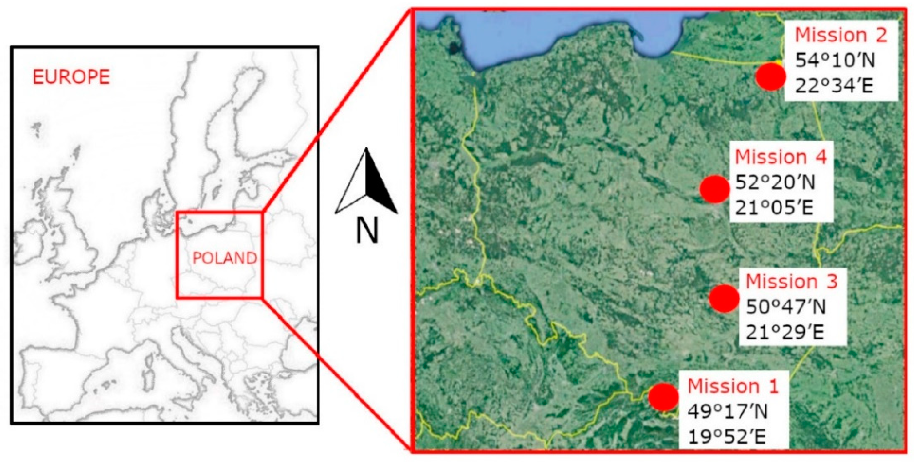
This study used datasets acquired from a low altitude by different unmanned platforms, under different weather and lighting conditions, and for areas with different topography and land cover (

Table 1. Summary of parameters of the photogrammetric missions.

	Mission 1	Mission 2	Mission 3	Mission 4
Site	mountainous	lowland, near lakes	upland	plain
Cloud cover	Max: 36%	Max: 90%	Max: 100%	Max: 16%
	Min: 4%	Min: 60%	Min: 40%	Min: 16%
Humidity	Max: 85%	Max: 90%	Max: 84%	Max: 81%
	Min: 45%	Min: 85%	Min: 77%	Min: 81%
Wind speed	Max: 12 m/s	Max: 20 m/s	Max: 17 m/s	Max: 9 m/s
	Min: 6 m/s	Min: 3 m/s	Min: 16 m/s	Min: 9 m/s
Sun azimuth	Max: 98.8°	Max: 232.1°	Max: 143.5°	Max: 148.8°
	Min: 259.7°	Min: 134.1°	Min: 117.4°	Min: 141.9°
Altitude	Max: 300 m	Max: 402 m	Max: 300 m	Max: 100 m
	Min: 21 m	Min: 24 m	Min: 75 m	Min: 50 m
Number of photos	291	168	243	1120
UAV	DJI Phantom 4 Pro	DJI Phantom 4 Pro	Parrot Sequoia	UX5

). Data were acquired in several different photogrammetric missions. Two missions were performed for flat terrain (Mission 1 in the lake district of northern Poland and Mission 4 in the lowland area in the centre of the country). The other two missions were performed in mountainous and upland areas (Figure 2).

A total of 1822 images were acquired in the missions. These images were characterised by different weather conditions (for Missions 1 and 2 the meteorological conditions were measured in situ, for 3 and 4 the data were obtained from [51]), different exposure parameters (set according to the external conditions), and the different nature of the terrain being imaged. Such a diversity of conditions made it possible to study series of real images of varying quality. Images acquired at approximately 90% humidity were hazy. Images acquired at high winds were blurred. The degree of cloud cover in turn affected image contrast and the amount of shadows, which had a significant impact on the quality of images from a wooded or urban area. In addition, sets of images were acquired at different times of the day and year, resulting in different azimuths of the sun. This is a factor that can affect the quality of the images, because the position of the sun determines how the area is illuminated. The influence of the sun position depends on the land cover and the case (different ceilings, platform tilt angles, different image coverage, etc.). Research focused on beach levelling considers image quality in terms of photogrammetry. They show that for noon flights the error can be almost double that for the early morning flights and it increases when forward overlap decreases [52]. Additionally, for the same fragments of terrain, series of photographs were taken from different altitudes and under different exposure conditions. This allowed us to take into account the relationship between UAV flight altitude and image quality as well as between selected exposure parameters and image quality. The main factors taken into account were exposure time, aperture size, and ISO, which affected the brightness and noise of the image.

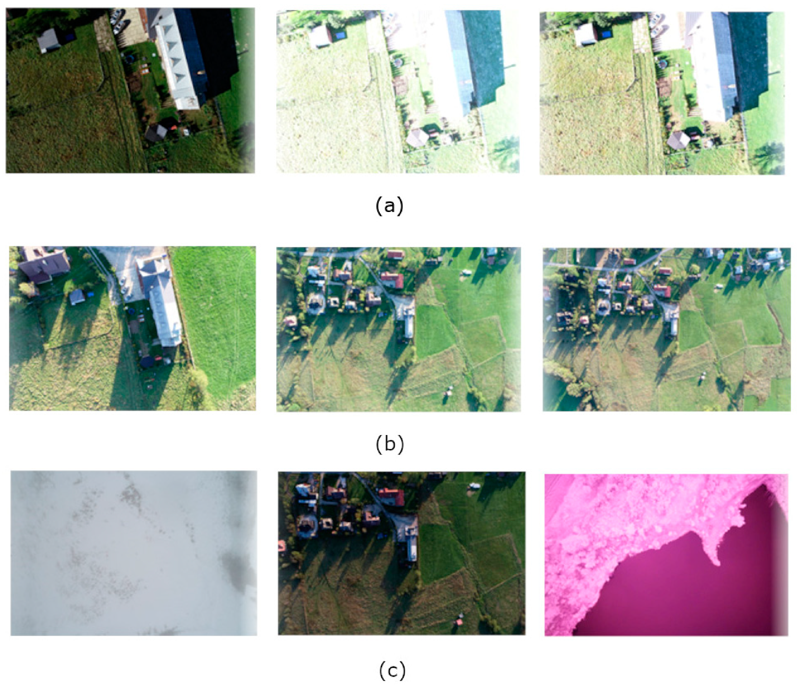
Each photogrammetric mission was carried out over an area of varying land cover. The database, therefore, included images of different types of land cover: fields, trees, lakes, snow, and buildings (Figure 3). The images were also captured with different sensors with different detector sensitivity ranges. The images used were from a UX5 fixed-wing airframe with a Sony Nex 5T camera imaging in the RGNIR (Red-Green-Near Infrared) range and from a 5N with a camera imaging in the RGB (Red-Green-Blue) range, and two rotary-wing platforms-the DJI Phantom 4 Pro with an RGB camera and a Parrot Sequoia recording separate images in the G, R, RedEdge, and NIR (Near Infrared) ranges.

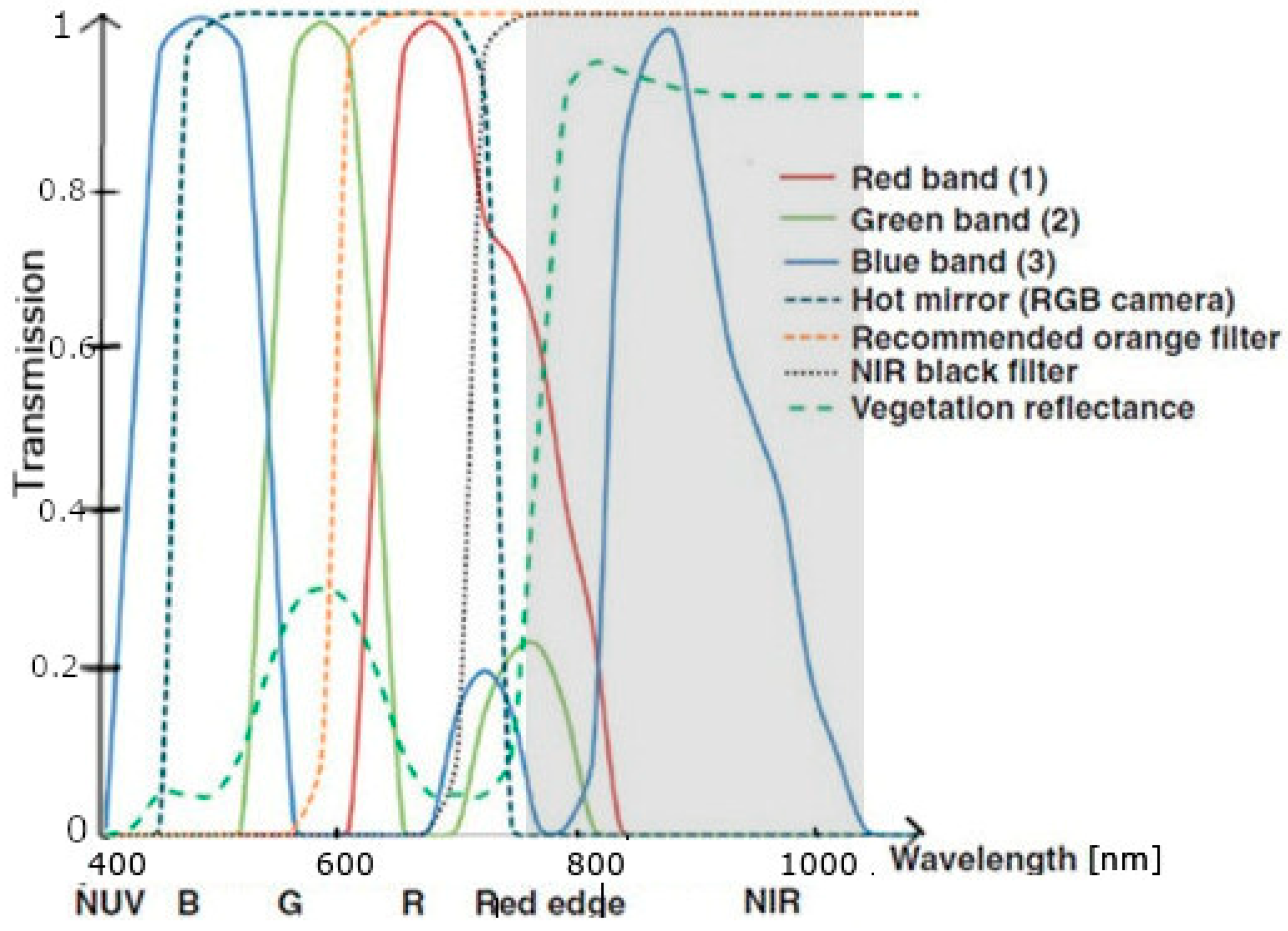
The UX5 is a fixed-wing UAV, mainly made of lightweight EPP foam and equipped with electric propulsion. The aircraft is launched using only a special mechanical launcher. The system can operate at wind speeds not exceeding 18 m/s and in conditions no worse than light rain. The Sony NEX-5T and Sony NEX-5N, which are mounted on this platform, are compact digital cameras equipped with 16.1-megapixel CMOS sensors (maximum image resolution is 4912 × 3264 pixels). The cameras are fitted with Voigtlander lenses with a fixed focal length of 15 mm and a maximum aperture of f/4.5. The Sony NEX-5N is a visible range imaging camera. The NEX-5T has been modified to allow shooting across the full sensitivity range of the sensor, so a filter was removed. The filter was located directly in front of the camera’s sensor, and it cut off the electromagnetic wave range above 690 nm. The maximum wavelength that can be recorded by the sensor is around 1050 nm. Images were acquired with a NIR-enabled camera with a black IR-only longpass filter, which cut on at 695 nm. Using this filter meant that the imagery contained NIR only, where the blue pixels (band 3) were again used to record nothing but pure NIR (roughly 800–1050 nm), while the red band (band 1) in the imagery obtained with this filter was, in fact, the red edge, roughly from 690 to 770 nm (Figure 4) [53].

The Parrot Sequoia is a sensor dedicated to remote sensing analyses studying vegetation and agricultural change. The system contains four detectors capturing images in the G (550 nm), R (660 nm), Red Edge (735 nm), and NIR (790 nm) ranges. It has an illumination sensor and a system that compensates for changing light conditions during image acquisition. The camera has a 16-megapixel CMOS sensor (maximum image resolution is 4608 × 3456 pixels) [54].

The DJI Phantom 4 is equipped with four electric motors and a navigation system, which uses the Global Positioning System/Global Navigation Satellite System (GPS/GLONASS) and an optical positioning system as well as two Inertial Measurement Unit (IMU) systems. A great advantage of the platform is its gimbal stabilized in three axes, on which a 1-inch 20-megapixel Complementary Metal-Oxide Semiconductor (CMOS) sensor with a mechanical shutter is installed. The camera installed on the platform acquires images in the RGB spectral range. The focal length of the lens is 24 mm (full-frame).

The whole set of acquired UAV images was divided into two parts: training data (70% of all data) and test data (30% of all data). Both training and test data varied in terms of acquisition conditions and image quality.

4. Methodology

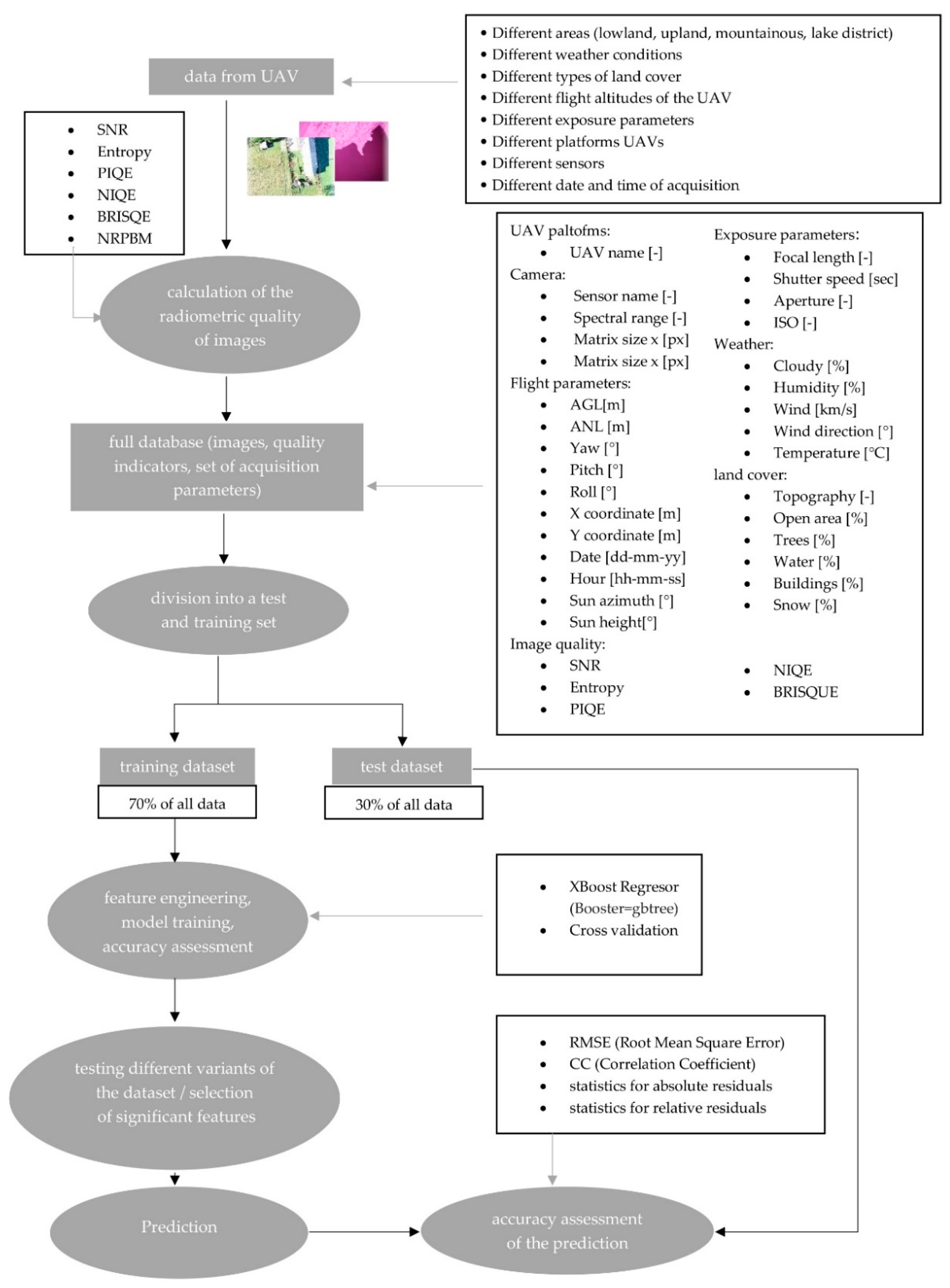
For each image among those acquired in the different low-altitude photogrammetric missions (described in the Data chapter), the radiometric quality was assessed. Several different indices were used for absolute evaluation of the results. The following were calculated: Entropy, SNR, NIQE, PIQE, BRISQUE, and NRPBM. The images, their metrics, and the set of indices formed a comprehensive database of information about image quality and acquisition conditions. This database was divided into two sets: a test dataset and a training dataset. Each object in the database had a set of features relating to sensor characteristics (sensor name and type, metric sensitisation range, focal length, ISO, aperture, and shutter speed), lighting conditions (date and time of acquisition, sun altitude and azimuth, and sensor tilt angles), weather conditions (cloud cover, fog, humidity, and air temperature), topography and land cover (terrain, variation in land cover, and nature of land cover, e.g., trees, meadows, buildings, and water). The diagram shows a general algorithm for image quality prediction based on a priori factors (Figure 5).

The XBoost Regressor model was used for image quality prediction. It is one of the most widely used models to solve classification and regression problems. Its effectiveness is much better than other simple models such as the Linear Regressor or the Decision Tree Regressor, because the XBoost Regressor mainly prevents overfitting of the model. XGBoost is a supervised learning technique. The approximation is performed by optimising specific loss functions and applying several regularisation techniques [55]. The problem under investigation required a regression-based solution. The Mean Square Error (MSE) was used as the loss function for optimization. This is the recommended function for target fields with a Gaussian distribution. MSE is calculated as the mean of the squared differences between the predicted and actual values. The result is always positive regardless of the sign of the predicted and actual value, and the ideal value is 0. Based on the MSE, the Root Mean Square Error (RMSE) was calculated and used later to evaluate the accuracy of the model. The Regularised Learning Objective was realised using the formula (Equation (1)) [56]

$$L^{\left(t\right)}\cong {{\displaystyle \sum }}_{i=1}^n[l(y_i, {\widehat{y}}^{\left(t-1\right)}+g_i{f}_t\left(x_i\right)+\frac{1}{2}{h}_i{f}_t^2\left(x_i\right)]+\Omega \left(f_t\right)$$

(1)

where l is the differentiable convex loss function that measures the difference between the prediction $\widehat{y_i}$ and the target $y_i$. Ω determines the complexity of the model. The lower the value of the loss function, the more accurate the predictions. Thus, obtaining better predictions will be solved by minimising the loss function. The minimisation is carried out by the function $f_t$. However, the functions $g_i$ and $h_i$ are first and second-order gradient statistics on the loss function. After removing the constant factors, Equation (1) takes the form (2) [56]

$${\tilde{L}}^{\left(t\right)}= {\sum }_{i=1}^n[g_i{f}_t\left(x_i\right)+ \frac{1}{2}{h}_i{f}_t^2\left(x_i\right)]+\Omega \left(f_t\right)$$

(2)

After developing the function $\Omega (f_t)$ and calculating the optimum weight $w_j$ for each leaf $j$ in the tree, the optimal values can be calculated using Equation (3) [56]

$${\tilde{L}}^{\left(t\right)}\left(q\right)= -\frac{1}{2}{\sum }_{j=1}^T\frac{{({\sum }_{i\in I_j}{g}_i)}^2}{{\sum }_{i\in I_j}{h}_i+\lambda }+\gamma T$$

(3)

where γ (gamma parameter) and λ (lambda parameter) are additional regularization parameters. Regularization aims to prevent overfitting of the model. In the case of overfitting or undertraining of the model, the values of the lambda and gamma parameters should be particularly modulated. Lambda is L2 regularization on the weights, which might help to reduce overfitting. It is responsible for the regulation of leaf weights and causes a smooth decrease in leaf weights, which forces strong limitation of leaf weights. Gamma is a pseudo-regularization parameter. The higher the gamma, the higher the regularization [56,57]. Regularization parameters depend on the number of features, the characteristics of the input data, and the complexity of the model. In this study, the following values were adopted: gamma equal to 0 and lambda raised to 2. The analysis of the accuracy of the predicted values did not indicate any undertraining or overfitting of the model.

This equation measures in practice how good a tree is. So, it enables choosing the best tree of all possible trees, but in practice, this is impossible because of the large amount of data and the large number of combinations (trees). The solution here is a certain optimization algorithm. It starts with a single leaf and iteratively adds branches to the tree. Each leaf is divided into two leaves (left and right) and the result of the division is (4) [56]

$$L_{split}=\frac{1}{2}[\frac{{({\sum }_{i\in I_L}{g}_i)}^2}{{\sum }_{i\in I_L}{h}_i+\lambda }+\frac{{({\sum }_{i\in I_R}{g}_i)}^2}{{\sum }_{i\in I_R}{h}_i+\lambda }- \frac{{({\sum }_{i\in I}{g}_i)}^2}{{\sum }_{i\in I}{h}_i+\lambda }] - \gamma$$

(4)

This equation allows us to assess the suitability of a branch. If the profit is less than $y_i$, it would be better not to add this branch. In this way, optimisation of tree building is ensured. By design, this prediction model builds the best tree among all possibilities, which is the reason for the effectiveness of the XBoost Regressor [56]. The booster was chosen as a tree model (called gbtree). This gives a better fit for nonlinear dependencies than the linear booster (gblinear) [58,59]. When considering a series of external factors affecting the quality of the images, it is expected that most of them will have a nonlinear effect.

The tree is built based on the dependencies that arise from the features of subsequent objects (low-altitude images). Therefore, the key stage is feature engineering, i.e., the selection and processing of features in such a way as to achieve the highest possible model quality. When selecting features for the prediction model, several variants were considered based on the different availability of preflight image data. The considered features were divided into several basic groups (imaging system parameters, meteorological conditions, terrain topography, and date and time of image acquisition). In each group, several analyses were performed to select the factors that had the greatest impact on image quality. Therefore, different variants of data influence on image quality were tested.

Case 1: UAV and camera parameters (camera and platform name, camera spectral sensitivity range, and array dimensions) and basic flight parameters (location, date and time, altitude above sea level (ASL), altitude above ground (AGL), azimuth, and sun altitude) are known. Case 2: only weather conditions are known (cloud cover, humidity, wind strength and direction, and temperature). Case 3: Case 1 plus topography and land cover (percentage of area covered by water, arable land, buildings, trees, and snow). Case 4–Case 1 plus image exposure parameters (focal length, aperture, ISO, and shutter speed). Case 5: Case 1 plus Case 2. Case 6: all features.

Immeasurable data (such as UAV platform names, sensor names, and topographies) were factorised. Each distinct feature value was assigned a unique numerical value. The spectral range was defined as an object type with values: RGB (colour images acquired with a camera acquiring in the visible range), RGNIR (colour images acquired with a camera with sensitivity from the Green to the near-infrared range), RED (monochrome images acquired with a sensor working in the Red range), GRE (monochrome images acquired with a sensor acquiring in the green range), REG (monochrome images acquired with a sensor recording in the Red Edge range), and NIR (monochrome images acquired with a sensor recording in the Near-Infrared range). In addition, for each image in each case, the image quality indices SNR, NIQE, PIQE, BRISQUE, NRPBM, and Entropy were calculated. These provided the basis for the model to identify the relationship between features and image quality.

In total, 1822 images with a set of features were used for the study, and six indicators of radiometric quality were counted for each of them. Seventy percent of the collected data was used to train the model, the remaining 30% was test data, which was used to assess the accuracy of the predictions. The prediction was based on a maximum of 26 features (case 6). Consequently, the number of observations significantly exceeded the number of features. The problem would be the number of features greater than the number of observations, as this would risk overloading the model.

Cross-validation was used for the machine learning model. Cross-validation allows the entire dataset to be used for both learning and model validation. It is used to determine the quality of the model while it is already being taught, in order to eliminate overfitting. Cross-validation consists of dividing the learning set into k equal subsets, of which k − 1 are used to train the model and 1 subset is used for model validation. Five hundred such divisions were made. Each of them contained a different data configuration. Consequently, the model was trained and validated 500 times. Each time it used different data for training and testing. Thus, in the end, all data were used for both training and validation. The root mean square error (RMSE), which was counted for each of the 500 configurations, was used to assess accuracy of the model. The model was evaluated for the accuracy of the determination of each of the SNR, NIQE, PIQE, BRISQUE, NRPBM, and Entropy. A statistical analysis of the RMSE values obtained is summarised in

Table 2. Statistics of RMSE values of determining SNR, NIQE, PIQE, BRISQUE, NRPBM, and Entropy indices in 6 variants of the a priori parameter set.

Quality Metric	Parameter	Case 1	Case 2	Case 3	Case 4	Case 5	Case 6
SNR	mean	0.58	0.56	0.81	1.23	0.51	0.45
	standard deviation	0.89	0.86	1.04	1.26	0.94	0.43
	maximum	10.16	9.77	10.94	11.64	11.05	5.65
	minimum	0.02	0.01	0.01	0.05	0.02	0.03
Entropy	mean	0.16	0.16	0.19	0.28	0.15	0.13
	standard deviation	0.25	0.27	0.28	0.34	0.27	0.18
	maximum	3.14	3.13	3.13	3.42	3.14	2.62
	minimum	0.01	0.01	0.01	0.02	0.00	0.01
NIQE	mean	0.16	0.15	0.2	0.3	0.14	0.14
	standard deviation	0.17	0.16	0.17	0.24	0.16	0.11
	maximum	1.76	1.74	1.74	1.59	1.73	0.91
	minimum	0.01	0.01	0.01	0.01	0.01	0.00
PIQE	mean	1.27	1.24	1.38	1.91	1.18	1.04
	standard deviation	2.58	2.54	2.52	2.5	2.74	1.63
	maximum	34.35	32.89	33.47	32	36.73	25.21
	minimum	0.08	0.04	0.05	0.1	0.05	0.03
BRISQUE	mean	2.48	2.42	2.89	4.62	2.35	2.22
	standard deviation	2.25	2.18	2.34	3.09	2.29	1.75
	maximum	24.58	24.63	24.58	26.82	24.67	24.12
	minimum	0.06	0.06	0.07	0.24	0.1	0.05

.

The highest model quality was obtained for Case 6 (after accounting for all possible factors). For each image quality assessment metric, the mean RMSE was the lowest. The standard deviations also reached the lowest values, which indicated a small spread of errors around the mean value. This in turn indicated that the model for Case 6 was the most accurate. Therefore, in the developed methodology a model was proposed, which takes into account both flight and sensor parameters, as well as weather conditions and topographic factors, terrain coverage, and exposure parameters. Nevertheless, only a series of basic parameters were used for the initial development of the model building concept. Factors that were not correlated with model quality were eliminated from the final version of the model. In order to diagnose them, a feature importance analysis was conducted for each image quality assessment metric (

Table 3. Importance of characteristics for Case 6.

Feature	SNR	Entropy	NIQE	PIQE	BRISQUE	NRPBM
AGL	0.0058	0.0880	0.7011	0.0143	0.0028	0.0030
ANL	0.0166	0.0075	0.0035	0.0100	0.0014	0.0002
building	0.8458	0.0030	0.0255	0.0036	0.0020	0.0008
cloudy	0.0005	0.0021	0.0071	0.0005	0.8899	0.0001
date	0.0006	0.0345	0.0008	0.0145	0.0037	0.0001
focal_length	0.0000	0.0000	0.0000	0.0000	0.0000	0.0000
hour	0.0004	0.0087	0.0038	0.0031	0.0020	0.0024
humidity	0.0000	0.0012	0.0000	0.1542	0.0009	0.0001
aperture	0.0006	0.0089	0.0181	0.0272	0.0017	0.0438
ISO	0.0019	0.0129	0.0013	0.0057	0.0026	0.0024
matrix_x	0.0000	0.0000	0.0000	0.0000	0.0000	0.0000
matrix_y	0.0000	0.0000	0.0000	0.0000	0.0000	0.0000
open_area	0.0011	0.0288	0.0227	0.0029	0.0248	0.0003
pitch	0.0003	0.0011	0.0005	0.0008	0.0004	0.0003
platforms	0.0000	0.0009	0.0008	0.0059	0.0001	0.9066
range	0.0020	0.0034	0.0029	0.0065	0.0087	0.0003
roll	0.0001	0.0020	0.0005	0.0005	0.0005	0.0001
sensor	0.0020	0.0423	0.0028	0.0280	0.0015	0.0016
shutter_speed	0.0140	0.1176	0.0245	0.0136	0.0157	0.0010
snow	0.0010	0.0436	0.0002	0.0131	0.0019	0.0168
sun_azimuth	0.0095	0.0225	0.0400	0.0422	0.0028	0.0007
sun_height	0.0025	0.0901	0.0175	0.0072	0.0066	0.0086
temperature	0.0000	0.0000	0.0002	0.0003	0.0004	0.0005
topography	0.0000	0.0000	0.0000	0.0000	0.0000	0.0000
tree	0.0084	0.0459	0.0019	0.0044	0.0018	0.0035
water	0.0658	0.0394	0.0763	0.0023	0.0149	0.0036
lift	0.0184	0.2148	0.0199	0.6210	0.0005	0.0000
wind_direction	0.0000	0.0000	0.0000	0.0000	0.0029	0.0000
Xcoord	0.0005	0.1295	0.0232	0.0127	0.0016	0.0014
yaw	0.0007	0.0034	0.0009	0.0020	0.0014	0.0005
Ycoord	0.0014	0.0478	0.0038	0.0035	0.0062	0.0013

). Factors marked in bold did not have any influence on the quality of the model and were not taken into account in learning the final version of the model.

Taking into account the above analysis of the importance of features, the tree prioritizes features in each category according to their importance (Figure 6). The average importance for all indicators for case 6 (with a full set of features) was taken into account.

Each subsequent feature in the category is less important for the quality of UAV imagery. The features separated by a dashed line have weights equal or very close to 0 for each indicator. Therefore, they can be considered as irrelevant from the point of view of the radiometric quality of the images.

In addition, new features created as a result of data engineering were included in the final version of Case 6. Combining some of the original features significantly improved the quality of the model. Therefore, additional features, which were functions of the primary features, were applied. According to research [7], the radiometric distortion of an image is influenced by the camera angles during image registration. However, when considering the yaw angle, it is the difference between the sun azimuth and the yaw angle that should be taken into account. It is this that largely causes the uneven illumination of the scene. Similarly, the quality of the model was positively affected by considering the difference between the wind direction and the azimuth of the unmanned platform.

5. Results

The results were analysed from two angles. Section 5.1 presents the feature importance analysis for the selected cases of the set of a priori known factors. In Section 5.2, the prediction accuracy of UAV image quality for each case is analysed. Case 6 (which produced the most accurate model) was enriched here with additional features arising from data engineering (wind_yaw_direction, the difference between wind direction and yaw angle and azimuth_difference, the difference between the azimuth of the sun and the UAV platform).

5.1. Feature Importance Analysis

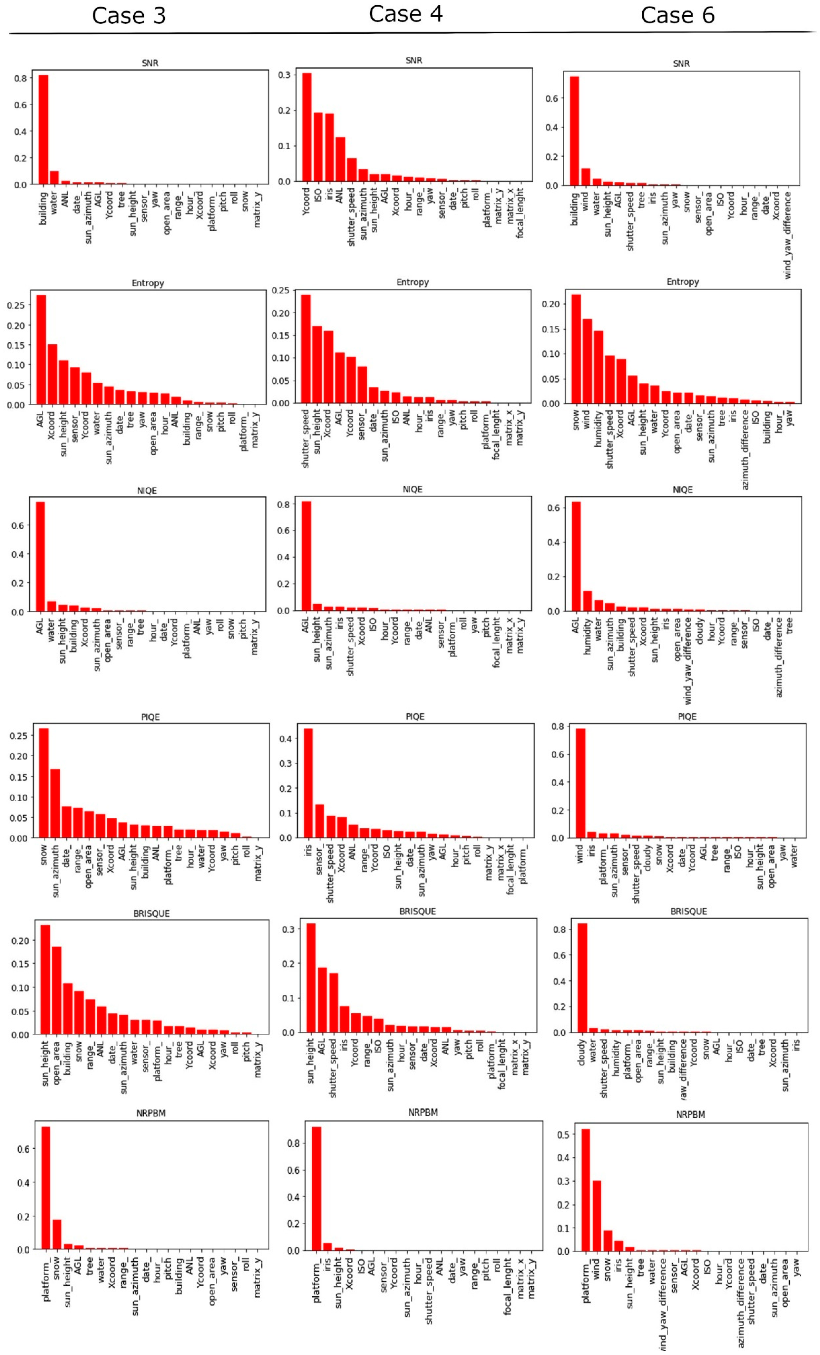
A feature importance analysis was conducted for each case. This analysis identified which features were most important in predicting a priori image quality. Figure 7 summarises the feature importance analysis for the three most characteristic variants (Case 3, Case 4, Case 6), assuming that these are the cases that can be encountered most often in practice. Case 3 assumes that before the flight we know the UAV and camera parameters as well as the topography and terrain coverage. Case 4 assumes that before the flight we know the UAV parameters, camera parameters, and photo exposure parameters. Case 6 assumes that before the flight a full set of information about the conditions of image acquisition is known.

The feature importance analysis for different metrics shows that different factors affect different aspects of image quality. It is not possible to determine a priori significant factors based on the values of only one metric. SNR and NIQE generally depend mainly on one factor. NIQE is highest for sharp images and lower for blurred and noisy images [60]. More than 70% of the influence on the NIQE value is due to AGL. Images acquired from high altitudes are more often blurred. In addition, they image a larger area and are more affected by uneven illumination, which can result in higher noise in less illuminated regions. In addition, at higher UAV flight altitudes, a greater influence of haze is observed [7], which also negatively affects the sharpness of the image. SNR depends mainly on the land cover. The greatest influence on its value is the presence of buildings and water in the images. Built-up areas, due to the large variety of imaged objects, are characterized by a large variance of pixel values. On the other hand, areas showing water have a very low variance, because the pixel values are then very close to each other. At the same time, with a higher variance, a higher number of false pixels, i.e., noise, can also be expected. Case 4 did not take land cover information into account and one main factor influencing SNR was not determined at that time. Case 4 shows that if the terrain coverage is not specified, the quality of the image will also be quite significantly affected by the exposure parameters and pixel location (coordinates). Pixel location is indirectly related to coverage. The ISO and the aperture size mainly influence the noise level of the image, as they determine the light sensitivity and the amount of light reaching the sensor.

Entropy, PIQE, and BRISQUE are dependent on many factors, but it is possible to select a certain group of factors that are important in predicting the values of these metrics. The most relevant features include AGL, terrain coverage (buildings, water, and snow), sun position, wind, shutter speed, aperture, humidity, and sensor type. Depending on the indicator, these factors affect the image quality to varying degrees. Wind and shutter speed have a key influence on image blur. In strong wind, the speed of the UAV can increase. Then, with too long an exposure time, the acquired images are blurred, so they are unreadable. In turn, high humidity increases haze, which also reduces image sharpness. NRPBM depends mainly on the type of platform and wind. These are two factors that significantly affect image blur. For UAVs equipped with a stabilizing gimbal, image blur is low. For platforms without stabilization or susceptible to wind (such as the UX5 airframe), the blurring of the image is higher.

To sum, out of the weather conditions, wind and humidity have the greatest influence on the quality of the imagery. Out of the exposure parameters, ISO, exposure time, and aperture are the most important. Also important is the information about ground cover.

The quality of UAV images is not affected by topography, as even in mountainous terrain the denivelations within one image are small. The influence of temperature has not been demonstrated either (in the range of 0–30 °C; the influence of lower and higher temperatures has not been studied, as it is not recommended to use a UAV in such conditions). The wind direction is of negligible importance and the size of the array does not influence the quality of the image in any way. For the above factors, the feature weights were 0 or very close to 0 for all indicators.

5.2. Accuracy of Prediction

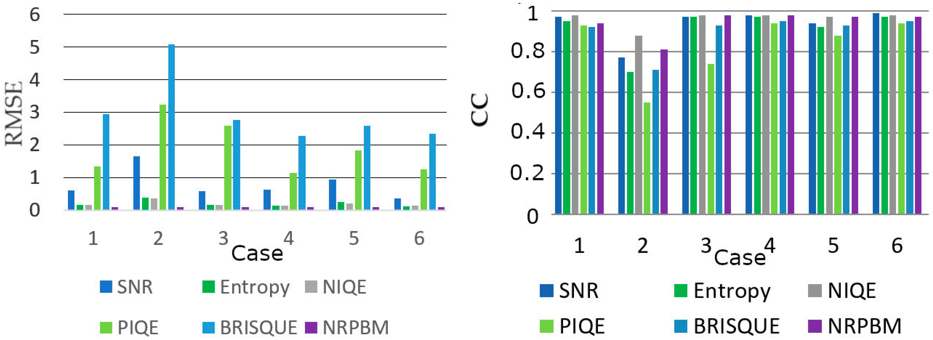
The present study aimed to investigate the possibility of predicting the quality of images a priori; therefore, a very important issue is the prediction accuracy. In order to evaluate the prediction accuracy, the actual image quality indices of the test set were compared with those predicted by the model. The RMSE error and CC correlation coefficient (Figure 8) were calculated for each case for each image quality indicator.

The lowest prediction accuracy was obtained for Case 2, where it was assumed that only weather conditions are known a priori. As can be seen from the analyses, such an assumption does not guarantee high prediction accuracy, so it is recommended to also take into account other factors influencing image quality. In other cases, RMSE values were lower, and the CC generally exceeded 0.9. The highest accuracy was achieved for Case 6, where the largest number of different factors were used (sensor parameters, flight parameters, weather, land cover, and exposure parameters). The correlation coefficient averaged 0.96. For entropy, NIQE, SNR, and NRPBM the RMSE values did not exceed 0.5. PIQE and BRISQUE, which have higher values, were determined with an accuracy of 1.2 and 2.3, respectively. The above shows that in order to achieve high accuracy of image quality prediction it is sufficient to know the parameters of the sensor, flight, and exposure. However, information on land cover and weather conditions may additionally increase the accuracy of this prediction.

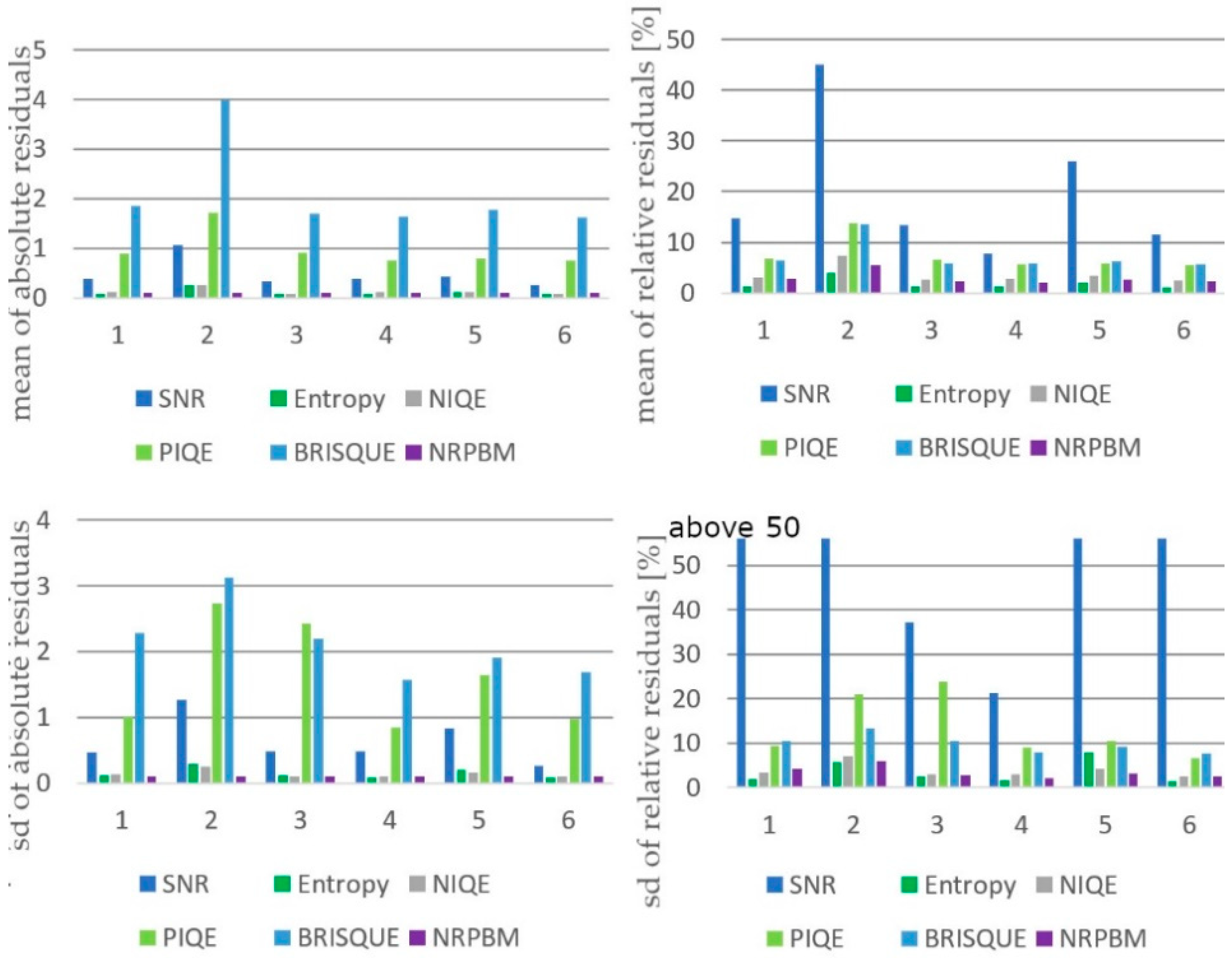
Additionally, the distribution of deviations between the actual and predicted values of the metrics was analysed. The graphs (Figure 9) show the standard deviations (SD) and mean values of the deviations. The results for relative and absolute deviations are summarised. Absolute deviations are the differences between the actual and predicted values. Relative deviations are the ratio of the absolute deviation to the actual value expressed as a percentage. In some cases, with very low actual metric values, this ratio was very large, shown in the graphs as a deviation above 50.

The mean value and standard deviation show the distribution of differences between the actual and predicted values. Higher absolute deviations occurred for PIQE and BRISQUE due to the higher values of these metrics. The relative deviations, on the other hand, allowed for a more reliable comparison of results between the different metrics. Considering the mean values of both types of deviations, the conclusions of the RMSE and CC analysis can be confirmed. The highest prediction accuracy was achieved for Cases 4 and 6, while the lowest was for Case 2. This is also confirmed by the standard deviations of the deviations. The lower the standard deviation, the smaller the spread of values around the mean. This in turn means that the results are more precise. The standard deviations of the deviations were the highest in Case 2 and the lowest in Case 6. Comparing the relative deviations, it can be seen that (except for SNR) both the mean and standard deviation were most similar for the different indicators in Case 6. This shows that this variant gives the most stable results and is the most reliable. Due to the relatively low SNR values, the relative deviations reach very high values here, which makes it impossible to interpret them properly. However, the absolute deviations show that the differences between the actual and predicted SNR values for Case 2 is 1.6 dB. In the remaining cases, they do not exceed 0.5 dB, which confirms the high prediction accuracy of this image quality indicator.

6. Discussion

The research aimed to develop a methodology for a priori prediction of UAV image quality. As part of the research, a methodology was designed, based on machine learning, to predict image quality based on a set of parameters known prior to flight. In addition, several variants of the parameters were investigated in order to determine the optimal requirements for the methodology. To date, most studies have focused on assessing image quality after a photogrammetric mission [3,34,35,61,62]. Low-quality images were often detected based on indicators and manually removed from the collection. In recent years there have been attempts to automate the selection of low-quality images [63]. However, these are still a posteriori analyses. This manuscript proposes a solution to estimate the quality of images before a flight, which often saves time, labour, and finances.

The study shows that the assessment of image quality cannot be based on a single indicator. Several metrics based on other relationships and focusing on other image features (noise, blur, sharpness, and information content) should always be considered. These conclusions are in line with other studies [3,41,64,65], where also image quality assessment was based on comparing results for several different metrics. The studies confirmed that conclusions based on only one indicator can be misleading and incomplete. SNR assesses the image in terms of noise but is not adequate to assess blur. Feature importance analysis has shown that different factors affect other aspects of image quality. It is not possible to establish a priori significant factors based on the values of only one metric. AGL has more than 70% influence on the NIQE value. SNR depends mainly on land cover. The largest influence on its value is the presence of buildings and water in the images, which is related to the large variance of the pixel values. NRPBM is mainly dependent on the type of platform and wind. On the other hand, Entropy, PIQE, and BRISQUE depend on many factors. The most relevant features include AGL, terrain coverage, sun position, wind, exposure speed, aperture, humidity, and sensor type. Research has therefore confirmed that it is not possible to evaluate and predict the quality of an image based on just one type of parameter. Both weather conditions and exposure or camera parameters should be taken into account. The results confirmed the findings of other studies that wind and shutter speed have a key influence on image blurring [63]. On the other hand, high humidity increases haze, which also reduces image sharpness [5,7]. In addition, the importance of lighting conditions and the camera-to-subject distance has been mentioned in other articles [66], which is also confirmed in this manuscript. One of the most important parameters affecting image quality turned out to be AGL, i.e., precisely the distance of the camera from the photographed area. Out of the exposure parameters, ISO, exposure time, and aperture have the strongest influence on image quality [8,10].

The proposed methodology gives the ability to predict image quality with high accuracy. The correlation coefficient exceeded 0.9 and for Case 6 (taking into account all factors known before the flight) was 0.96. The RMSE values for entropy, NIQE, SNR, and NRPBM did not exceed 0.5 (Case 6). PIQE and BRISQUE, which have higher values, were determined with an accuracy of 1.2 and 2.3, respectively. The study shows that knowledge of the sensor, flight, and exposure parameters is sufficient to achieve high accuracy in image quality prediction (Case 4). However, information about land cover and weather conditions can further improve the accuracy of this prediction.

The methodology was designed for data acquired from onboard UAVs. Similar prediction accuracy is expected for other images acquired from low altitude and close range. For other UAV platforms or other sensors, the model may require additional learning, but the results should not differ significantly (as these parameters were not crucial in assessing image quality). Due to the technical limitations of UAV platforms, images acquired at temperatures lower than 0 °C and higher than 30 °C, during rainfall, very strong winds, and from an altitude higher than 400 m were not included in the study. In case of the need to apply the model to data acquired in such non-standard conditions, the training base should be enriched with the above examples.

7. Conclusions

High radiometric image quality is essential for correct remote sensing analyses. In general, the quality of UAV images is evaluated after the flight and then a decision is made about the further value and use of the acquired data. This manuscript proposes an a priori image quality prediction methodology based on machine learning using the XBoost Regressor model and cross-validation. The model was learned on a rich database of real images acquired from UAVs under a variety of conditions. Different sensors, different UAV types, different exposure parameters, different flight parameters, different topography and land cover types, and different meteorological conditions were considered. The training and test base also included quality indicators for each image (SNR, Entropy, PIQE, NIQE, BRISQUE, and NRPBM) in order to train and test the model and image quality prediction accuracy, respectively. Different variants of preflight parameter knowledge were considered in the study. The proposed methodology offers the possibility of image quality prediction with high accuracy. The correlation coefficient generally exceeded 0.9, and for all factors known before the flight, it was 0.96. RMSE values for Entropy, NIQE, SNR, and NRPBM did not exceed 0.5, while PIQE and BRISQUE were determined with an accuracy of 1.2 and 2.3, respectively. The study shows that to achieve high accuracy of image quality prediction it is sufficient to know sensor, flight, and exposure parameters. However, information on land cover and weather conditions can further improve the accuracy of this prediction. The methodology was designed for data acquired from onboard UAVs. Similar prediction accuracy is expected for other images acquired from low altitudes. For other UAV platforms, other sensors or extremely non-standard acquisition conditions, the model may need to be refined.